Abstract

We derive the flow equations for the symmetry unbroken phase of a dilute 3-dimensional Bose gas. We point out that the flow equation for the interaction contains parts which are non-analytic at the origin of the frequency-momentum space. We examine the way this non-analyticity affects the fixed point of the system of the flow equations and shifts the value of the critical exponent for the correlation length closer to the experimental result in comparison with previous work where the non-analyticity was neglected. Finally, we emphasize the purely thermal nature of this non-analytic behaviour comparing our approach to a previous work where non-analyticity was studied in the context of renormalization at zero temperature.

1 Introduction

Thermal effective actions are in general non-local in coordinate space because the temperature-dependent Green functions contain parts which are non-analytic at the origin of the momentum-frequency space[1, 2]. In a theory with two interacting scalar fields, one integrates out one of them to find the effective action for the other. At finite temperature, provided the coupling is weak, one usually proceeds by applying perturbation theory, and then making an expansion in powers of frequency and momentum in order to obtain a local effective Lagrangian. It is this latter expansion which leads to results which are not uniquely defined but depend on the path on the frequency-momentum plane through which the origin is approached. For example, when the perturbation is truncated at the self-energy level, the self-energy is non-analytic at the origin. The reason is that the expansion is around a singularity [3].

This effect was noticed for the first time by Abrahams and Tsuneto in the 60’s, in the context of BCS theory, while they were studying time-dependent Ginzburg-Landau theory near zero temperature and near the critical temperature [4]. Later it became clear that it is the origin of Debye screening and of plasma oscillations in QED [5, 6]. These two different physical phenomena correspond to two different ways of approaching the origin of the momentum-frequency plane. The effects of the non-analyticity have also been studied in QED₃ [7] and in QCD [8, 9, 10, 11, 12, 13]. The non-analyticity is also present in the graviton self-energy [14, 15] and in higher-order graviton diagrams [16]. Even in the much simpler case of interacting scalars the non-analyticity of the self-energy persists [17, 18, 19, 20]. In the case of interacting scalars, an interesting remark is that, whenever the internal propagators in a loop have different masses, the self-energy is analytic at the origin [21]. The reason is that the singularity is not at the origin anymore, allowing thus a uniquely defined expansion around the origin.

This paper is based on the simple observation that an essential step of the renormalization group method (RG) applied to a theory with a self-interacting field, is to split the field in slow and fast components, and integrate out the fast field obtaining thus an effective action for the slow field [22, 23]. Therefore, according to the above discussion about thermal effective actions, when RG techniques are applied in the context of thermal field theory, we anticipate that effects originating in the non-analyticity will arise.

We choose to examine this aspect of RG in the context of a 3-dimensional homogeneous self-interacting bosonic gas with weak repulsive interactions and discuss its possible physical significance in this case. However our analysis and conclusions should hold whenever RG is used at finite temperature. This choice of system was motivated by the renewed interest in the Bose-Einstein condensation due to its recent experimental realization. For the interacting gas, the approach which is most often used is that of Bogoliubov. However, this is just a mean-field type method and, in principle, one can improve upon it by using more sophisticated techniques. One possibility near the critical region is the renormalization group [24, 25, 26, 27].

In the case of the homogeneous gas, there is an extra, more important reason for looking for alternatives to the Bogoliubov approach. In the critical region, the Bogoliubov theory simply does not work because there are fluctuations around the mean-field that cannot be treated perturbatively. This happens because, as the temperature approaches the critical temperature $T_{c}$, the thermal cloud density develops an infrared singularity and thus diverges as the momentum tends to zero [28, 29].

In section 2, we introduce the basics of the BEC formalism above the critical region. We then apply Wilsonian renormalization and derive the flow equations for the parameters of the Lagrangian. We point out the non-analytic structure of the RG correction to the interaction term (vertex) and follow this non-analyticity as it propagates to the flow equation for the interaction.

In section 3, we calculate the non-trivial fixed pont of the system of the flow equations and find the critical exponent for the correlation length. We examine the way the non-analyticity affects the fixed point. We note that taking the non-analyticity into account shifts the value of the critical exponent closer to the experimental result.

In section 4, we compare our work with [30] where the issue of non-analyticity in the context of renormalization is also discussed. We point out that the conclusions of [30] hold only at $T=0$ whereas the non-analytic behaviour which we are investigating in this paper is purely thermal and vanishes at zero temperature, thus being completely independent of the non-analyticity discussed in [30].

In section 5, we present our conclusions.

2 Non-analyticity in the uncondensed phase

When the two-body collisions between bosons are taken to be low-momentum or s-wave, the path integral representation of the partition function of the homogeneous interacting Bose-gas is given by

$$Z(\mu,\beta,V,g)\equiv{\rm Tr}e^{-\beta(\hat{H}-\mu\hat{N})}=\int\delta[\phi,\phi^{*}]e^{-S[\phi,\phi^{*}]}$$ (1)

with the action

$$S[\phi,\phi^{*}]=\frac{1}{\hbar}\int_{0}^{\hbar\beta}d\tau\int_{V}d^{D}{\bf x}\left[\phi^{*}(\tau,{\bf x})[\hbar\frac{\partial}{\partial\tau}-\frac{\hbar^{2}}{2m}\nabla^{2}-\mu]\phi(\tau,{\bf x})+\frac{1}{2}g|\phi(\tau,{\bf x})|^{4}\right].$$ (2)

In the low-momentum approximation the interparticle interaction can be described by the zero-momentum component of the Fourier transform of the two-body interaction potential. Thus, within this approximation, a repulsive, short-range potential can be characterized by a positive interaction strength $g$. In three spatial dimensions this interaction strength is related to the positive scattering length $a$ of the interparticle interaction by the familiar relation $g=4\pi\hbar^{2}a/m$. The chemical potential is denoted by $\mu$. The case $\mu<0$ holds for $T>T_{c}$ and corresponds to the uncondensed phase whereas $\mu>0$ describes the condensate which is formed when $T<T_{c}$ [31]. In this paper we will deal only with the uncondensed phase. Starting from (2) we can derive the renormalization group equations for $g$ and $\mu$. This set of coupled differential equations can then be used for the study of universal as well as non-universal properties of the gas [24, 25, 26, 27]. In the following we will set $\hbar=1$.

In order to implement the first step of the RG procedure (Kadanoff transformation), we split the field $\phi(x)$ into a long-wavelength component $\phi_{<}(x)$ and into a short-wavelength component $\delta\phi_{>}(x)$. The short-wavelength field involves Fourier components which are contained only in an infinitesimally thin shell in momentum space of thickness $\Lambda(1-dl)\leq|{\bf p}|\leq\Lambda$ near the cutoff $\Lambda$, whereas the long-wavelength field has all its Fourier components in the sphere whose center is at the origin of the momentum space and its radius is $\Lambda(1-dl)$. We impose no cutoff on the frequency and apply the Wilsonian technique of consecutive infinitesimal shell integration only to the momentum and not to the frequency [32].

We denote the volume of the shell by $\delta V_{{\bf p}}$, the volume of the sphere by $V_{{\bf p}}$. The coordinate space volume is denoted by $V$. For simplicity we will be referring to $\phi_{<}(x)$ as the lower or slow field and to $\delta\phi_{>}(x)$ as the upper or fast field. Whenever more compact notation is required we will be making use of the following:

$$x=(\tau,{\bf x}),\hskip 28.45274ptp=(p_{0}^{n},{\bf p})\hskip 28.45274pt{\rm with}\hskip 28.45274ptp_{0}^{n}=2\pi n/\beta,$$

$$\int dx=\int_{0}^{\beta}d\tau\int_{V}d^{3}{\bf x},\hskip 28.45274pt\int dp=\frac{1}{\beta}\;\sum_{n=-\infty}^{\infty}\int\frac{d^{3}{\bf p}}{(2\pi)^{3}}.$$

We integrate out the upper field and are left with an effective action for the lower field

$$S_{\rm eff}[\phi_{<},\phi_{<}^{*}]=S[\phi_{<},\phi_{<}^{*}]+\frac{1}{2}{\rm Tr}{\rm Ln}[1-\hat{G}^{>}\hat{\Sigma}].$$ (3)

For details on the derivation of this result and the approximations involved see [23]. The ${\rm Tr}$ denotes the trace in both the functional and the internal space of $\hat{G}^{>}\hat{\Sigma}$ whereas the ${\rm tr}$ denotes the trace only in the internal space (see below). The hat denotes that the corresponding quantity is a Schwinger-Fock operator [33],

$$\hat{G}^{>}(\hat{p})=\left(\begin{array}[]{cc}B(\hat{p})&0\\ 0&B^{*}(\hat{p})\end{array}\right)$$

and

$$\hat{\Sigma}(\hat{x})=\frac{g}{2}\left(\begin{array}[]{cc}4\phi^{*}_{<}(\hat{x})\phi_{<}(\hat{x})&2\phi_{<}(\hat{x})\phi_{<}(\hat{x})\\ 2\phi_{<}^{*}(\hat{x})\phi_{<}^{*}(\hat{x})&4\phi^{*}_{<}(\hat{x})\phi_{<}(\hat{x})\end{array}\right)$$

with

$$B(\hat{p})=B(\hat{p}_{0},\hat{{\bf p}})=\frac{1}{i\hat{p}_{0}+E(\hat{{\bf p}})},\hskip 56.9055ptE(\hat{{\bf p}})=\frac{\hat{{\bf p}}^{2}}{2m}-\mu.$$ (4)

Note that the expression for ${\hat{\Sigma}}$ contains the coupling $g$. This enables us to perform a perturbative expansion over $g$ in (3) in order to calculate it explicitly. We truncate this expansion to second order in $g$

$${\rm Tr}{\rm Ln}[1-\hat{G}^{>}\hat{\Sigma}]\approx{\rm Tr}[-\hat{G}^{>}\hat{\Sigma}-\frac{1}{2}(\hat{G}^{>}\hat{\Sigma})^{2}].$$

The first trace is:

$${\rm Tr}[\hat{G}^{>}\hat{\Sigma}] =\int dx~{}\int dp~{}{\rm tr}[G^{>}(p)\Sigma(x)]$$ (5)

$$=\int dx~{}|\phi_{<}(x)|^{2}2g\int_{\delta V_{{\bf p}}}\frac{d^{3}{\bf p}}{(2\pi)^{3}}[1+2N[E({\bf p})]]$$

where $N[E({\bf p})]=[e^{\beta[E({\bf p})]}-1]^{-1}$ is the Bose-Einstein distribution. We note that the first trace is quadratic in the modulus of the lower field and can therefore be interpreted as a correction to the chemical potential

$$d\mu=-g\int_{\delta V_{{\bf p}}}\frac{d^{3}{\bf p}}{(2\pi)^{3}}[1+2N[E({\bf p})]].$$ (6)

The second trace is:

$${\rm Tr}[\hat{G}^{>}\hat{\Sigma}\hat{G}^{>}\hat{\Sigma}]=\int dp\int dk\int dx\int dy\;e^{i(p-k)(y-x)}\;{\rm tr}[G^{>}(p)\Sigma(x)G^{>}(k)\Sigma(y)]=$$

$$\int dp\int dk\int dx\int dy\;e^{i(p-k)(y-x)}\;\frac{g^{2}}{4}$$

$$\left[16\;B(p)\;B(k)\;\phi_{<}^{*}(x)\;\phi_{<}(x)\;\phi_{<}^{*}(y)\phi_{<}(y)\;+4\;B(p)\;B^{*}(k)\;\phi_{<}(x)\;\phi_{<}(x)\;\phi_{<}^{*}(y)\;\phi_{<}^{*}(y)\;+\right.$$

$$\left.4\;B^{*}(p)\;B(k)\;\phi_{<}^{*}(x)\;\phi_{<}^{*}(x)\;\phi_{<}(y)\;\phi_{<}(y)\;+16\;B^{*}(p)\;B^{*}(k)\;\phi_{<}^{*}(x)\;\phi_{<}(x)\;\phi_{<}^{*}(y)\;\phi_{<}(y)\;\right].$$

In order to simplify the above expression we change variables as follows:

1. In the second and fourth terms in the square brackets, $p\rightarrow-p$ and $k\rightarrow-k$.

2. In the second term, $x\rightarrow y$ and $y\rightarrow x$.

The second trace now becomes:

$${\rm Tr}[\hat{G}^{>}\hat{\Sigma}\hat{G}^{>}\hat{\Sigma}]=\int dp\int dk\int dx\int dy\;\frac{g^{2}}{4}$$

$$\left\{\left[e^{i(p-k)(y-x)}+e^{i(k-p)(y-x)}\right]\;B(p)\;B(k)\;16\;\phi_{<}^{*}(x)\;\phi_{<}(x)\;\phi_{<}^{*}(y)\;\phi_{<}(y)\;\right.$$

$$\left.+2e^{i(p-k)(y-x)}\;B^{*}(p)\;B(k)\;4\;\phi_{<}^{*}(x)\;\phi_{<}^{*}(x)\;\phi_{<}(y)\;\phi_{<}(y)\right\}.$$ (8)

Changing variables again, $k\rightarrow q=k-p$, yields:

$${\rm Tr}[\hat{G}^{>}\hat{\Sigma}\hat{G}^{>}\hat{\Sigma}]=\int dq\int dx\int dy\;\frac{g^{2}}{4}$$

$$\left\{2\;e^{-iq(y-x)}\;J_{1}(q)\;4\;\phi_{<}^{*}(x)\;\phi_{<}^{*}(x)\;\phi_{<}(y)\;\phi_{<}(y)\;\right.$$

$$\left.+\left[e^{-iq(y-x)}+e^{iq(y-x)}\right]\;J_{2}(q)\;16\;\phi_{<}^{*}(x)\;\phi_{<}(x)\;\phi_{<}^{*}(y)\;\phi_{<}(y)\;\right\}$$ (9)

where

$$J_{1}(q_{0}^{m},{\bf q})=\int dp\;B^{*}(p)\;B(p+q)\hskip 28.45274pt{\rm and}\hskip 28.45274ptJ_{2}(q_{0}^{m},{\bf q})=\int dp\;B(p)\;B(p+q).$$ (10)

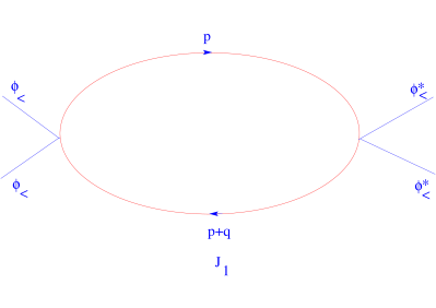
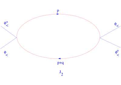
Figure 1: The two contributions of the RG correction to the interaction g, $J_{1}$ and $J_{2}$; $p$ is the frequency-momentum of the upper field (the momentum ${\bf p}$ is integrated over the infinitesimal shell around the cutoff), $q$ is the frequency-momentum of the lower field.

We note that ${\bf p}$ is the momentum of the upper field (integrated over the infinitesimal shell around the cutoff) whereas ${\bf q}$ is the momentum of the lower field, Fig.1.

It is essential in the RG procedure, and in particular in the Kadanoff transformation, to recast the effective action obtained after integrating out the upper field in the form of the original action (2). The first trace is in a form that can be interpreted as a correction to the chemical potential. This is not the case however for the second trace; there are quartic products of fields but, unlike the four-field coupling term in the original action (2), these are non-local in coordinate space, thus not allowing the effective action to be recast in the form of the original action. In other words, though we start from an action containing interactions which are local in coordinate space, the RG procedure generates more general, non-local interactions.

This is a well-known feature of RG, namely to generate extra terms that do not appear in the original action and have a more general form in comparison to what we started with [22, 34, 35]. Provided that these extra terms are not relevant they can, in most cases, for the purpose of calculating universal properties, be discarded.

In our case we can Taylor expand $\phi_{<}(y)$ around $\phi_{<}(x)$. If we truncate this expansion at leading order, $\phi_{<}(y)\approx\phi_{<}(x)$, we remain within the family of local interactions we started with. This procedure is usually called derivative expansion and is physically relevant only when the lower field is slowly varying both in space and in time.

Wilsonian renormalization is compatible with the derivative expansion. The reason is that in Wilsonian renormalization we are interested in constructing an effective action for the slow field. This compatibility can also be seen from a more technical point of view; the derivative expansion of the lower field is equivalent to an expansion of $J_{1}$ and $J_{2}$ in powers of $q_{0}$ and ${\bf q}$ (this is easily seen from (9) doing integration by parts). This means that truncating the derivative expansion at higher than the leading order would give momentum and frequency dependent corrections to the interaction. However such terms are known to be irrelevant (see for example [34], page 128) and can therefore be omitted.

The second trace becomes:

$${\rm Tr}[\hat{G}^{>}\hat{\Sigma}\hat{G}^{>}\hat{\Sigma}]=\int dx\;\frac{g^{2}}{4}$$

$$\left\{\lim_{q\rightarrow 0}[2e^{iqx}J_{1}(q)]\ 4\phi_{<}^{*}(x)\phi_{<}^{*}(x)\phi_{<}(x)\phi_{<}(x)+\lim_{q\rightarrow 0}[(e^{iqx}+e^{-iqx})J_{2}(q)]\ 16\phi_{<}^{*}(x)\phi_{<}(x)\phi^{*}_{<}(x)\phi_{<}(x)\right\}$$

which is a local expression that can be interpreted as a correction to the coupling term of the original action

$$dg=-g^{2}\left\{\lim_{(q_{0}^{m},|{\bf q}|)\rightarrow(0,0)}[J_{1}(q_{0}^{m},{\bf q})]+4\lim_{(q_{0}^{m},|{\bf q}|)\rightarrow(0,0)}[J_{2}(q_{0}^{m},{\bf q})]\right\}.$$ (12)

It is at this point that the non-analyticity enters our discussion. Because we are at finite temperature, the integrals over frequencies in $J_{1}$ and $J_{2}$, $I_{1}$ and $I_{2}$ respectively, become sums which can be easily calculated when we turn them into integrals on the complex plane through Poisson summation

$$J_{1}(q_{0}^{m},{\bf q})=\int_{\delta V_{{\bf p}}}\frac{d^{3}{\bf p}}{(2\pi)^{3}}\;I_{1}(q_{0}^{m},{\bf q},{\bf p})\hskip 28.45274pt{\rm and}\hskip 28.45274ptJ_{2}(q_{0}^{m},{\bf q})=\int_{\delta V_{{\bf p}}}\frac{d^{3}{\bf p}}{(2\pi)^{3}}\;I_{2}(q_{0}^{m},{\bf q},{\bf p})$$ (13)

where

$$I_{1}(q_{0}^{m},{\bf q},{\bf p})=\frac{1}{\beta}\sum_{n=-\infty}^{\infty}B^{*}(p_{0}^{n},{\bf p})B(p_{0}^{n}+q_{0}^{m},{\bf p+q}))=\frac{1+N[E({\bf p})]+N[E({\bf p}+{\bf q})]}{E({\bf p}+{\bf q})+E({\bf p})-iq_{0}^{m}},$$ (14)

$$I_{2}(q_{0}^{m},{\bf q},{\bf p})=\frac{1}{\beta}\sum_{n=-\infty}^{\infty}B(p_{0}^{n},{\bf p})B(p_{0}^{n}+q_{0}^{m},{\bf p}+{\bf q}))=\frac{N[E({\bf p})]-N[E({\bf p}+{\bf q})]}{E({\bf p}+{\bf q})-E({\bf p})+iq_{0}^{m}}.$$ (15)

We have set $\exp{i\beta q_{0}^{m}}=1$ because $q_{0}^{m}=2\pi m/\beta$. In the following, we will suppress the superscript of $q_{0}^{m}$ for simplicity.

The first sum, $I_{1}$, is non-vanishing at $T=0$ and is known as the regular term. The second sum, $I_{2}$, is purely thermal and is usually called Landau term in the context of thermal field theory [2]. We observe that the successive limits of $J_{1}(q_{0},{\bf q})$ coincide, i.e.

$$\lim_{q_{0}\rightarrow 0}\lim_{|{\bf q}|\rightarrow 0}J_{1}(q_{0},{\bf q})=\int_{\delta V_{{\bf p}}}\frac{d^{3}{\bf p}}{(2\pi)^{3}}\frac{1}{2E({\bf p})}\left[1+2N[E({\bf p})]\right]=\lim_{|{\bf q}|\rightarrow 0}\lim_{q_{0}\rightarrow 0}J_{1}(q_{0},{\bf q})$$ (16)

whereas the successive limits of $J_{2}(q_{0},{\bf q})$ do not

$$\lim_{q_{0}\rightarrow 0}\lim_{|{\bf q}|\rightarrow 0}J_{2}(q_{0},{\bf q})=0\neq\lim_{|{\bf q}|\rightarrow 0}\lim_{q_{0}\rightarrow 0}J_{2}(q_{0},{\bf q})=\int_{\delta V_{{\bf p}}}\frac{d^{3}{\bf p}}{(2\pi)^{3}}\beta e^{\beta E({\bf p})}N^{2}[E({\bf p})].$$ (17)

The reason these two limits do not commute is that $J_{2}$ has a singularity at the origin of the momentum-frequency space [3]. Of course, in the evaluation of the above limits, we interchanged the limits with both the integration over the momentum $|{\bf p}|$ and with the angular integration over $\theta$, so our conclusion is not entirely reliable so far. In principle, one should perform the integrations over $|{\bf p}|$ and $\theta$ first, and then take the limit. Unfortunately, in our case, the integration over $|{\bf p}|$ cannot be done analytically. However, we can perform the angular integration over $\theta$ analytically before evaluating the limits, provided that we split the integral as follows

$$J_{2}(q_{0},{\bf q})=\int_{\delta V_{{\bf p}}}\frac{d^{3}{\bf p}}{(2\pi)^{3}}\frac{N[E({\bf p})]}{E({\bf p}+{\bf q})-E({\bf p})+iq_{0}}-\int_{\delta V_{{\bf p}}}\frac{d^{3}{\bf p}}{(2\pi)^{3}}\frac{N[E({\bf p}+{\bf q})]}{E({\bf p}+{\bf q})-E({\bf p})+iq_{0}}$$ (18)

and perform the change of variables ${\bf p}\rightarrow-{\bf p}-{\bf q}$ in the second term, eliminating thus the dependence of the Bose-Einstein distribution on the angle $\theta$ and making the angular integration possible. This procedure yields the result

$$J_{2}(q_{0},{\bf q})=\int_{\delta V_{{\bf p}}}\frac{d^{3}{\bf p}}{(2\pi)^{3}}\left[\frac{1}{E({\bf p}+{\bf q})-E({\bf p})+iq_{0}}+\frac{1}{E({\bf p}+{\bf q})-E({\bf p})-iq_{0}}\right]N[E({\bf p})].$$ (19)

It is crucial to note that this change of variables is not permissible in case we interchange the limit $\lim_{|{\bf q}|\rightarrow 0}\lim_{q_{0}\rightarrow 0}$ with the integrations, because this causes both the terms in (18) to diverge. These two divergencies canceled each other before the change of variables ${\bf p}\rightarrow-{\bf p}-{\bf q}$ [7]. Keeping this remark in mind we now perform the angular integration and find

$$J_{2}(q_{0},{\bf q})=\frac{m}{4\pi^{2}}\int_{\Lambda-d\Lambda}^{\Lambda}d|{\bf p}|\frac{|{\bf p}|N[E({\bf p})]}{|{\bf q}|}\ln{\left[\frac{(E_{+}-E({\bf p}))^{2}+q_{0}^{2}}{(E_{-}-E({\bf p}))^{2}+q_{0}^{2}}\right]}$$ (20)

where $E_{+}=E(|{\bf p}|+|{\bf q}|)$ and $E_{-}=E(|{\bf p}|-|{\bf q}|)$. Instead of just taking the two successive limits in $J_{2}$ as we did before, which in the momentum-frequency plane corresponds to approaching the origin in the direction of the one or the other axis, we could approach the origin through any other curve, for example in the direction of any straight line $q_{0}=a|{\bf q}|$. Here, of course, we should not forget that the frequency is discrete whereas the momentum is continuous. However, for the purpose of better illuminating the structure of $J_{2}$ around the origin, we shall make the approximation that the frequency is continuous so that $q_{0}=a|{\bf q}|$ can hold for any real $a$. Applying this parameterization to (20) and then taking the limit $|{\bf q}|\rightarrow 0$ yields

$$\lim_{|{\bf q}|\rightarrow 0}J_{2}(a|{\bf q}|,|{\bf q}|)=\frac{m}{4\pi^{2}}\int_{\Lambda-d\Lambda}^{\Lambda}d|{\bf p}|N[E({\bf p})]\frac{2|{\bf p}|^{2}}{|{\bf p}|^{2}+m^{2}a^{2}}$$ (21)

which reproduces the first limit of (17) for $a\rightarrow\infty$. This result was derived from (20) and therefore is also not valid when the limit $a\rightarrow 0$ is interchanged with the integration over $|{\bf p}|$. However, if we do an integration by parts, we find

$$\lim_{|{\bf q}|\rightarrow 0}J_{2}(a|{\bf q}|,|{\bf q}|)=\frac{m}{2\pi^{2}}\left[N[E({\bf p})]\frac{|{\bf p}|^{3}}{|{\bf p}|^{2}+m^{2}a^{2}}\right]_{\Lambda-d\Lambda}^{\Lambda}$$

$$+\frac{1}{2\pi^{2}}\int_{\Lambda-d\Lambda}^{\Lambda}d|{\bf p}||{\bf p}|^{2}\left[\frac{|{\bf p}|^{2}}{|{\bf p}|^{2}+m^{2}a^{2}}\beta e^{\beta E({\bf p})}N^{2}[E({\bf p})]-\frac{2m^{3}a^{2}}{[|{\bf p}|^{2}+m^{2}a^{2}]^{2}}N[E({\bf p})]\right].$$ (22)

We note that the surface term vanishes, as it is evaluated at the cutoff. This result not only reproduces the first limit of (17) for $a\rightarrow\infty$ but also agrees with the second limit of (17) for $a\rightarrow 0$. If we perform the angular integration and apply the same parameterization to $J_{1}$, at the limit $|{\bf q}|\to 0$, $J_{1}$ is independent of $a$ and given by (16). Expressions (16) and (22) are to be substituted in the correction for the coupling constant (12).

Before we proceed to the second step of the RG formalism, we parameterize the momentum according to $|{\bf p}(l)|=\Lambda e^{-l}$. The purpose this change of variables serves is simply to make the flow equations more elegant.

So far, the flow equation for the chemical potential is:

$$\frac{d\mu}{dl}=-g\frac{\Lambda^{3}e^{-3l}}{2\pi^{2}}[1+2N[\epsilon_{\Lambda}e^{-2l}-\mu]]$$ (23)

and the flow equation for the coupling is:

$$\frac{dg}{dl}=-g^{2}\left\{\frac{\Lambda^{3}e^{-3l}}{2\pi^{2}}\frac{1}{2[\epsilon_{\Lambda}e^{-2l}-\mu]}[1+2N[\epsilon_{\Lambda}e^{-2l}-\mu]]+\right.$$

$$\left.4\frac{\Lambda^{3}e^{-3l}}{2\pi^{2}}\left[\frac{\Lambda^{2}e^{-2l}}{\Lambda^{2}e^{-2l}+m^{2}a^{2}}\beta N[\epsilon_{\Lambda}e^{-2l}-\mu][1+N[\epsilon_{\Lambda}e^{-2l}-\mu]]-\frac{2m^{3}a^{2}}{[\Lambda^{2}e^{-2l}+m^{2}a^{2}]^{2}}N[\epsilon_{\Lambda}e^{-2l}-\mu]\right]\right\}$$

(24)

where $\epsilon_{\Lambda}=\Lambda^{2}/2m$.

At this point we apply the second step of the RG procedure, namely the trivial rescaling, whose purpose is to bring the effective action in the form of the original one. There are two stages, first, we rescale the momentum according to $|{\bf q}|\rightarrow|{\bf q}(l)|=|{\bf q}|e^{l}$ in order to re-establish the original cutoff $\Lambda$. Then we require that the effective Lagrangian has the same form as the original Lagrangian. This induces the trivial rescaling of the parameters of the effective Lagrangian.

$$V \to V(l)=V~{}e^{-3l},$$

$$\beta \to \beta(l)=\beta~{}e^{-2l},$$

$$\phi \to \phi(l)=\phi~{}e^{3l/2},$$

$$\mu \to \mu(l)=(\mu+\Delta\mu)~{}e^{2l},$$

$$g \to g(l)=(g+\Delta g)~{}e^{-l}.$$ (25)

The trivial rescaling of $\beta$ implies that the frequency is rescaled as $q_{0}\rightarrow q_{0}(l)e^{-2l}$ and therefore

$$a=q_{0}/|{\bf q}|\rightarrow a(l)\;e^{-l}.$$ (26)

Recasting (23) and (24) in terms of rescaled variables yields the flow equations for the corresponding running quantities

$$\frac{d\mu(l)}{dl}=2\mu(l)-g(l)\frac{\Lambda^{3}}{2\pi^{2}}[1+2N_{l}]$$ (27)

and

$$\frac{dg(l)}{dl}=-g(l)-g^{2}(l)\frac{\Lambda^{3}}{2\pi^{2}}\left\{\frac{1+2N_{l}}{2[\epsilon_{\Lambda}-\mu(l)]}+4\left[\frac{\Lambda^{2}}{\Lambda^{2}+m^{2}a^{2}(l)}\beta(l)N_{l}[1+N_{l}]-\frac{2m^{3}a^{2}(l)}{[\Lambda^{2}+m^{2}a^{2}(l)]^{2}}N_{l}\right]\right\}$$ (28)

where $N_{l}=[e^{\beta(l)[\epsilon_{\Lambda}-\mu(l)]}-1]^{-1}$ is the Bose-Einstein distribution in terms of the rescaled variables.

3 Fixed Point

It is important to investigate whether the path-dependence of the flow equation for the coupling has any consequences on quantities of physical interest.

We look at a universal property, the critical exponent for the correlation length. This is calculated from the coupled system of (27) and (28). In fact, in order to have an autonomous system, we should also take into account the flow equation for the inverse temperature,

$$\frac{d\beta(l)}{dl}=-2\beta(l)$$ (29)

which is just a differential expression of the trivial scaling of $\beta$ (25). We observe that, although $\beta$ appears in the equations for $\mu$ and $g$, these do not couple back to the equation for $\beta$. We also note that the fixed point for $\beta$ is zero, $\beta_{*}=0$. The fact that $\beta_{*}=0$ complicates things because $\beta(l)$ appears in the flow equations not only explicitly but also through $N_{l}$. This means that, when we evaluate the fixed point for the system of the flow equations, the right-hand side of (27) and (28) will diverge, because $N_{l}$ diverges for $\beta_{*}=0$. This problem is circumvented when we define a scaled running chemical potential $M(l)$ and a scaled running coupling constant $\tilde{G}(l)$ such that the set of equations for these new parameters decouples from the equation for $\beta$;

$$M(l)=\beta_{\Lambda}\mu(l)\hskip 28.45274pt{\rm and}\hskip 28.45274pt\tilde{G}(l)=\Lambda^{3}\beta_{\Lambda}g(l)/b(l)$$ (30)

where $\beta_{\Lambda}=m/\Lambda^{2}$, $\epsilon_{>}=1/2$ and $b(l)=\beta(l)/\beta_{\Lambda}$ is the scaled inverse temperature. In terms of these new, dimensionless parameters

$$\frac{dM(l)}{dl}=2M(l)-\frac{1}{2\pi^{2}}\tilde{G}(l)b(l)[1+2N_{l}],$$

$$\frac{d\tilde{G}(l)}{dl}=\tilde{G}(l)-\frac{1}{2\pi^{2}}\tilde{G}^{2}(l)b(l)\left\{\frac{1+2N_{l}}{2[\epsilon_{>}-M(l)]}+4\left[\frac{\Lambda^{2}}{\Lambda^{2}+m^{2}a^{2}(l)}b(l)N_{l}[1+N_{l}]-\frac{1}{\beta_{\Lambda}}\frac{2m^{3}a^{2}(l)}{[\Lambda^{2}+m^{2}a^{2}(l)]^{2}}N_{l}\right]\right\},$$

$$\frac{db(l)}{dl}=-2b(l).$$ (31)

In the neighbourhood of the fixed point, the rescaled temperature is high and the approximation $N_{l}\approx[\beta(l)[\epsilon_{\Lambda}-\mu(l)]]^{-1}=[b(l)[\epsilon_{>}-M(l)]]^{-1}$ holds [24]. This yields the equations

$$\frac{dM(l)}{dl}=2M(l)-\frac{1}{2\pi^{2}}\tilde{G}(l)\;b(l)\;[1+2\frac{1}{b(l)[\epsilon_{>}-M(l)]}],$$

$$\frac{d\tilde{G}(l)}{dl}=\tilde{G}(l)-\frac{1}{2\pi^{2}}\tilde{G}^{2}(l)\left\{\frac{b(l)}{2[\epsilon_{>}-M(l)]}+\frac{1}{[\epsilon_{>}-M(l)]^{2}}+4\frac{\Lambda^{2}}{\Lambda^{2}+m^{2}a^{2}(l)}\;\frac{b(l)}{\epsilon_{>}-M(l)}\right.$$

$$\hskip 34.14322pt\left.+4\frac{\Lambda^{2}}{\Lambda^{2}+m^{2}a^{2}(l)}\;\frac{1}{[\epsilon_{>}-M(l)]^{2}}-4\frac{2\Lambda^{2}m^{2}a^{2}(l)}{[\Lambda^{2}+m^{2}a^{2}(l)]^{2}}\;\frac{1}{\epsilon_{>}-M(l)}\right\},$$

$$\frac{db(l)}{dl}=-2b(l).$$ (32)

At the fixed point $(M_{*},\tilde{G}_{*},b_{*}=0)$ the left hand side of (32) is zero by definition. The form of the right hand side depends subtly on whether $a$ is zero or not as we will see. Near the fixed point, the second term is dominant in the square brackets of the flow equation for the chemical potential in (32),

$$\frac{dM(l)}{dl}=2M(l)-\frac{1}{\pi^{2}}\tilde{G}(l)\frac{1}{\epsilon_{>}-M(l)}.$$ (33)

For $a=0$, we recall (26), which means that $a(l)=0$ for any $l$. Consequently, the equation for the coupling reduces to

$$\frac{d\tilde{G}(l)}{dl}=\tilde{G}(l)-\frac{1}{2\pi^{2}}\tilde{G}^{2}(l)\left\{\frac{b(l)}{2[\epsilon_{>}-M(l)]}+\frac{1}{[\epsilon_{>}-M(l)]^{2}}+4\frac{b(l)}{\epsilon_{>}-M(l)}+4\frac{1}{[\epsilon_{>}-M(l)]^{2}}\right\}.$$ (34)

Recalling the trivial scaling of $b$ (25), we see that the second and fourth terms in the curly brackets above are dominant near the fixed point,

$$\frac{d\tilde{G}(l)}{dl}=\tilde{G}(l)-\frac{1}{2\pi^{2}}\tilde{G}^{2}(l)\frac{5}{[\epsilon_{>}-M(l)]^{2}}$$ (35)

and calculate the non-trivial fixed point

$$(M_{*},\tilde{G}_{*},b_{*})=(\frac{1}{12},\frac{5}{4}\frac{\pi^{2}}{18},0).$$

We linearize the system of (32) around the fixed point and find the largest eigenvalue $\lambda_{+}=1.878$. Therefore the critical exponent for the correlation length is $\nu=0.532$, which agrees with the one found in [24].

For $a\neq 0$, according to the trivial scaling of $a$ (26), $a_{*}=\infty$ and therefore the first and the third terms in the curly brackets of (32) vanish near the fixed point, as in the case of $a=0$. From the remaining terms the fifth vanishes and, significantly, the fourth is also vanishing near the fixed point, leaving as dominant contribution only the second term. Consequently the flow equation for the coupling reduces to

$$\frac{d\tilde{G}(l)}{dl}=\tilde{G}(l)-\frac{1}{2\pi^{2}}\tilde{G}^{2}(l)\frac{1}{[\epsilon_{>}-M(l)]^{2}}$$ (36)

and the non-trivial fixed point is

$$(M_{*},\tilde{G}_{*},b_{*})=(\frac{1}{4},\frac{\pi^{2}}{8},0).$$

Linearizing around the fixed point we find that $\lambda_{+}=1.561$ and therefore $\nu=0.640$. It is interesting to note that we could have found the same fixed point and critical exponent directly from (32), had we set $a=\infty$ and therefore $a(l)=\infty$ for any $l$.

This situation is similar to what happens, for example, in the case of thermal QED for the photon propagator. Because the photon self-energy is non-analytic at the origin, different ways of approaching the origin lead to different dispersion relations and give rise to different types of excitations [1, 2]. For short wavelengths, the dispersion relation is $q_{0}^{2}={\bf q}^{2}+m_{P}^{2}$, where $m_{P}^{2}=(e^{2}/2)(T^{2}/3+\mu^{2}/\pi^{2})$ is the thermal mass for the transverse photons whereas the longitudinal photons do not propagate. However, for long wavelengths, the transverse photons have the dispersion $q_{0}^{2}=\omega_{P}^{2}+\frac{6}{5}{\bf q}^{2}$ and the longitudinal photons have the dispersion $q_{0}^{2}=\omega_{P}^{2}+\frac{3}{5}{\bf q}^{2}$, where $\omega_{P}^{2}=\frac{2}{3}m_{P}^{2}$ is the plasma frequency at order $e^{2}$. The phenomenon which we are describing here is of the same mathematical nature, the difference being that it is occurring not in the propagator but in the vertex between four bosons. To be more precise it is the vertex graph corresponding to $J_{2}$, Fig.1, that exhibits the same singular behaviour as the photon self-energy in QED.

Comparing the two critical exponents derived above with the known experimental value $\nu=0.670$ [36], it becomes clear that the second procedure gives an improved estimate. In fact, our estimate is better even than the value $\nu=0.613$ calculated in [24] with the inclusion of the marginal three-body scattering term in the action.

4 Flow equations and non-analyticity at zero and finite temperature

Non-analyticity in the context of RG has been discussed before by Shankar in [30]. In this work, the author gives a detailed overview of the RG approach to interacting, non-relativistic fermions in one, two and three dimensions and in certain instances (pages 161, 166, 170, 178) refers to the non-analyticity (or lack thereof) which appears in the one-loop RG corrections to the quartic interaction among fermions. This is highly reminiscent of the case we are studying, the essential difference being that we are dealing with bosons instead of fermions. This would render the main point of this paper - the study of a non-analyticity in the flow equation for the interaction - rather trivial and expected by extending [30] to bosons.

This is not the case however, the non-analyticity we are studying is of completely different nature from the one studied in [30]. The RG calculations in [30] are at $T=0$ whereas ours at $T\neq 0$ and the non-analyticity we are referring to is essentially thermal and vanishes at $T=0$. To further clarify this point, let us consider the ”zero sound” (ZS) graph which is studied in Eq.(315), page 161 of [30].

4.1 Zero Temperature Non-Analyticity

4.1.1 Zero Sound Integral

In the zero-sound calculation of [30], the following integral appears:

$$S_{1}[\Omega,q]=\int_{-\Lambda}^{\Lambda}\frac{dk}{2\pi}\int_{-\infty}^{\infty}\frac{d\omega}{2\pi}\ \frac{1}{[i\omega-k][i(\omega+\Omega)-k-q]}$$ (37)

where $\Omega$, $q$ are the external frequency and momentum and $\omega$, $k$ are the internal frequency and momentum respectively. The external momentum is constrained by the same cutoff as the internal momentum, $-\Lambda\leq q\leq\Lambda.$

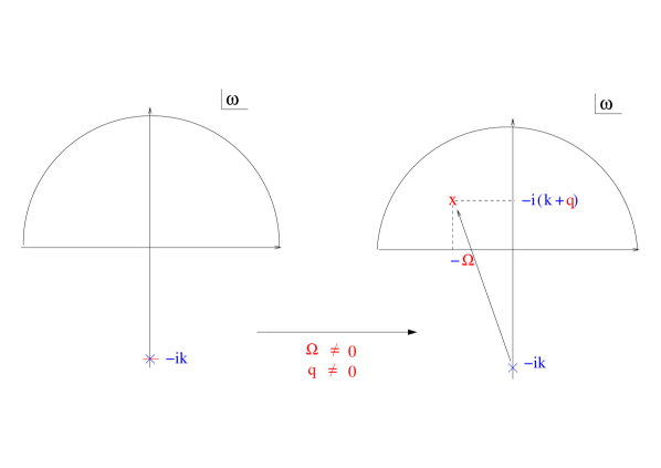
Figure 2: The integrand of the $\omega$-integration has one double pole and the integral is zero. Any non-zero external momentum splits the double pole into two single poles. There is always a range of $k$ for which the two single poles reside in different half-planes and consequently the integral is non-vanishing.

We focus on the integral over $\omega$. When the external momentum and frequency are zero, the integrand has a double pole and therefore $S_{1}[0,0]=0$, Fig.2.

For non-zero external frequency and momentum, the integrand has two single poles. Let us assume that $k>0$. If $k+q>0$, both poles are in the lower half-plane and closing the contour from above yields $S_{1}[\Omega,q]=0$. However, if $k+q<0$, the two single poles are in different half-planes and closing the contour either from above or below yields

$$S_{1}[\Omega,q]=\int_{-\Lambda}^{\Lambda}\frac{dk}{2\pi}\frac{i}{\Omega+iq}.$$

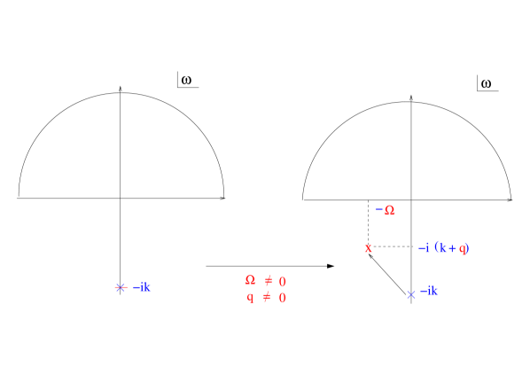
Figure 3: The integrand of the $\omega$-integration has one double pole and the integral is zero. The introduction of non-zero external momentum splits the double pole into two single poles. However, because the $k$-integration is over the infinitesimal shell near the cutoff and the external momentum $q$ takes value below the infinitesimal shell, the two single poles are always on the same half-plane and the integral remains zero.

Assuming $k<0$ we can argue the same way, so, only when $k$ and $k+q$ have different signs, the $\omega$-integral is non-zero, Fig.3.

Because of the $k$-integration, there is always a range of $k$ values for which $k$ and $k+q$ have different signs. Therefore any non-zero $q$ results in a non-vanishing

$$S_{1}[\Omega,q]=\int_{-\Lambda}^{\Lambda}\frac{dk}{2\pi}\frac{i}{\Omega+iq}[\theta(k)-\theta(k+q)]$$

which depends sensitively on how the limit $\{\Omega,q\}\to\{0,0\}$ is taken [30],

$$\lim_{\Omega\to 0}\lim_{q\to 0}S_{1}[\Omega,q]=0\neq\lim_{q\to 0}\lim_{\Omega\to 0}S_{1}[\Omega,q]=-1.$$

4.1.2 Renormalization Integral

In the RG calculation of [30], a one-loop correction to the interaction is of the form:

$$S_{2}[\Omega,q]=\left[\int_{-\Lambda}^{-\Lambda+d\Lambda}+\int_{\Lambda-d\Lambda}^{\Lambda}\right]\frac{dk}{2\pi}\int_{-\infty}^{\infty}\frac{d\omega}{2\pi}\ \frac{1}{[i\omega-k][i(\omega+\Omega)-k-q]}.$$ (38)

As before, for zero external frequency and momentum, $S_{2}[0,0]=0$.

For non-zero external frequency and momentum, we note that $S_{2}$ differs from $S_{1}$ only in the range of integration of the momenta, $k\in[-\Lambda,-\Lambda+d\Lambda]\cup[\Lambda-d\Lambda,\Lambda]$ and $q\in[-\Lambda+d\Lambda,\Lambda-d\Lambda]$. This means that $|k|>|q|$ and consequently $k,k+q$ have always the same sign throughout the integration over $k$. Therefore $S_{2}[\Omega,q]=0$ which has no dependence on how the limits of the external frequency and momentum are taken [30].

The conclusion is that, when performing RG calculations, non-analyticities at the origin of external frequency and momentum space vanish, even when they are present in the corresponding zero-sound calculations.

4.2 Thermal Non-Analyticity

4.2.1 Zero Sound Integral

Now consider what happens at $T\neq 0$. In zero-sound calculations one has to perform the integral

$$S_{1}^{\rm{T}}[\Omega_{m},q]=\int_{-\Lambda}^{\Lambda}\frac{dk}{2\pi}\frac{1}{\beta}\sum_{n=-\infty}^{n=\infty}\ \frac{1}{[i\omega_{n}-k][i(\omega_{n}+\Omega_{m})-k-q]}$$ (39)

where $\omega_{n}=(2n+1)\pi/\beta$, $\Omega_{m}=(2m+1)\pi/\beta$ are the discretized internal and external frequencies respectively.

When the external frequency and momentum are zero, we find

$$S_{1}^{\rm{T}}[0,0]=-\int_{-\Lambda}^{\Lambda}\frac{dk}{2\pi}\frac{\beta}{4}\cosh^{-2}[\frac{k\beta}{2}]\stackrel{{\scriptstyle\rm{T}\to 0}}{{\longrightarrow}}-1.$$ (40)

For non-zero external frequency and momentum, we obtain

$$S_{1}^{\rm{T}}[\Omega_{m},q]=\int_{-\Lambda}^{\Lambda}\frac{dk}{2\pi}\frac{i}{\Omega_{m}+iq}\frac{1}{2}\left\{\tanh{[\frac{k\beta}{2}]}-\tanh{[\frac{(k+q)\beta}{2}]}\right\}$$ (41)

which gives the correct zero temperature limit $S_{1}^{\rm{T}\to 0}[\Omega_{m},q]=S_{1}[\Omega,q]$. At $T\neq 0$,

$$\lim_{\Omega_{m}\to 0}\lim_{q\to 0}S_{1}^{\rm{T}}[\Omega_{m},q]=0\stackrel{{\scriptstyle\rm{T}\to 0}}{{\longrightarrow}}0,$$ (42)

$$\lim_{q\to 0}\lim_{\Omega_{m}\to 0}S_{1}^{\rm{T}}[\Omega_{m},q]=-\int_{-\Lambda}^{\Lambda}\frac{dk}{2\pi}\frac{\beta}{4}\cosh^{-2}[\frac{k\beta}{2}]\stackrel{{\scriptstyle\rm{T}\to 0}}{{\longrightarrow}}-1$$ (43)

and therefore the non-analyticity of the zero-temperature zero-sound calculation persists at finite temperatures, Fig.4.

4.2.2 Renormalization Integral

As at $T=0$, the integral appearing in RG calculations, differs from $S_{1}^{\rm{T}}$ only in the range over which the internal and external momentum are integrated.

When the external frequency and momentum are zero, we find

$$S_{2}^{\rm{T}}[0,0]=-\left[\int_{-\Lambda}^{-\Lambda+d\Lambda}+\int_{\Lambda-d\Lambda}^{\Lambda}\right]\frac{dk}{2\pi}\frac{\beta}{4}\cosh^{-2}[\frac{k\beta}{2}]\stackrel{{\scriptstyle\rm{T}\to 0}}{{\longrightarrow}}0.$$ (44)

For non-zero external frequency and momentum, we obtain

$$S_{2}^{\rm{T}}[\Omega_{m},q]=\left[\int_{-\Lambda}^{-\Lambda+d\Lambda}+\int_{\Lambda-d\Lambda}^{\Lambda}\right]\frac{dk}{2\pi}\frac{1}{\beta}\sum_{n=-\infty}^{\infty}\ \frac{1}{[i\omega_{n}-k][i(\omega_{n}+\Omega_{m})-k-q]}.$$ (45)

Poisson summation yields, Fig.4,

$$S_{2}^{\rm{T}}[\Omega_{m},q]=\left[\int_{-\Lambda}^{-\Lambda+d\Lambda}+\int_{\Lambda-d\Lambda}^{\Lambda}\right]\frac{dk}{2\pi}\frac{i}{\Omega_{m}+iq}\frac{1}{2}\left\{\tanh{[\frac{k\beta}{2}]}-\tanh{[\frac{(k+q)\beta}{2}]}\right\}$$ (46)

which gives the correct zero-temperature limit

$$S_{2}^{\rm{T}\to 0}[\Omega_{m},q]=0.$$

However, unlike the zero temperature renormalization integral, the finite temperature renormalization integral is non-analytic, because

$$\lim_{\Omega_{m}\to 0}\lim_{q\to 0}S_{2}^{\rm{T}}[\Omega_{m},q]=0\stackrel{{\scriptstyle\rm{T}\to 0}}{{\longrightarrow}}0,$$ (47)

$$\lim_{q\to 0}\lim_{\Omega_{m}\to 0}S_{2}^{\rm{T}}[\Omega_{m},q]=-\left[\int_{-\Lambda}^{-\Lambda+d\Lambda}+\int_{\Lambda-d\Lambda}^{\Lambda}\right]\frac{dk}{2\pi}\frac{\beta}{4}\cosh^{-2}[\frac{k\beta}{2}]\stackrel{{\scriptstyle\rm{T}\to 0}}{{\longrightarrow}}0.$$ (48)

Therefore, at finite temperature, the non-analyticity of the zero-sound one-loop graph persists but there is also an extra, purely thermal non-analyticity appearing in the finite temperature renormalization one-loop graph.

The zero temperature non-analyticities are due to the splitting of a double pole into two single poles residing in different half-planes. The finite temperature non-analyticities are due only to the splitting of a double pole and appear even if the resulting two single poles reside in the same half-plane. Therefore it is only natural that extra non-analyticities appear at finite temperature in addition to those existing at zero-temperature.

5 Conclusions

We have investigated thermal non-analyticities at the origin of the momentum-frequency space in the context of Wilsonian renormalization. We have shown that taking them into account leads to an improved estimate for the critical exponent of the correlation length, when approaching the critical region from the symmetry unbroken phase. It is well-known that the $\epsilon$-expansion gives values closer to the experiment than ours, however one should remember that the $\epsilon$-expansion is asymptotic [36]. It is therefore crucial to find safer ways of calculating the critical exponent, such as the improved momentum-shell method which was used here.

When approaching the critical region from the symmetry-broken phase there is an excellent estimate $\nu=0.685$ [24]. It may be possible to improve this value by taking into account the non-analyticity as we did for the approach from the symmetry unbroken phase. Work on this issue is currently under progress.

Finally, we have pointed out that when one applies Wilsonian renormalization at finite temperature, one may encounter non-analytic behaviour which is different in nature from the non-analyticity (or lack thereof) discussed in [30].

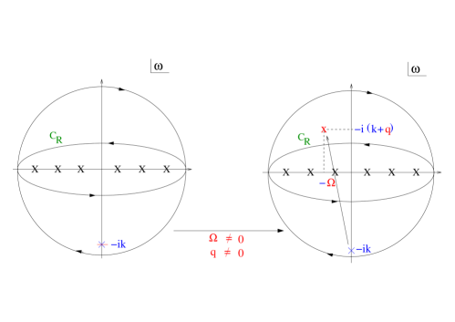
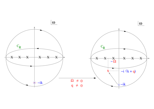
Figure 4: The integrand of the $\omega$-integration has one double pole. The introduction of non-zero external momentum splits the double pole into two single poles and the integral is non-vanishing regardless of whether the two single poles are on different half-planes or not.

References

- [1] J. I. Kapusta, Finite-Temperature Field Theory (Cambridge University Press, England, 1989).
- [2] M. LeBellac, Thermal Field Theory (Cambridge University Press, England, 1996).
- [3] H. A. Weldon, Phys.Rev. D28, 2007 (1983).
- [4] E. Abrahams and T. Tsuneto, Phys.Rev. 152, 416 (1966).
- [5] G. Baym, J. P. Blaizot, and B. Svetitsky, Phys.Rev. D46, 4043 (1992).
- [6] E. Petitgirard, Z.Phys. C54, 673 (1992).
- [7] I. J. R. Aitchison and J. A. Zuk, Ann.Phys. 242, 77 (1995).
- [8] O. K. Kalashnikov and V. V. Klimov, Sov. J. Nucl. Phys. 31, 699 (1980).
- [9] H. A. Weldon, Phys.Rev. D26, 1394 (1982).
- [10] V. V. Klimov, Sov. J. Nucl. Phys. 33, 934 (1981).
- [11] H. A. Weldon, Phys.Rev. D26, 2789 (1982).
- [12] E. Braaten and R. D. Pisarski, Nucl.Phys. B337, 569 (1990).
- [13] J. Frenkel and J. C. Taylor, Nucl. Phys. B334, 199 (1990).
- [14] A. Rebhan, Nucl. Phys. B368, 479 (1992).
- [15] A. Rebhan, Nucl. Phys. B351, 706 (1991).
- [16] J. Frenkel and J. C. Taylor, Z.Phys. C49, 515 (1991).
- [17] A. Das and M. Hott, Phys.Rev. D50, 6655 (1994).
- [18] Y. Fujimoto and H. Yamada, Z. Phys. C37, 265 (1988).
- [19] H. A. Weldon, Phys.Rev. D47, 594 (1993).
- [20] T. S. Evans, Z. Phys. C36, 153 (1987).
- [21] P. Arnold, S. Vokos, P. Bedaque, and A. Das, Phys.Rev. D47, 4698 (1993).
- [22] K. G. Wilson and J. Kogut, Phys.Rep. 12, 75 (1974).
- [23] R. J. Creswick and F. W. Wiegel, Phys.Rev. A28, 1579 (1983).
- [24] H. T. C. Stoof and M. Bijlsma, Phys.Rev. A54, 5085 (1996).
- [25] G. Alber, Phys.Rev. A63, 023613 (2001).
- [26] G. Alber and G. Metikas, Appl.Phys. B73, 773 (2001).
- [27] J. O. Andersen and M. Strickland, Phys.Rev. A60, 1442 (1999).
- [28] M. Rasolt, M. J. Stephen, M. Fischer, and P. Weichman, Phys.Rev.Lett 53, 798 (1984).
- [29] K. Burnett, in Bose-Einstein Condensation in Atomic Gases, Societá Italiana di Fisica, edited by M. Inguscio, S. Stringari, and C. E. Wieman (IOS, Varenna, 1998), Vol. CXL.
- [30] R. Shankar, Rev.Mod.Phys. 66, 129 (1994).
- [31] A. L. Fetter and J. D. Walecka, Quantum Theory of Many-Particle Systems (McGraw-Hill, N.Y., 1971).
- [32] J. A. Hertz, Phys.Rev B14, 1165 (1976).
- [33] J. Schwinger, Phys.Rev. 82, 664 (1951).
- [34] M. E. Fisher, in Lecture Notes in Physics (Springer, Heidelberg, 1983), Vol. 186, p. 1.
- [35] J. Cardy, Scaling and Renormalization in Statistical Physics (Cambridge University Press, England, 1996).
- [36] J. Zinn-Justin, Quantum Field Theory and Critical Phenomena (Oxford University Press, England, 1989).