Translational Symmetry Breaking in the Superconducting State of the Cuprates:
Analysis of the Quasiparticle Density of States

Abstract

Motivated by recent STM experiments on $\rm{Bi_{2}Sr_{2}CaCu_{2}O_{8+\delta}}$ [1, 2, 3, 4, 5], we study the effects of weak translational symmetry breaking on the quasiparticle spectrum of a $d$-wave superconductor. We develop a general formalism to discuss periodic charge order, as well as quasiparticle scattering off localized defects. We argue that the STM experiments in $\rm{Bi_{2}Sr_{2}CaCu_{2}O_{8+\delta}}$ cannot be explained using a simple charge density wave order parameter, but are consistent with the presence of a periodic modulation in the electron hopping or pairing amplitude. We review the effects of randomness and pinning of the charge order and compare it to the impurity scattering of quasiparticles. We also discuss implications of weak translational symmetry breaking for ARPES experiments.

]

I Introduction

Puzzling properties of the high-$T_{c}$ cuprates have often been attributed to the existence of competing instabilities, and proximity (or even coexistence) of several ordered states. Possible instabilities that have been discussed in this context include charge density wave (CDW) order, non-two-sublattice spin density wave (SDW) order [6, 7, 8, 9], spin Peierls order [10], and orbital magnetism [11, 12]. Neutron scattering experiments on $\rm{La_{1.6-\it{x}}Nd_{0.4}Sr_{\it{x}}CuO_{4}}$  [13], $\rm{La_{\it{x}}Sr_{1-\it{x}}CuO_{4}}$  [14, 15], and $\rm{La_{2}CuO_{4+\it{x}}}$  [16] demonstrated the coexistence of magnetism and superconductivity, while recent experiments on strongly underdoped $\rm{YBa_{2}Cu_{3}O_{6.35}}$ [17] have seen evidence of CDW order coexisting with superconductivity. Particularly striking in this context are recent STM experiments on $\rm{Bi_{2}Sr_{2}CaCu_{2}O_{8+\delta}}$ [1, 2, 5] which see spatial structure in the tunneling density of states with a period of four lattice constants. This structure was originally observed in the experiments in a magnetic field by J.E. Hoffman et al. [1], and later also seen in zero field by C. Howald et al. [2, 5]. Modulo certain experimental subtleties, these experiments can be thought of as measurements of the spatial Fourier component (at the ordering wavevector ${\bf Q}$) of the energy dependent local density of states (LDOS) $\rho_{\bf Q}(\epsilon)$.

In this paper, we demonstrate that the energy dependence of $\rho_{\bf Q}(\epsilon)$ provides important information about the nature of charge ordering in these materials. It allows us to separate simple charge density wave order, that has only the Hartree-Fock potential modulation, from the more unusual charge orders that involve modulation of the electron kinetic energy (dimerization) or the pairing amplitude (anomalous dimerization). For example, when ${\bf Q}=(2\pi/4,0)$ (as observed in slightly overdoped $\rm{Bi_{2}Sr_{2}CaCu_{2}O_{8+\delta}}$ ), there is a change of sign in $\rho_{\bf Q}(\epsilon)$ for energies around 40 meV when dimerizations are present, but not in the case of a simple CDW. When several of the simple distortions are present simultaneously, we can understand the resulting $\rho_{\bf Q}(\epsilon)$ as (roughly) a superposition of the corresponding simple cases, since the induced $\rho_{\bf Q}(\epsilon)$ is approximately linear in the order parameter for small distortions. Such a superposition is necessary to understand the experiments of [2, 5].

This superposition principle also applies when we have potential modulation at several wavevectors, and $\rho_{\bf q}(\epsilon)$ can be analyzed separately for each wavevector ${\bf q}$. This is necessary, for example, when we have randomness that pins the charge order, so that the single particle potential is not a delta function in momentum space but has a narrow distribution centered at the ordering wavevector ${\bf Q}$. This leads to a finite $\rho_{\bf q}(\epsilon)$ for a range of wavevectors around ${\bf Q}$ and, as we discuss below, taking a reasonable value of the CDW correlation length reproduces well the “weak dispersion” of the CDW peak observed in [5]. Our analysis can be extended to systems with no charge order but, instead, with localized defects, e.g. impurities. In this case we have a potential that is essentially momentum independent and we find strongly dispersing peaks in $\rho_{\bf q}(\epsilon)$ for a wide range of wavevectors. Such peaks have been observed in the STM experiments in [3, 4] and discussed theoretically in [18, 19]. We provide a qualitative comparison of the STM spectra for systems with disordered CDW and impurity scattering.

It is common to discuss spin density wave (SDW) order as the primary competitor to superconductivity in the underdoped cuprates [6, 8, 20, 21, 22]. An order parameter for non-two-sublattice magnetism is

$$\vec{S}({\bf r})=\vec{\phi}e^{i{\bf Q}_{s}{\bf r}}+\vec{\phi}^{*}e^{-i{\bf Q}_{s}{\bf r}},$$ (1)

where the complex-valued vector $\vec{\phi}$ acquires an expectation value in a state with broken spin symmetry. When the SDW order in (1) is collinear, it has an associated spin singlet order parameter that only breaks translational symmetry and can be described as a generalized charge density wave [22]

$$\delta\rho({\bf r})=\varphi e^{i{\bf Q}_{c}{\bf r}}+\varphi^{*}e^{-i{\bf Q}_{c}{\bf r}}.$$ (2)

Symmetry arguments determine the wavevector ${\bf Q}_{c}=2{\bf Q}_{s}$ of such generalized CDW, but they do not clarify its internal structure. For example, modulation of the local Hartree-Fock potential of the electrons and modulation of the electron kinetic energy (hopping) are both spin singlet order parameters that can be defined at the same wavevector and described by (2). Modulation of the electron pairing amplitude also belongs to the same class of translational symmetry breaking since, in the superconducting state with condensed Cooper pairs, order parameters with charge two and zero are not orthogonal. It is important to note, however, that a long range SDW order is not a prerequisite for translational symmetry breaking. One can have a situation where quantum or thermal fluctuations destroy the spin order but preserve a long range order in the charge sector [23]. This was observed, for example, in underdoped $\rm{YBa_{2}Cu_{3}O_{6.35}}$ [17], where neutron scattering found period eight CDW but no static spin order. For slightly overdoped $\rm{Bi_{2}Sr_{2}CaCu_{2}O_{8+\delta}}$, on which most of the tunneling experiments have been performed, neutron scattering experiments suggest dynamic spin fluctuations [24]. In our analysis we then assume that there is no SDW order and concentrate on the effects of spin singlet translational symmetry breaking. Another possible origin of a generalized CDW with no spin symmetry breaking comes from pinning of SDW by disorder [19, 25] or vortices [22, 26].

We restrict our analysis to the case of weak translational symmetry breaking, when the new order parameter can be treated as a small perturbation to the superconducting mean-field Hamiltonian. This limit clearly applies to the experimental situation in [1, 2, 3, 4, 5], where the measured modulation is weak, and allows us to obtain explicit approximate expressions for $\rho_{\bf Q}(\epsilon)$. [This circumvents solving a complicated set of equations numerically, as for instance carried out in [25].] Furthermore, we do not address the issue of the origin of charge order, but introduce it phenomenologically and study its consequences for the STM experiments. Our basic motivation is that a comparison of the energy dependence of $\rho_{\bf Q}$ with experimental data can, in principle, be used to identify the correct order parameter(s) which, in turn, is crucial for understanding their origin.

This paper is organized as follows. In Section II we introduce mean-field Hamiltonians that describe several kinds of translational symmetry breaking in a lattice system. For these generalized CDWs we derive an explicit formula for the Fourier component of the tunneling density of states at the ordering wavevector. Section III displays numerical results of this expression in the case of $\rm{Bi_{2}Sr_{2}CaCu_{2}O_{8+\delta}}$ type band structure and period four charge order. We show that recent STM experiments by [2, 5] are consistent with a generalized CDW that has modulation of either the electron hopping or the pairing amplitude. We also consider period eight structure that may be relevant to $\rm{YBa_{2}Cu_{3}O_{6.35}}$. In Section IV we extend our analysis to phases with randomness and show that a realistic value of the CDW correlation length ($20a_{0}$, with $a_{0}$ the unit cell size) provides good agreement with the “weak dispersion” of the CDW peak observed in [5]. As a different application of our formalism we also consider localized perturbations in the crystal, such as impurity potentials, and demonstrate that these can account for the strongly dispersing peaks observed in [3, 4] at wavevectors not corresponding to the CDW order. In Section V we review how to include a more realistic model of the atomic wavefunctions, whose main effect is to introduce a momentum dependent structure factor. An important implication of this result is that the signal at wavevectors differing only by a reciprocal lattice vector should have peaks at the same energies, although their amplitudes may differ. We also discuss complications in the analysis of the STM data introduced by the normalization procedure used in the experiments. Finally, in Section VI we discuss several sum rules for the Fourier components of the density of states that may be useful for analyzing experiments.

II Order parameters and Mean-Field Hamiltonians for generalized charge density wave phases

Our starting point is a two dimensional one-band mean-field Hamiltonian that is commonly believed to be a good model for the physics of the $d_{x^{2}-y^{2}}$ superconducting state of the cuprates:

$${\cal H}=\sum_{{\bf k}\sigma}\epsilon_{\bf k}c^{\dagger}_{{\bf k}\sigma}c_{{\bf k}\sigma}+\sum_{{\bf k}}\Delta_{\bf k}(c^{\dagger}_{{\bf k}\uparrow}c^{\dagger}_{-{\bf k}\downarrow}+c_{-{\bf k}\downarrow}c_{{\bf k}\uparrow})$$ (3)

Here $\epsilon_{\bf k}=-2t(\cos(k_{x})+\cos(k_{y}))-4t_{1}\cos(k_{x})\cos(k_{y})-\mu$, $\Delta_{\bf k}=\frac{\Delta_{0}}{2}(\cos k_{x}-\cos k_{y})$ (from now on the unit cell size is set to unity), $c_{{\bf r}\sigma}=N^{-1/2}\sum_{\bf k}c_{{\bf k}\sigma}e^{i{\bf k}{\bf r}}$, and $N$ is the number of sites in the lattice. The Hamiltonian (3) can be diagonalized using the Bogoliubov transformation $c_{k\uparrow}=u_{k}\gamma_{k\uparrow}+v_{k}\gamma^{\dagger}_{-k\downarrow}$, $c_{-k\downarrow}=u_{k}\gamma_{-k\downarrow}-v_{k}\gamma^{\dagger}_{k\uparrow}$ with $u_{k}^{2}+v_{k}^{2}=1$, $u_{k}v_{k}={\Delta_{k}}/{2E_{k}}$, and $E_{k}=(\epsilon^{2}_{k}+\Delta^{2}_{k})^{1/2}$.

Weak charge order may be introduced into the state (3) by assuming the appearance of one or more of the additional order parameters listed below. We note that distinction between site and bond centered orders discussed below is only defined for CDW with integer periods.
Site-centered charge density wave. The local Hartree-Fock potential is modulated along $x$ with potential extrema on the lattice sites (see Fig. 1a):
$\Delta{\cal H}_{1}=V_{0}\sum_{\sigma,\,{\bf k}}\left(c^{\dagger}_{{\bf k}+{\bf Q}\sigma}c_{{\bf k}\sigma}+c^{\dagger}_{{\bf k}\sigma}c_{{\bf k}+{\bf Q}\sigma}\right)$
Bond-centered charge density wave. The local Hartree-Fock potential is modulated along $x$ with the extrema of the modulation at midpoints of the horizontal bonds (see Fig. 1b):
$\Delta{\cal H}_{2}=V_{0}\sum_{\sigma,\,{\bf k}}\left(\alpha^{*}\,c^{\dagger}_{{\bf k}+{\bf Q}\sigma}c_{{\bf k}\sigma}+\alpha\,c^{\dagger}_{{\bf k}\sigma}c_{{\bf k}+{\bf Q}\sigma}\right)$, where $\alpha=e^{iQ/2}$.
Longitudinal dimerization. Single electron tunneling amplitudes are modulated on the horizontal bonds and the wavevector of modulation is along the same direction (i.e. along $x$). The bond centered version, in which the extrema of the modulation lie on the bonds (see Fig. 1c) corresponds to: $\Delta{\cal H}_{3}=V_{0}\sum_{\sigma,\,{\bf k}}\cos(k_{x}+\frac{Q}{2})\left(\alpha^{*}\,c^{\dagger}_{{\bf k}+{\bf Q}\sigma}c_{{\bf k}\sigma}+\alpha\,c^{\dagger}_{{\bf k}\sigma}c_{{\bf k}+{\bf Q}\sigma}\right)$.
Transverse dimerization. Single electron hopping is modulated on the vertical bonds, and the wavevector of modulation is along the horizontal direction (i.e. along $x$). The site centered version (i.e. with extrema of the modulation realized on the vertical bonds) is shown in Fig. 1d, and corresponds to:
$\Delta{\cal H}_{4}=V_{0}\sum_{{\bf k}\sigma}\cos k_{y}\left(c^{\dagger}_{{\bf k}+{\bf Q}\sigma}c_{{\bf k}\sigma}+c^{\dagger}_{{\bf k}\sigma}c_{{\bf k}+{\bf Q}\sigma}\right)$.
Anomalous longitudinal dimerization. The $x$-components of the $d_{x^{2}-y^{2}}$-wave pairing amplitudes are modulated in the $x$ direction. The bond centered version, shown in Fig. 1c, corresponds to: $\Delta{\cal H}_{5}=V_{0}\sum_{\sigma,\,{\bf k}}\{\cos(k_{x}+\frac{Q}{2})\left(\,\alpha^{*}\,c^{\dagger}_{{\bf k}+{\bf Q}\uparrow}c^{\dagger}_{-{\bf k}\downarrow}+\,\alpha\,c^{\dagger}_{{\bf k}\uparrow}c^{\dagger}_{-{\bf k}-{\bf Q}\downarrow}\right)+h.c.\}$.
Anomalous transverse dimerization. The $y$-components of the $d_{x^{2}-y^{2}}$-wave pairing amplitudes are modulated in the $x$ direction. The site centered version, shown in Fig. 1d, corresponds to: $\Delta{\cal H}_{6}=V_{0}\sum_{\sigma,\,{\bf k}}\{\cos k_{y}\left(\,c^{\dagger}_{{\bf k}+{\bf Q}\uparrow}c^{\dagger}_{-{\bf k}\downarrow}+c^{\dagger}_{{\bf k}\uparrow}c^{\dagger}_{-{\bf k}-{\bf Q}\downarrow}\right)+h.c.\}$.

Note that these subdominant order parameters may appear either as a result of a phase transition in the bulk, or due to pinning by vortices, impurities or any other defects (see discussion in Section IV). Following experimental observations in [2, 5, 27], we assume that the order is unidirectional, and choose the ordering wavevector to be ${\bf Q}=Q\hat{e}_{x}$ [28]. However, even if we were to assume checkerboard order, our analysis is carried out to linear order in perturbation theory and, by linear superposition, our results would be identical to those obtained for unidirectional order. For the STM experiments in $\rm{Bi_{2}Sr_{2}CaCu_{2}O_{8+\delta}}$ [1, 2], $Q=2\pi/4$, while the neutron scattering experiments on $\rm{YBa_{2}Cu_{3}O_{6.35}}$ [17] correspond to the smaller value: $Q=2\pi/8$. We point out that the six cases listed above are, in general, not orthogonal to each other in a symmetry sense. As a result it is conceivable that more than one order parameter could be simultaneously non-zero; for example, in a microscopic model without particle-hole symmetry, a simple CDW would be expected to induce dimerization as the two order parameters are linearly coupled [29].

Upon expressing the Hamiltonians $\Delta{\cal H}$ in the basis of Bogoliubov quasiparticles, they reduce to the generic form

$$\Delta{\cal H}_{i} = \sum_{k\sigma}\left[A^{i}_{k}\gamma^{\dagger}_{{\bf k}\sigma}\gamma_{{\bf k}+{\bf Q}\sigma}+A^{i*}_{\bf k}\gamma^{\dagger}_{{\bf k}+{\bf Q}\sigma}\gamma_{{\bf k}\sigma}\right]$$ (4)

$$+ \sum_{k}\left[B^{i}_{k}\gamma^{\dagger}_{{\bf k}\uparrow}\gamma^{\dagger}_{{\bf k}+{\bf Q}\downarrow}+B^{i*}_{\bf k}\gamma^{\dagger}_{{\bf k}+{\bf Q}\uparrow}\gamma^{\dagger}_{{\bf k}\downarrow}+{\rm h.c.}\right],$$ (5)

where

$$\begin{array}[]{c l}A_{\bf k}^{1}=V_{0}\omega_{\bf k}&B_{\bf k}^{1}=V_{0}\eta_{\bf k}\\ A_{\bf k}^{2}=V_{0}\alpha\,\omega_{\bf k}&B_{\bf k}^{2}=V_{0}\alpha\,\eta_{\bf k}\\ A_{\bf k}^{3}=V_{0}\alpha\,\cos(k_{x}+\frac{Q}{2})\,\omega_{\bf k}&B_{\bf k}^{3}=V_{0}\alpha\,\cos(k_{x}+\frac{Q}{2})\,\eta_{\bf k}\\ A_{\bf k}^{4}=V_{0}\cos(k_{y})\,\omega_{\bf k}&B_{\bf k}^{4}=V_{0}\cos(k_{y})\,\eta_{\bf k}\\ A_{\bf k}^{5}=-V_{0}\alpha\,\cos(k_{x}+\frac{Q}{2})\,\eta_{\bf k}&B_{\bf k}^{5}=V_{0}\alpha\,\cos(k_{x}+\frac{Q}{2})\,\omega_{\bf k}\\ A_{\bf k}^{6}=-V_{0}\cos(k_{y})\,\eta_{\bf k}&B_{\bf k}^{6}=V_{0}\cos(k_{y})\,\omega_{\bf k}\end{array}$$ (12)

in terms of the coherence factors $\omega_{\bf k}=u_{{\bf k}+{\bf Q}}u_{\bf k}-v_{{\bf k}+{\bf Q}}v_{\bf k}$ and $\eta_{\bf k}=u_{{\bf k}+{\bf Q}}v_{\bf k}+v_{{\bf k}+{\bf Q}}u_{\bf k}$.

STM experiments measure the local density of states $\rho({\bf r},\epsilon)=\sum_{n\sigma}\left\{|\langle n|c^{\dagger}_{{\bf r}\sigma}|0\rangle|^{2}\delta(\epsilon-\epsilon_{n0})+\right.$ $\left.|\langle n|c_{{\bf r}\sigma}|0\rangle|^{2}\delta(\epsilon+\epsilon_{n0})\right\}$, where the summation over $n$ ranges over all excited states. In particular, we are interested in the Fourier transform

$$\rho_{\bf q}(\epsilon) = \frac{1}{N}\sum_{\bf r}e^{-i{\bf q}{\bf r}}\rho({\bf r},\epsilon)$$ (13)

$$= \frac{1}{N}\sum_{n{\bf k}\sigma}\left[\langle 0|c_{{\bf k}+{\bf q}\sigma}|n\rangle\,\langle n|c^{\dagger}_{{\bf k}\sigma}|0\rangle\delta(\epsilon-\epsilon_{n0})\right.$$ (14)

$$\qquad\left.\,\,+\,\langle 0|c^{\dagger}_{{\bf k}\sigma}|n\rangle\,\langle n|c_{{\bf k}+{\bf q}\sigma}|0\rangle\delta(\epsilon+\epsilon_{n0})\right].$$ (15)

Although a full treatment of all terms in (5) is complicated, progress can be made if we assume that the ordering represented by $\Delta{\cal H}$ is weak, allowing us to obtain an analytic expression for the Fourier transform that is exact to linear order in $V_{0}$. This is then the sum of two contributions

$$\rho_{\bf Q}(\epsilon)=\rho_{\bf Q}^{\rm A}(\epsilon)+\rho_{\bf Q}^{\rm B}(\epsilon)+O(V_{0}^{2}),$$ (16)

where $\rho_{\bf Q}^{\rm A}(\epsilon)$ is obtained by ignoring the $B_{\bf k}$ term in the perturbation (5) and vice versa.

A small value of $V_{0}$ leads to another important simplification: We only need to consider the pairwise mixing between states connected by $\Delta{\cal H}$. For instance, in computing $\rho_{\bf Q}^{\rm A}(\epsilon)$ for $Q=2\pi/4$ one would have to analyze coupled equations for four quasiparticles (${\bf k}$, ${\bf k}+{\bf Q}$, ${\bf k}+2{\bf Q}$, and ${\bf k}+3{\bf Q}={\bf k}-{\bf Q}$) connected by the perturbation. However, in the limit when $V_{0}$ is small, there is at most one pair of quasiparticles that have similar energies, and that will be hybridized appreciably by $\Delta{\cal H}$. This hybridization can be analyzed by diagonalizing the corresponding two-by-two Hamiltonian, which gives the new eigenstates $|\alpha_{\bf k\sigma}\rangle$ and $|\beta_{\bf k\sigma}\rangle$ with energies $\tilde{E}_{{\bf k}\pm}=\frac{E_{\bf k}+E_{{\bf k}+{\bf Q}}}{2}\pm\left[(\frac{E_{\bf k}-E_{{\bf k}+{\bf Q}}}{2})^{2}+|A_{\bf k}|^{2}\right]^{1/2}$. Note that these states satisfy $\langle 0|c_{{\bf k}+{\bf Q}\sigma}|\alpha_{\bf k\sigma}\rangle\langle\alpha_{\bf k\sigma}|c^{\dagger}_{{\bf k}\sigma}|0\rangle=\frac{1}{2}\,u_{\bf k}u_{{\bf k}+{\bf Q}}\sin 2\theta_{\bf k}e^{-i\chi_{\bf k}}$, $\langle 0|c_{{\bf k}+{\bf Q}\sigma}|\beta_{\bf k\sigma}\rangle\langle\beta_{\bf k\sigma}|c^{\dagger}_{{\bf k}\sigma}|0\rangle=-\frac{1}{2}\,u_{\bf k}u_{{\bf k}+{\bf Q}}\sin 2\theta_{\bf k}e^{-i\chi_{\bf k}}$, where we have defined $A_{\bf k}=|A_{\bf k}|\,e^{i\chi_{\bf k}}$, and $\tan 2\theta_{\bf k}=2|A_{\bf k}|/(E_{\bf k}-E_{{\bf k}+{\bf Q}})$. From these results one easily finds

$$\rho_{\bf Q}^{\rm A}(\epsilon) = \frac{1}{N}\sum_{{\bf k}}\frac{A^{*}_{\bf k}}{\sqrt{\left(\frac{E_{\bf k}-E_{{\bf k}+{\bf Q}}}{2}\right)^{2}+|A_{\bf k}|^{2}}}$$ (17)

$$\times \left[u_{\bf k}u_{{\bf k}+{\bf Q}}\left(\delta(\epsilon-\tilde{E}_{{\bf k}+})-\delta(\epsilon-\tilde{E}_{{\bf k}-})\right)\right.$$ (18)

$$\left.+v_{\bf k}v_{{\bf k}+{\bf Q}}\left(\delta(\epsilon+\tilde{E}_{{\bf k}+})-\delta(\epsilon+\tilde{E}_{{\bf k}-})\right)\right]$$ (19)

When considering $\rho_{\bf Q}^{\rm B}$, one would naively expect that it is always smaller than $\rho_{\bf Q}^{\rm A}$, because the perturbation terms of the form $\gamma^{\dagger}_{{\bf k}\pm{\bf Q}\uparrow}\gamma^{\dagger}_{-{\bf k}\downarrow}$ connect states that differ in energy by $E_{\bf k}+E_{{\bf k}+{\bf Q}}$, a factor that is never small. However, in some cases the coherence factors in $A_{\bf k}$ vanish at important regions of the Brillouin zone, making $\rho_{\bf Q}^{\rm A}(\epsilon)$ anomalously small. In addition, as we discuss below, both $\rho^{{\rm A},{\rm B}}(\epsilon)$ are large at biases corresponding to the saddle points on the degeneracy lines $E_{\bf k}=E_{{\bf k}+{\bf Q}}$ and van Hove singularities of the Bogoliubov quasiparticles $\epsilon\approx\Delta_{0}$. A nearly identical analysis of the one above for $\rho^{\rm A}$ yields

$$\rho_{\bf Q}^{\rm B}(\epsilon) = \frac{1}{N}\sum_{{\bf k}}\frac{B^{*}_{\bf k}}{\sqrt{\left(\frac{E_{\bf k}+E_{{\bf k}+{\bf Q}}}{2}\right)^{2}+|B_{\bf k}|^{2}}}$$ (20)

$$\times \left[u_{\bf k}v_{{\bf k}+{\bf Q}}\delta(\epsilon-\hat{E}_{{\bf k}+})+u_{{\bf k}+{\bf Q}}v_{\bf k}\delta(\epsilon-\hat{E}_{{\bf k}-})\right.$$ (21)

$$\left.-u_{{\bf k}+{\bf Q}}v_{\bf k}\delta(\epsilon+\hat{E}_{{\bf k}+})-u_{\bf k}v_{{\bf k}+{\bf Q}}\delta(\epsilon+\hat{E}_{{\bf k}-})\right]$$ (22)

where $\hat{E}_{{\bf k}\pm}=\pm\frac{E_{\bf k}-E_{{\bf k}+{\bf Q}}}{2}+\left[(\frac{E_{\bf k}+E_{{\bf k}+{\bf Q}}}{2})^{2}+|B_{\bf k}|^{2}\right]^{1/2}$. Equations (18,21), are two key results of this paper. In combination with Eqns (12), they provide an explicit expression for the energy dependence of the Fourier component of the local density of states $\rho_{\bf Q}(\epsilon)$ when the translational symmetry breaking is weak.

From the form of $A_{k}$ and $B_{k}$, it is obvious that when there is no mixing between bond and site centered CDW, $\rho_{\bf Q}(\epsilon)$ can be made real at all energies by an appropriate choice of the overall phase, i.e. by a shift in the origin of coordinates when doing the Fourier transform. One obvious observation is that the results for the site-centered and bond-centered CDW are identical modulo an overall phase factor of $e^{i\,Q/2}$. If one defines the Fourier transform in such a way that it is real in both cases, the origin will coincide with one of the sites of the lattice for the site-centered CDW, and it will be at the center of a bond for the bond-centered CDW. Hence careful analysis of the STM data allows one to distinguish two kinds of CDW, a task that is not possible in neutron scattering experiments with current resolution. Mixing site and bond-centered orders breaks inversion symmetry and leads to a complex-valued $\rho_{\bf Q}(\epsilon)$.

III Charge order with no randomness

A Period four CDW in $\rm{Bi_{2}Sr_{2}CaCu_{2}O_{8+\delta}}$

We first focus on modulations at ${\bf Q}=(2\pi/4,0)$ that is relevant to $\rm{Bi_{2}Sr_{2}CaCu_{2}O_{8+\delta}}$ [1, 2]. Figure 2 shows results of the numerical evaluation of formulas (16), (18) and (21) for various perturbations (12). [As transverse and longitudinal dimerization curves are qualitatively similar, curves corresponding to the former are not displayed.] We choose the band structure and the value of $\Delta_{0}$ in (3) appropriate to $\rm{Bi_{2}Sr_{2}CaCu_{2}O_{8+\delta}}$ : $t_{1}/t=-0.3$, $\mu/t=-0.99$ (this corresponds to $14\%$ doping), $\Delta_{0}/t=0.14$ and $\Delta_{0}=40$ meV [31]. We set $V_{0}/t=0.02$, although its precise value is inconsequential, as $\rho_{\bf Q}(\epsilon)$ scales linearly with $V_{0}$ when the latter is sufficiently small.

If we turn our attention to the expression for $\rho^{\rm A}$, Eqn. (18), we see that the energy denominator is smallest for those quasiparticles lying close to the degeneracy points $E_{\bf k}=E_{{\bf k}+{\bf Q}}$, which are strongly hybridized by the $A_{k}$ part of the perturbation. Figure (3) shows the four loci of such points, $a$ through $d$, that are degenerate with $a^{\prime}$ to $d^{\prime}$ respectively. The pairs $aa^{\prime}$ and $bb^{\prime}$ are obvious, since they have $k_{x}=\pm\pi/4$ and $k_{x}=\pm 3\pi/4$ (for the same $k_{y}$); the other two require a more detailed analysis of the band structure. Out of the set of degeneracy points, we expect large contributions from the neighborhood of points A and B, as the dispersion of hybridized energies $\tilde{E}_{{\bf k}\pm}$ is flat at these points. These same regions of the Brillouin zone will dominate the $\rho_{B}$ contribution, since the energy denominator in (21) will be small only if both ${\bf k}$ and ${\bf k}+{\bf Q}$ lie close to the Fermi surface, which occurs only in the neighborhood of points A and B. In addition we expect, for both $\rho^{\rm A}$ and $\rho^{\rm B}$ pieces, a large contribution at $\epsilon=\Delta_{0}$, where a van Hove singularity for the Bogoliubov quasiparticles yields a logarithmic divergence in the density states.

We turn now to the numerical results displayed in Fig 2. Consider first the simple CDW curves. The sharp features that dominate the CDW plots can be understood in terms of the degeneracies mentioned above: the peak at energies around $0.5\Delta_{0}$ comes from the vicinity of the A point, the peak around $0.7\Delta_{0}$ comes from the vicinity of B, and the pile around $\Delta_{0}$ comes from the van Hove singularity near the $(0,\pi)$ and $(\pi,0)$ points. The longitudinal dimerization results can be similarly understood by taking into account the additional minus sign in the vicinity of the point B due to the $\cos(k_{x}+\pi/4)$ factor in $A_{\bf k}$ and $B_{\bf k}$. The results for the anomalous dimerization can also be understood in this framework after taking into account the extra sign modulation in $u_{\bf k}v_{\bf k}$, which changes sign whenever $\Delta_{\bf k}$ does. Note that, for all perturbations considered, $\rho_{\bf Q}(\epsilon)$ displays approximate particle-hole symmetry for small biases, as observed in STM measurements [2]. This is not a generic property of $\rho_{\bf Q}(\epsilon)$; for example, for a diamond-shaped Fermi surface $\mu=t^{\prime}=0$ the CDW signal is exactly antisymmetric. Finally, note that $\rho_{\bf Q}(\epsilon)$ goes to zero at $\epsilon=0$ in all cases; this reflects the vanishing density of low-energy quasiparticle states in an ideal $d$-wave superconductor.

While the results in Figure 2 describe a system with infinite quasiparticle lifetime and no disorder, in a real system disorder will smear the sharp features in $\rho_{\bf Q}(\epsilon)$. To model this, these curves are re-displayed in Figure 4 after smearing over an energy width $w=0.2\Delta_{0}$. This procedure smooths the sharp features in the spectra, and generates finite intensity at low energies. Notice that the smeared CDW curve does not have the two large peaks surrounding zero bias, nor does it have clear zero crossings at $|\epsilon|\approx\Delta_{0}$, the dominant features of the STM spectra observed in [1, 2]. By contrast, the signal related to longitudinal dimerization or, especially, to either kind of anomalous dimerization, share many of the qualitative properties of the data. However, neither curve by itself accounts for all the observed features in the data. This prompts us to consider a combination of several kinds of order. For example, if we assume that no pairing modulation is present, the combination of longitudinal dimerization and CDW, $({\rm long.dim.})+1.05({\rm CDW})$, shown as a solid curve in Figure 5 reproduces the STM results reasonably well, with only a small difference in the position of the peaks ($\pm 17$ meV, compared to experimentally observed $\pm 25$ meV). Alternatively we can match experimental data by considering the combination of anomalous longitudinal dimerization and CDW, $({\rm anom.long.dim})+0.2({\rm CDW})$, shown as a dashed curve in Figure 5. It slightly overestimates the peak bias to be $\pm 29$ meV, and yields a low intensity at zero bias. Any intermediate combination between these two scenarios also gives good agreement with experiments. Although CDW was used in both combinations discussed above, it can be substituted by transverse dimerization, which yields a qualitatively similar $\rho_{\bf Q}(\epsilon)$ to CDW. We note that, for $\epsilon\leq 3\Delta_{0}$, the results come from the vicinity of the Fermi surface and are robust against variations in the band structure that do not alter qualitatively the shape of the Fermi surface (e.g. the $a$ and $b^{\prime}$ lines do not move below the Fermi surface).

We note, however, that a certain care should be exercised when comparing our results to the STM spectra in [1, 2, 3, 4, 5]. An additional complication of the experiments is that for every point on the surface of the sample the height of the STM tip is adjusted to keep the tunneling current at a certain voltage fixed. This implies that the local density of states is not measured directly, but instead its product with some space dependent function is measured. In Section V we review how this normalization procedure can be included in analysis.

B Period eight CDW in $\rm{YBa_{2}Cu_{3}O_{6.35}}$

To model $\rm{YBa_{2}Cu_{3}O_{6.35}}$ for which CDW-type peaks have been observed at $Q=2\pi/8$ [17] we take the same band structure $t_{1}/t=-0.3$, but a different value of the chemical potential $\mu/t=-0.815$ (this corresponds to $6\%$ doping). We use the same value of $\Delta_{0}/t=0.14$, $\Delta_{0}=40$ meV, $V_{0}/t=0.02$, and keep the energy smearing $w=0.2\Delta_{0}$. The main difference with the charge order at $Q=2\pi/4$ is that the analog of line a in this case is inside the Fermi surface, so that the only contributions will come from the vicinity of point B at energies around $0.8\Delta_{0}$. This leads to less structure in $\rho_{\bf Q}(\epsilon)$ and smaller intensity at zero energy (see Fig. 6).

IV Dispersion of the STM spectra

Recent experiments [3, 4] demonstrated that the STM spectra of $\rm{Bi_{2}Sr_{2}CaCu_{2}O_{8+\delta}}$ cannot be explained by charge order at a unique wavevector. Peaks in $\rho_{\bf q}(\epsilon)$ have been observed away from $(2\pi/4,0)$ and the wavevectors of the peaks are energy dependent. In this section we review and compare two possible scenarios for such dispersion of the STM spectrum: 1) randomness and pinning of charge order, 2) scattering of BCS quasiparticles by impurities and crystal defects. Both cases can be described using an extension of the formalism presented in the previous section. We consider a single particle Hamiltonian that generalizes equation (5)

$$\Delta{\cal H} = \sum_{{\bf kq}\sigma}\left[V_{{\bf kq}}\,c_{{\bf k},\sigma}^{\dagger}c_{{\bf k}+{\bf q},\sigma}^{\,}+{\rm h.c.}\right.$$ (23)

$$\left.+W_{{\bf kq}}\left(c_{{\bf k},\sigma}^{\dagger}c_{-{\bf k}-{\bf q},-\sigma}^{\dagger}+c_{-{\bf k},-\sigma}c_{{\bf k}+{\bf q},\sigma}\right)+{\rm h.c.}\right].$$ (24)

Here ${\bf q}$ describes the wavevector of the potential modulation, and the ${\bf k}$ dependence of $V$ and $W$ gives its internal structure (e.g. simple CDW vs dimerization) [32]. In Section II we considered charge order at a unique wavevector that corresponds to taking potentials $V$ and $W$ as $\delta({\bf q}-{\bf Q})$. In the case of a disordered CDW we expect that these functions are no longer $\delta$-functions but are centered narrowly around some particular wavevector. By contrast, when translational symmetry breaking comes from impurities, we expect to find $V$ and $W$ that extend over a wide range of wavevectors ${\bf q}$. A crucial property of (18) and (21) is that $\rho_{\bf q}(\epsilon)$ depends linearly on the perturbations $V_{\bf q}$ and $W_{\bf q}$, hence the formalism for computing $\rho_{\bf q}(\epsilon)$ can be applied independently to each wavevector ${\bf q}$.

The charge order observed in $\rm{Bi_{2}Sr_{2}CaCu_{2}O_{8+\delta}}$ [2, 5] had strong signatures of randomness and pinning in the form of lattice defects. The correlation length estimated from the distance between defects was $\approx 20a_{0}$. If we assume the charge order to be of the form 1.05(CDW)+(long.dim.), we can describe it as

$$V_{\bf kq}=V_{0}({\bf q})\left(1.05+\cos(k_{x}+\frac{q}{2})\right),\quad W_{\bf kq}=0$$ (25)

where $V_{0}({\bf q})$ is a Gaussian distribution function centered at $(2\pi/4,0)$ with a width $2\pi/20a_{0}$. We display in Fig. 7 the signal produced by a perturbation of this kind, for bias voltages 8, 12, 16, and 20 mV, as a function of wavevectors along the $(0,0)$ to $(\pi,0)$ direction. The resulting dispersion agrees closely with that observed in [3] and [5].

In experiments of Hoffman et.al [3] and McElroy et.al [4] peaks in the LDOS were observed at very different wavevectors from $(2\pi/4,0)$ (including some in diagonal directions). This suggest that either $V_{\bf kq}$ or $W_{\bf kq}$ must be non-zero over a fairly wide range of values of q, and the most natural candidate is scattering by impurities [3, 4, 18]. For concreteness, we assume that the impurity induces a higher chemical potential at a single site, so the perturbation used corresponds to a simple CDW which is uniform in q, $V_{\bf kq}=V_{0},$ $W_{\bf kq}=0$. In Fig. 8 we show the signal computed along the $(0,0)$ to $(\pi,0)$ direction at bias voltages 8, 12, 16, and 20 mV. In all cases there is a pronounced peak that disperses with the applied bias voltage. To find the positions of these peaks we reverse the arguments given in Section II. There, we started with a potential at wavevector ${\bf Q}$ and found that only quasiparticles at certain energies were strongly affected by it. Now we need to find the modulation wavevector that affects quasiparticles at a given energy. From the band structure of $\rm{Bi_{2}Sr_{2}CaCu_{2}O_{8+\delta}}$ we find for the peak positions (in units of $2\pi$): 0.35, 0.32, 0.29, and 0.26. The curves on Fig. 8 show general agreement with this “quasiparticle scattering” argument [3, 4], except for a consistent small shift to lower wavevector, which comes from the energy smearing procedure. This dispersion is stronger than that displayed in the data at wavevector $(2\pi/4,0)$, but is in good agreement with the dispersion observed at other wavevectors.

In the discussion above we considered two situations: ordered CDW and non-interacting electrons with impurities. There may also be an intermediate regime with interacting electrons close to the CDW instability and with disorder [19, 30]. Qualitatively, this case may be described by equation (23) but with the potentials $V_{\bf kq}$ and $W_{\bf kq}$ coming not only from the external fields but also from the density induced in the electron system. For simplicity let’s take only one of the channels discussed in Section II, e.g. simple CDW (the generalization to the case of several channels is straightforward). Then

$$\Delta{\cal H}=\sum_{\bf q}\,\hat{\rho}^{\dagger}_{\bf q}U_{\bf q}\hat{\rho}_{\bf q}+\sum_{\bf q}\,V^{\rm ext}_{\bf q}\hat{\rho}^{\dagger}_{\bf q}+{\rm h.c.}$$ (26)

with

$$\hat{\rho}_{\bf q}=\sum_{{\bf k}\sigma}c_{{\bf k}\sigma}^{\dagger}c_{{\bf k}+{\bf q}\sigma}$$ (27)

Response of the quasiparticles to (26) in the Hartree approximation is determined by the effective perturbation Hamiltonian

$$\Delta{\cal H} = \sum_{{\bf kq}\sigma}\,V^{\rm eff}_{\bf q}c_{{\bf k}+{\bf q}\sigma}^{\dagger}c_{{\bf k}\sigma}+{\rm h.c.}$$ (28)

$$V^{\rm eff}_{\bf q} = V^{\rm ext}_{\bf q}+U_{\bf q}\langle\hat{\rho}_{\bf q}\rangle=\frac{V^{\rm ext}_{\bf q}}{1-U_{\bf q}\chi_{0}({\bf q},\omega=0)}$$ (29)

where $\chi_{0}({\bf q},\omega=0)=\langle\hat{\rho}_{\bf q}\hat{\rho}^{\dagger}_{\bf q}\rangle$ must be computed for the non-interacting system. This corresponds to contributions to the LDOS from the class of diagrams in figure 9(a). When the system is close to the CDW instability, the denominator of (29) approaches zero around some particular wavevector ${\bf Q}$. Hence, $V^{\rm eff}_{\bf q}$ may be peaked around ${\bf Q}$ even when $V^{\rm ext}_{\bf q}$ is momentum independent. In principle we can go beyond the Hartree approximation, including diagrams such as those shown in figure 9(b,c). These will introduce a frequency-dependent self energy, as in the case of pinned spin density fluctuations considered in [25].

It is interesting to ask whether by analyzing experimental data one can separate contributions of disordered CDWs from those due to quasiparticle scattering off impurities. Reference [5] pointed out that the presence of a weakly dispersing signal at wavevector $(2\pi/4,0)$ makes charge order a likely candidate at that wavevector. Here we build on this idea and suggest that a more consistent approach is to analyze $\rho_{\bf q}(\epsilon)$ at many different wavevectors using a reasonable set of basis functions, e.g. simple CDW and dimerization. Such analysis will give the ${\bf q}$ dependence of various components in the potentials $V_{\bf kq}$ or $W_{\bf kq}$. We expect that some of them will be almost uniform in momentum space and correspond to localized defects, such as impurities; whereas others will be centered around particular wavevectors and arise from the existence or at least proximity of charge order.

When the field of view of the STM measurement contains more than one impurity there are several important questions that we need to address. We must ask how the contributions from different impurities add up and whether the system retains the property of uniformity of phase of $\rho_{\bf q}(\epsilon)$ at fixed ${\bf q}$ but different $\epsilon$. We consider impurities that cause an arbitrary potential $V_{\bf kq}$ in Eqn. (23), i.e. they may modify the chemical potential, the electron kinetic energy, or the pairing amplitude, but first we assume that all impurities are identical. The Fourier component of the LDOS is proportional to $V^{tot}_{\bf kq}=V_{\bf kq}\sum_{{\bf r}_{a}}e^{i{\bf qr}_{a}}$, where ${\bf r}_{a}$ runs over impurity positions. If one impurity does not break parity symmetry, we can make $V_{\bf kq}$ real by choosing the origin at the position of this impurity (see also discussion in Section II). This implies that $V^{tot}_{\bf kq}$ has a phase that depends on ${\bf q}$ only and is the same for all ${\bf k}$, which in turn proves that, at fixed ${\bf q}$, $\rho_{\bf q}(\epsilon)$ has constant phase (modulo $\pi$) for all values of $\epsilon$ (see Eqns (5)-(9)). So, in the case of identical impurities we have only one phase to worry about and we can always make $\rho_{\bf q}(\epsilon)$ real by an appropriate choice of origin. When impurities are different, we will have an intrinsically complex $\rho_{\bf q}(\epsilon)$, with possibly energy dependent phase at different bias voltages. In either case, interference among the impurities leads to an appreciable suppression of the amplitude of $\rho_{\bf q}(\epsilon)$. When there are many impurities in the area $A$ of the STM field of view, and their positions are uncorrelated, each impurity introduces a random phase to $V^{tot}_{\bf kq}$, whose amplitude can be analyzed in terms of a random walk. Therefore, in a typical experiment we expect that with increasing the system size, $\langle\left|\rho_{\bf q}(\epsilon)\right|\rangle$ will decay as $1/\sqrt{A}$, with statistical fluctuations of the same order. This argument also applies to the case of disordered CDW, where the role of impurities is played by defects in the CDW lattice.

V Experimental Considerations

Our discussion in the earlier sections was restricted to models on a square lattice for which we calculated the lattice density of states in the presence of several kinds of translational symmetry breaking. In analyzing actual experimental data, additional effects need to be taken into account: the real space structure of the atomic wavefunctions, and the current normalization condition used in the STM measurements [1, 2, 3, 4, 5]. These are reviewed below.

A Structure factors

For lattice Hamiltonians, wavevectors that differ by the reciprocal lattice vectors ${\bf G}$ are equivalent. For the Fourier components of the local density of states $\rho_{\bf q}$ this implies that $\rho_{{\bf q}+{\bf G}}^{\rm lattice}(\epsilon)=\rho_{{\bf q}}^{\rm lattice}(\epsilon)$ for any ${\bf G}$. To understand why this equivalence is not observed in experiments we must take into account the real space structure of the Wannier wavefunctions of electrons in the conduction band. Here we study the effects of a single-band tight-binding model, in which Bloch states at the Fermi level can be written as a superposition of localized atomic orbitals $\psi_{\bf k}({\bf r})=\sum_{\bf R}e^{i{\bf kR}}\phi({\bf r}-{\bf R})$.

We begin by projecting the Bogoliubov-de Gennes (BdG) wavefunctions in terms of the single-band wavefunctions,

$$u_{n}({\bf r}) = \sum_{\bf k}a_{\bf k}^{n}\psi_{\bf k}({\bf r}),$$

$$v_{n}({\bf r}) = \sum_{\bf k}b_{\bf k}^{n}\psi^{*}_{\bf k}({\bf r}).$$

If we know how an operator $\hat{\Theta}$ acts on the Bloch wavefunctions $\psi_{\bf k}$, $\hat{\Theta}\psi_{\bf k}=\sum_{{\bf k}^{\prime}}\Theta_{{\bf kk}^{\prime}}\psi_{{\bf k}^{\prime}}$, then the above relation induces an action on $a_{\bf k}$ through $\hat{\Theta}a_{\bf k}=\sum_{{\bf k}^{\prime}}a_{{\bf k}^{\prime}}\Theta_{{\bf k}^{\prime}{\bf k}}$ (and similarly for $b_{\bf k}$). Thus, the solutions to the BdG equation

$$\left(\begin{array}[]{c c}\hat{\xi}+\hat{V}&\hat{\Delta}+\hat{W}\\ \hat{\Delta}^{\dagger}+\hat{W}^{\dagger}&-\hat{\xi}-\hat{V}\end{array}\right)\left(\begin{array}[]{c}a_{\bf k}^{n}\\ b_{\bf k}^{n}\end{array}\right)=E_{n}\left(\begin{array}[]{c}a_{\bf k}^{n}\\ b_{\bf k}^{n}\end{array}\right)$$

will be independent of the Wannier wavefunction $\phi({\bf r})$ once we determine the action of the BdG operator on the Bloch wavefunctions $\psi_{\bf k}$.

For positive biases $\epsilon>0$ (the $\epsilon<0$ case can be analyzed analogously), the LDOS is given by

$$\rho^{\rm phys}_{\bf q}(\epsilon) = \int d^{2}{\bf r}\,e^{i{\bf qr}}\sum_{n}u_{n}^{*}({\bf r})u_{n}({\bf r})\delta(\epsilon-E_{n})$$

$$= \sum_{n}\delta(\epsilon-E_{n})\sum_{{\bf kk}^{\prime}}a_{\bf k}^{*n}a_{{\bf k}^{\prime}}^{n}J({\bf k},{\bf k}^{\prime},{\bf q}),$$

where

$$J({\bf k},{\bf k}^{\prime},{\bf q}) = \int d^{2}{\bf r}\,e^{i{\bf qx}}\psi_{\bf k}^{*}({\bf r})\psi_{{\bf k}^{\prime}}({\bf r})$$

$$= \sum_{\bf G}\delta({\bf q}-({\bf k}-{\bf k}^{\prime})+{\bf G})\times$$

$$\qquad\sum_{{\bf R}}e^{i{\bf k}^{\prime}{\bf R}}\int d^{2}{\bf r}\,e^{i{\bf qr}}\phi^{*}({\bf r})\phi({\bf r}-{\bf R}).$$

If we assume that the relevant electronic wavefunction is well localized, we can ignore terms involving the overlap across different sites (${\bf R}\neq 0$) in the last integral. Then, the only dependence of $J$ on k and ${\bf k}^{\prime}$ is through the crystal momentum conservation condition, and we find

$$\rho^{\rm phys}_{\bf q}(\epsilon)=S_{\bf q}\,\rho^{\rm lattice}_{\bf q}(\epsilon)$$ (31)

with

$$\rho^{\rm lattice}_{\bf q}(\epsilon) = \sum_{{\bf k},n}\delta(\epsilon-E_{n})a_{\bf k}^{*n}a_{{\bf k}+{\bf q}}^{n}$$

$$S_{\bf q} = \int d^{2}{\bf r}\,|\phi({\bf r})|^{2}e^{i{\bf qr}}.$$

One immediately recognizes that in (31) $\rho^{\rm lattice}_{\bf q}(\epsilon)$ is the Fourier component of the lattice density of states that we analyzed in the earlier sections, and $S_{\bf q}$ is the structure factor determined by the atomic wavefunctions. Peaks in the STM spectra arise from $\rho^{\rm lattice}_{\bf q}(\epsilon)$, whereas $S_{\bf q}$ only provides additional wavevector dependence. Hence in our tight binding model we expect that wavevectors which differ only by reciprocal lattice vectors have peaks at the same energies, but with generally different intensities.

B Current Normalization Condition

An additional subtlety of STM experiments in [1, 2, 3, 4, 5] is the space-dependent normalization used. It is natural to assume that the tunneling matrix elements do not change appreciably with energy over the energy range of interest. Thus, if $z$ is the height of the STM tip above the sample, and ${\bf r}$ is its 2D coordinate along the plane of the sample surface, then the differential tunneling conductance $g$ can be written as

$$g({\bf r},z,\epsilon)=f({\bf r},z)\rho^{\rm phys}({\bf r},\epsilon),$$

where $\rho^{\rm phys}({\bf r},\epsilon)$ is the 2D density of states in the CuO plane. The experiments in [1, 2, 3, 4, 5] adjust the $z$ coordinate at every point ${\bf r}$ along the surface, so as to keep the current at $V_{f}$ fixed at a predetermined value $I_{f}$. The differential conductance normalized in this fashion is

$$g^{\rm meas}({\bf r},\epsilon)=f({\bf r})\rho^{\rm phys}({\bf r},\epsilon),$$

where $f({\bf r})=I_{f}/\int_{0}^{eV_{f}}d\epsilon\,\rho^{\rm phys}({\bf r},\epsilon)$. Let us now discuss some properties of $g^{\rm meas}({\bf r},\epsilon)$.

The spatial variation in $f({\bf r})$ is dominated by the inhomogeneous quasiparticle weight within a unit cell. To see this, write

$$\rho^{\rm phys}({\bf r},\epsilon)=\rho_{\rm per}({\bf r},\epsilon)+\rho_{\rm TSB}({\bf r},\epsilon),$$

where $\rho_{\rm per}({\bf r},\epsilon)$ is periodic with the lattice and is of order one, whereas $\rho_{\rm TSB}({\bf r},\epsilon)$ breaks lattice translational symmetry and is of order $V_{0}$ in our formalism. If we define $f_{\rm per}({\bf r})=I_{f}/\int_{0}^{eV_{f}}d\epsilon\,\rho_{\rm per}({\bf r},\epsilon),$ then

$$f({\bf r})=f_{\rm per}({\bf r})(1-H({\bf r}))$$

in terms of a TSB function $H({\bf r})$ of order $V_{0}$.

It is convenient to absorb $f_{\rm per}$ into $\rho$ by introducing a new function, $\rho^{\prime}({\bf r},\epsilon)\equiv f_{\rm per}({\bf r})\rho^{\rm phys}({\bf r},\epsilon)$. Due to the symmetry properties of $f_{\rm per}$, $\rho^{\prime}$ is simply related to $\rho^{\rm lattice}$ through a modified structure factor

$$\rho^{\prime}_{\bf q}(\epsilon) = S^{\prime}_{\bf q}\,\rho^{\rm lattice}_{\bf q}(\epsilon)$$ (32)

$$S^{\prime}_{\bf q} = \int d^{2}{\bf r}\,f_{\rm per}({\bf r})|\phi({\bf r})|^{2}e^{i{\bf qr}}.$$ (33)

Expressing $g^{\rm meas}$ in terms of $\rho^{\prime}$,

$$g^{\rm meas}_{\bf q}(\epsilon)=\rho^{\prime}_{\bf q}(\epsilon)-\int\frac{d^{2}{\bf k}}{(2\pi)^{2}}H_{{\bf q}-{\bf k}}\,\rho^{\prime}_{\bf k}(\epsilon),$$ (34)

we see that $g^{\rm meas}_{\bf q}(\epsilon)$ gets “direct” contributions from structure in the LDOS at wavevector ${\bf q}$, as well as “shadow” contributions from structure in the LDOS at other wavevectors ${\bf k}$, whenever $H_{{\bf q}-{\bf k}}$ is non-zero. Whereas (34) is an exact relation, it is useful to truncate it to order $V_{0}$ by keeping in the second term only those contributions coming from the neighborhood of the reciprocal vectors ${\bf k}\approx{\bf G}$,

$$g^{\rm meas}_{\bf q}(\epsilon) = \rho^{\prime}_{\bf q}(\epsilon)-\alpha_{\bf q}\,\rho^{\rm lattice}_{{\bf k}=0}(\epsilon)+O(V_{0}^{2})$$ (35)

$$\alpha_{\bf q} = \sum_{G}H_{{\bf q}-{\bf G}}\,S^{\prime}_{\bf G}$$ (36)

In this approximation the shadow contribution to $g^{\rm meas}_{\bf q}(\epsilon)$ factorizes into the space-dependent factor $\alpha_{\bf q}$ and the space-averaged density of states $\rho^{\rm lattice}_{{\bf k}=0}\propto\langle g^{\rm meas}(\epsilon)\rangle$. From (35) and (36) we can verify an important property of the tunneling spectra

$$\frac{g^{\rm meas}_{{\bf q}+{\bf G}}(\epsilon)}{g^{\rm meas}_{\bf q}(\epsilon)}=\frac{S^{\prime}_{{\bf q}+{\bf G}}}{S^{\prime}_{\bf q}}$$ (37)

when ${\bf G}$ is a vector of the reciprocal lattice and ${\bf q}$ is not. Hence, we expect $g^{\rm meas}_{\bf q}(\epsilon)$ and $g^{\rm meas}_{{\bf q}+{\bf G}}(\epsilon)$ to have peaks at the same energies but in general with different overall amplitudes.

An interesting question to ask is whether it is possible to analyze experimental data in a way that would allow to separate direct and shadow contributions to $g^{\rm meas}_{\bf q}(\epsilon)$. Below we demonstrate that this is possible using an exact sum rule obeyed by $\rho^{\rm lattice}_{\bf q}(\epsilon)$. Regardless of the model used and the nature of the symmetry breaking perturbation, the sum over all frequencies of $\rho^{\rm lattice}_{\bf q}(\epsilon)$ should be identically zero for all ${\bf q}$ different from the reciprocal lattice vectors ${\bf G}$:

$$\int_{-\infty}^{\infty}d\epsilon\,\rho^{\rm lattice}_{\bf q}(\epsilon) = \frac{1}{N}\sum_{{\bf k}\sigma}\langle 0|\left\{c_{{\bf k}+{\bf q}\sigma},c_{{\bf k}\sigma}^{\dagger}\right\}|0\rangle$$

$$\equiv 2\sum_{\bf G}(2\pi)^{2}\delta({\bf q}-{\bf G}).$$

In principle, this identity can be used to remove the shadow contribution in equation (34). In particular, for ${\bf q}\neq{\bf G}$, combining the approximate result (35) and our knowledge of $\rho^{\rm lattice}_{{\bf k}=0}(\epsilon)$ from experiment, we can fix $\alpha_{\bf q}$ by requiring the sum rule to be obeyed:

$$\rho^{\prime}_{\bf q}(\epsilon) = g^{\rm meas}_{\bf q}(\epsilon)-\langle g^{\rm meas}(\epsilon)\rangle\frac{\int_{-V_{\rm MAX}}^{V_{\rm MAX}}g^{\rm meas}_{\bf q}(\epsilon)d\epsilon}{\int_{-V_{\rm MAX}}^{V_{\rm MAX}}\langle g^{\rm meas}(\epsilon)\rangle d\epsilon}$$ (38)

Here $V_{\rm MAX}$ should be chosen sufficiently large so that the ratio of the two integrals is close to its saturated value, yet it should be small enough that we are still justified in using a single band model and a local picture of electron tunneling.

For completeness, we also list two other sum rules obeyed by tunneling spectra. By construction, at every wavevector ${\bf q}\neq 0$ the function $g^{\rm meas}_{\bf q}(\epsilon)$ must satisfy the normalization condition

$$\int_{0}^{eV_{f}}d\epsilon\,g^{\rm meas}_{\bf q}(\epsilon)=0.$$

One can derive an independent sum rule if we restrict the class of symmetry breaking Hamiltonians to effective one-particle operators (23) [This includes all perturbations considered in this work.] Then the $\epsilon$-weighted average of $\rho^{\rm lattice}_{\bf q}(\epsilon)$ will be, for ${\bf q}\neq{\bf G}$,

$$\int_{-\infty}^{\infty}d\epsilon\,\epsilon\,\rho^{\rm lattice}_{\bf q}(\epsilon) = \frac{1}{N}\sum_{{\bf k}\sigma}\langle 0|\left\{\left[c_{{\bf k}+{\bf q}\sigma},H\right],c^{\dagger}_{{\bf k}\sigma}\right\}|0\rangle$$

$$= \frac{2}{N}\sum_{{\bf k}\sigma}V_{{\bf kq}}.$$

For the basis functions discussed in Section II we find that only the $V_{\bf kq}$ describing simple CDW gives finite contributions after summing over ${\bf k}$. Hence,

$$\int_{-\infty}^{\infty}d\epsilon\,\epsilon\,\rho^{\rm lattice}_{\bf q}(\epsilon)=2V_{\bf q}^{\rm cdw}.$$

It is important to point out that this sum rule will be spoiled by shadow contributions in (34), and is only of use if these have been previously removed, using for example procedure in equation (38).

As a useful consistency check of our formalism, one can easily verify that expressions (16), (18), and (21) satisfy both sum rules. We emphasize, however, that although these expressions are only correct to linear order in perturbation strength, the sum rules are non-perturbative and therefore hold to all orders in perturbation theory. Furthermore, their validity is not affected by the introduction of finite quasiparticle lifetimes as, for any normalized symmetric distribution $g(\epsilon)$, $\int d\epsilon\,(\alpha+\beta\epsilon)g(\epsilon-\epsilon_{0})=\alpha+\beta\epsilon_{0}$. By contrast, the average of $\rho_{\bf q}(\epsilon)$ weighted by any other power of $\epsilon$ is sensitive to details of quasiparticle smearing.

Unfortunately, these sum rules are of limited immediate use, since the bulk of the integration comes from large energies, whereas current experiments only probe a relatively narrow range of biases about the chemical potential.

VI Photoemission

Before concluding, we would like to propose a way of identifying weak charge ordering in photoemission experiments that could supplement current STM studies. A common signature of a strong charge ordering in the ARPES experiments is the presence of shadow bands: the electron spectral function at momentum ${\bf k}$ acquires an additional peak at the energy of the quasiparticle at momentum ${\bf k}+{\bf Q}$. For weak charge order the shadow bands may be difficult to observe: when the energy difference between $E_{\bf k}$ and $E_{{\bf k}+{\bf Q}}$ is large, mixing between quasiparticles is negligible and the intensity of the shadow peaks is vanishingly small. Strong mixing only occurs when states ${\bf k}$ and ${\bf k}+{\bf Q}$ are nearly degenerate, although in this case the two peaks are hard to distinguish since they are close in energy. Thus we expect to observe an increase of the apparent linewidth of quasiparticles when the latter satisfy the degeneracy condition $E_{\bf k}=E_{{\bf k}+{\bf Q}}$ and are strongly affected by the charge order. For example, in the case of the $\rm{Bi_{2}Sr_{2}CaCu_{2}O_{8+\delta}}$ band structure shown on Figure 3 we expect an anomalous increase in the apparent quasiparticle linewidth at the points A, A’, B, and B’ on the Fermi surface.

VII Conclusions

To summarize, we considered the effects of weak translational symmetry breaking on the $d$-wave superconducting state of the cuprates. For systems with periodic charge order we derived an explicit formula for the energy dependence of the Fourier component of the local density of states for several types of order, including simple charge density wave, electron kinetic energy and superconducting gap modulations. We argued that within a one band model the STM spectra observed in [1, 2, 5] cannot be explained by a simple charge density wave but require the existence of some form of (anomalous) dimerization, i.e. modulation in the electron hopping or in the superconducting pairing amplitude. We discussed a situation in which charge order has finite correlation length due to pinning by impurities. In this case the LDOS has Fourier components for a range of momenta around the ordering wavevector ${\bf Q}$. For different wavevectors ${\bf q}$, peaks in $\rho_{\bf q}(\epsilon)$ will occur at different energies, although the peak dispersion is weak, in agreement with [3, 5]. We also considered systems in which translational symmetry breaking comes not from charge ordering but from impurities. We found that the Fourier components of the LDOS in this case have peaks for a wide range of wavevectors and strong dispersion of these peaks is consistent with the STM experiments of Refs. [3, 4].

We thank J.C. Campuzano, J.C. Davis, J.P. Hu, A. Kaminski, A. Kapitulnik, S. Kivelson, S. Sachdev, and S.C. Zhang for illuminating discussions. This work was supported by the Nanoscale Science and Engineering Initiative of the National Science Foundation under NSF Award Number PHY-0117795 and by NSF grants DMR-9981283, DMR-9714725, and DMR-9976621

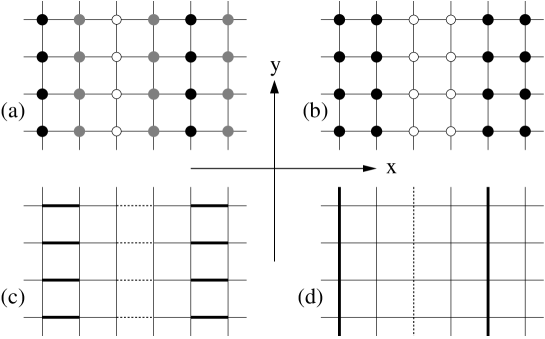
FIG. 1.: Order parameters with wavevector ${\bf Q}=(\frac{2\pi}{4},0)$ considered in this paper. Figures (a) and (b) correspond to site and bond centered CDW respectively. Black circles correspond to sites of higher electron density, white circles to sites of lower electron density, and gray circles to sites with the average electron density. Figures (c) and (d) describe longitudinal and transverse dimerizations respectively. Heavy lines correspond to bonds with higher tunneling amplitude, and dotted lines to bonds with lower tunneling amplitude. Anomalous dimerization may be shown schematically as on figures (c) and (d), with heavy and dotted bonds describing higher and lower pairing amplitudes.

FIG. 2.: Energy dependence of the Fourier component of the local density of states $\rho_{\bf Q}(\epsilon)$ at ${\bf Q}=(2\pi/4,0)$ for various cases of charge ordering. $\rm{Bi_{2}Sr_{2}CaCu_{2}O_{8+\delta}}$ type band structure is assumed. We show a direct calculation based on formulas (16,18,21). The curves correspond to the CDW (solid), longitudinal dimerization (dashed) and anomalous longitudinal dimerization (dotted) orders. To simplify the comparison, $\rho_{\bf Q}(\epsilon)$ is multiplied by $-1$ for CDW, and by $\frac{1}{2}$ for anomalous longitudinal dimerization. In addition, subsequent curves are shifted vertically by 0.6. Results for both kinds of transverse dimerization are qualitatively similar to corresponding longitudinal results and are omitted for visual clarity.

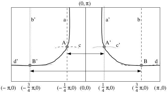
FIG. 3.: Fermi surface for $\rm{Bi_{2}Sr_{2}CaCu_{2}O_{8+\delta}}$ . Dashed lines correspond to the quasiparticles that satisfy $E_{{\bf k}+{\bf Q}}=E_{\bf k}$ and are strongly affected by $\Delta{\cal H}$ when ${\bf Q}=(2\pi/4,0)$. Quasiparticles on line $a$ hybridize with quasiparticles on line $a^{\prime}$ (and similarly for lines $b$ and $b^{\prime}$, and curves $c,$ $c^{\prime}$ and $d,$ $d^{\prime}$). Crossings of these lines with the Fermi surface (points A and A’, B and B’) give the minimal energy of such quasiparticles: $0.5\Delta_{0}$ and $0.7\Delta_{0}$ respectively. Contributions from these points produce sharp peaks at energies $20$ and $30$ meV in Fig. 2. The Van Hove singularity for the Bogoliubov quasiparticles at energy $\Delta_{0}$ leads to a peak at $40$ meV.

FIG. 4.: The results in Fig. 2 are shown after smearing over an energy range of 8 meV. To simplify the comparison, $\rho_{\bf Q}(\epsilon)$ was multiplied by $-1$ for CDW and anomalous transverse dimerization, and by a factor of $-\frac{1}{2}$ for transverse dimerization.

FIG. 5.: $\rho_{Q}(\epsilon)$ for $\rm{Bi_{2}Sr_{2}CaCu_{2}O_{8+\delta}}$ type band structure, ordering wavevector $Q=2\pi/4$ and a combination of charge orders: longitudinal dimerization and CDW, $1.05({\rm CDW})+({\rm long.dim.})$ (solid line); anomalous longitudinal dimerization and CDW, $({\rm anom.long.dim.})+0.2({\rm CDW})$ (long-dashed line). The same smearing is assumed as in Fig.4. For clarity, curves have been offset vertically by 0.25.

FIG. 6.: $\rm{YBa_{2}Cu_{3}O_{6.35}}$ type band structure and ordering wavevector ${\bf Q}=(2\pi/8,0)$. The inset shows $\rho_{Q}(\epsilon)$ for CDW (solid line), dimerization (dashed line), and anomalous dimerization (dotted line) separately. Main figure has the linear combination $({\rm ald})+0.2({\rm CDW})$, which was displayed for $\rm{Bi_{2}Sr_{2}CaCu_{2}O_{8+\delta}}$ in Fig. 5 (the other linear combination is nearly zero and thus omitted). The same smearing is assumed as in Fig. 4.

FIG. 7.: Dispersion in the $(0,0)$ to $(\pi,0)$ direction in a system with charge order with randomness (momentum is measured in units of $2\pi$). Charge order is assumed to have Gaussian distribution centered around wavevector $(2\pi/4,0)$ with the width $2\pi/20$. The function $V({\bf q})$ in (25) is shown, up to a scale, as the thick solid curve. For visual clarity, only results corresponding to the linear combination $1.05({\rm CDW})+({\rm ld})$ are displayed. Each curve corresponds to a different bias; starting from the bottom, the biases are 8 mV, 12 mV, 16 mV, and 20 mV. Throughout, the quasiparticle smearing is fixed at 8 meV.

FIG. 8.: Dispersion in the $(0,0)$ to $(\pi,0)$ direction in a model with impurity induced quasiparticle scattering (momentum is measured in units of $2\pi$). Each curve corresponds to a different bias; starting from the bottom, the biases are 8 mV, 12 mV, 16 mV, and 20 mV. Unlike other computations in this paper, the quasiparticle smearing is fixed at 2 meV. This is done since the main features in these curves are averaged out for the usual smearing of 8 meV.

FIG. 9.: (a) Diagram of Hartree type used in computing the RPA response for a system of interacting electrons in the vicinity of a CDW instability. An external field (e.g. an impurity potential) pins the CDW. (b) and (c) Contributions beyond the Hartree approximation, which may be subdominant depending on the model used. Their inclusion leads to a frequency-dependent self energy.

REFERENCES

- [1] J.E. Hoffman, E. W. Hudson, K. M. Lang, V. Madhavan, H. Eisaki, S. Uchida, J.C. Davis, Science 295, 466 (2002).
- [2] C. Howald, H. Eisaki, N. Kaneko, A. Kapitulnik, cond-mat/0201546.
- [3] J.E. Hoffman, K. McElroy, D.-H. Lee, K.M. Lang, H. Eisaki, S. Uchida, J.C. Davis, Science 297, 1149 (2002).
- [4] K. McElroy, R.W. Simmonds, J.E. Hoffman, D.-H. Lee, J. Orenstein, H. Eisaki, S. Uchida, J.C. Davis, preprint
- [5] C. Howald, H. Eisaki, N. Kaneko, A. Kapitulnik, cond-mat/0208442.
- [6] J. Zaanen and O. Gunnarson, Phys.Rev. B 40, 7391 (1989).
- [7] V. J. Emery, S. A. Kivelson, and J. M. Tranquada, Proc. Natl. Acad. Sci. USA 96, 8814 (1999).
- [8] S.C. Zhang, Science 275, 1089 (1997).
- [9] A. Polkovnikov, S. Sachdev, M. Vojta, E. Demler, Physical Phenomena at High Magnetic Fields IV, October 19-25, 2001, Santa-Fe, New Mexico, cond-mat/0110329
- [10] M. Vojta and S. Sachdev, Phys. Rev. Lett. 83, 3916 (1999)
- [11] S. Chakravarty, R. B. Laughlin, D. K. Morr, C. Nayak, Phys. Rev. B 63, 094503 (2001).
- [12] C. Varma Phys. Rev. Lett. 83, 3538-3541 (1999).
- [13] J. M. Tranquada, J.D. Axe, N. Ichikawa, A.R. Moodenbaugh, Y. Nakamura, S. Uchida, Phys.Rev. Lett. 78, 338 (1997).
- [14] S. Katano, M. Sato, K. Yamada, T. Suzuki, and T. Fukase, Phys. Rev. B 62, R14677 (2000).
- [15] B. Lake, , H.M. Ronnow, N.B. Christensen, G. Aeppli, K. Lefmann , D.F. McMorrow, P. Vorderwisch, P. Smeibidl, N. Mangkorntong , T. Sasagawa, M. Nohara, H. Takagi, T.E. Mason, et.al., Nature 415 299 (2002).
- [16] B. Khaykovich, Y. S. Lee, R. Erwin, S.-H. Lee, S. Wakimoto, K. J. Thomas, M. A. Kastner, R. J. Birgeneau, cond-mat/0112505.
- [17] H.A. Mook, P. Dai, and F. Dogan, Phys. Rev. Lett. 88, 97004 (2002).
- [18] Q.-H. Wang, D.-H. Lee, cond-mat/0205118.
- [19] A. Polkovnikov, S. Sachdev and, M. Vojta, cond-mat/0208334.
- [20] H. Schulz, J. Phys. (Paris) 50, 2833 (1989).
- [21] L. Pryadko et.al. Phys. Rev. B 60, 7541 (1999).
- [22] Y. Zhang, E. Demler, and S. Sachdev, Phys. Rev. B 66, 094501 (2002).
- [23] O. Zachar,S. A. Kivelson, and V. J. Emery, Phys. Rev. B 57, 1422 (1998).
- [24] H.F. Fong, P. Bourges, Y. Sidis, L.P. Regnault, A. Ivanov, G.D. Gu, N. Koshizuka, B. Keimer, Nature 398, 588 (1999).
- [25] A. Polkovnikov, M. Vojta, and S. Sachdev, Phys. Rev. B 65, 220509 (2002).
- [26] H.D. Chen, J.P. Hu, S. Capponi, E. Arrigoni, S.C. Zhang, Phys. Rev. Lett. 89, 137004 (2002).
- [27] H. Mook, P. Dai, F. Dogan, R.D. Hunt, Nature 404, 729 (2000).
- [28] The distinction between site and bond-centered orders is only defined for translational symmetry breaking commensurate with the lattice, i.e. when the wavevector is with integer.
- [29] S. Kivelson, W.-P. Su, J.R. Schrieffer, and A.J. Heeger, Phys. Rev. Lett. 58, 1899 (1987).
- [30] S.A. Kivelson, E. Fradkin, V. Oganesyan, J.M. Tranquada, A. Kapitulnik, and C. Howald, preprint.
- [31] D.S. Marshall, D.S. Dessau, A.G. Loeser, C-H. Park, A.Y. Matsuura, J.N. Eckstein, I. Bozovic, P. Fournier, A. Kapitulnik, W.E. Spicer, and Z.-X. Shen, Phys. Rev. Lett. 76 4841 (1996).
- [32] We only consider spin singlet interactions in (23), since these are the only ones contributing to to linear order in perturbation theory.