Influence of the passive region on Zero Field Steps for window Josephson junctions

Abstract

We present a numerical and analytic study of the influence of the passive region on fluxon dynamics in a window junction. We examine the effect of the extension of the passive region and its electromagnetic characteristics, its surface inductance $L_{I}$ and capacitance $C_{I}$. When the velocity in the passive region $v_{I}$ is equal to the Swihart velocity (1) a one dimensional model describes well the operation of the device. When $v_{I}$ is different from 1, the fluxon adapts its velocity to $v_{I}$. In both cases we give simple formulas for the position of the limiting voltage of the zero field steps. Large values of $L_{I}$ and $C_{I}$ lead to different types of solutions which are analyzed.

I Introduction

The present design of low temperature superconducting devices based on semi-conductor technology enables to integrate Josephson junctions into superconducting strip-lines to realize complex devices. A simple example is the window design shown in Figure 1 where a single rectangular junction is surrounded by a uniform passive region. In other systems like integrated receivers as0 (August 2001), the local flux flow oscillator is coupled directly to a strip-line containing a few junctions which will realize the mixing of the local signal with the external signal coming from an antenna.

The electrodynamic behavior of such window junctions is given by the phase difference between the top and bottom superconducting layers. It obeys an inhomogeneous sine-Gordon equation which is equivalent to a homogeneous sine-Gordon equation for the junction domain coupled to a wave equation for the passive region.
In the static case, a small passive region causes a rescaling of the Josephson length $\lambda_{J}$ into $\lambda_{\rm eff}>\lambda_{J}$ Caputo et al. (1996a) and this renormalization was seen in the experiments by the group of Ustinov Franz et al. (2001). On the other hand a large passive region causes the destruction of the kink due to the finite length of the junction Caputo et al. (1994).

In the dynamical case two limiting systems can be considered, first the passive region can be present only along the longitudinal direction of the junction. Then one can assume a transverse profile that propagates in the long direction. Using these ideas, Lee et al derived the dispersion relation for linear superconducting strip-lines Lee (1991); Lee and Barfknecht (1992). The motion of kinks in such a window junction was studied by one of the authors using periodic boundary conditions in $x$ Flytzanis et al. (2000). It was shown that the speed of the kink depends on the extension of the passive region and that Cerenkov resonances occur between the cavity modes and the kink. These show up as steps in the zero field steps (ZFS) in the IV characteristics. The experiments conducted in this geometry, for a fixed set of electric parameters Barbara et al. (1996) confirm these findings.

In the second limiting case, which we will call the 1D model, the passive region exists only at each end of the junction as shown in the bottom left panel of Figure 1. Then the passive region acts in a different way, and fixes the speed of the kink Benabdallah et al. (2002). In Benabdallah et al. (2002) we also studied the 2D problem i.e. a homogeneous passive region surrounding the junction, using an adapted numerical method, the finite volume approximation together with soliton perturbation theory. The 1D model showed that interfaces can act as fluxon traps. Numerical results in the two dimensional case indicated that the sheet inductance miss-match $L_{I}/L_{J}$ between the junction and the passive region is the main cause of instability of the kink motion.

Here we confirm these results, give the details of the characteristic IV curves and ZFS for the 1D and 2D models and compare these two situations for different geometrical and electrical parameters. We also give a complete derivation of the continuum model used in Benabdallah et al. (2002) from the Resistive Shunted Junction (RSJ) approximation and explain discreteness effects observed in the solution of the 1D model. For the 2D model we justify the fact that the kink adapts its velocity to the one in the passive region. Finally we provide insight into the kink stability for large sheet inductance in the passive region $L_{I}$ or capacitance per unit surface $C_{I}$. In the 2D case we give specifically the different IV curves which can be seen for the different values of the sheet inductance in the passive region $L_{I}$.

The paper is organized as follows. After deriving the continuum equations for the RSJ model in section 1, we introduce the 1D model and study its zero field steps in section 2. In Section 3 we study the ZFS for the 2D model and compare them to the ones for the 1D model. We give our concluding remarks in section 4.

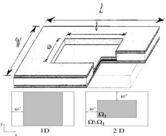
Figure 1: A view of a window Josephson junction. The bottom left panel shows a schematic top view. For the system shown on the right the linear region exists only on the left and right sides of the junction.

Figure 2: Portion of equivalent circuit model corresponding to the window junction displayed in Fig. 1. Crosses represent tunnel elements. The critical curent $I_{i}^{c}$ is nonzero only inside de window

II The model

II.1 RSJ model for window Josephson junction

A simple mathematical model of the window Josephson junction is to describe each superconductor by an array of inductances $L$ (see Fig. 2). The coupling elements between two adjacent nodes in each array are, a capacitor $C$, a resistance $R$ and a Josephson current $I_{c}$ Likharev (1986); Devoret . The Kirchoff laws at each couple of nodes $(i_{b},i_{t})$ in the bottom and top superconducting layers can be combined to give the relation expressing the conservation of currents at node $i$ in the Josephson junction

$$C_{J}\ddot{\Phi}_{i}+\sum_{j}\frac{\Phi_{i}-\Phi_{j}}{L_{ij}}+I_{i}^{c}\sin\frac{\Phi_{i}}{\Phi_{0}}+\frac{\dot{\Phi}_{i}}{R_{i}}=0\;,$$ (1)

and in the passive region

$$C_{I}\ddot{\Psi}_{i}+\sum_{j}\frac{\Psi_{i}-\Psi_{j}}{L_{ij}}=0\;,$$ (2)

where $\Phi=\Phi_{t}-\Phi_{b}$ (resp. $\Psi=\Psi_{t}-\Psi_{b}$), is the phase difference between the two superconductors in the junction (resp. passive) part, the summation $\sum_{j}$ is applied to the nearest neighbors. Also note that equations (1) and (2) are discretisations of Maxwell’s equations (wave equation part) and Josephson constitutive equations (sinus term), assuming an electric field normal to the plates, a magnetic field in the junction plane and perfect symmetry between the top and bottom superconducting layers. We can now obtain the model in the continuum limit, more suitable for analysis.

II.2 Continuum limit

The continuum version of the system (1)-(2) can be derived by introducing the following quantities per unit area ($a^{2}$) of elementary cells of length $a$.

$$\overline{C_{I,J}}=\frac{C_{I,J}}{a^{2}},~{}~{}~{}j_{c}=\frac{I_{i}^{c}}{a^{2}},~{}~{}~{}\overline{r}=Ra^{2}.~{}~{}~{}$$ (3)

We normalize the phases by the flux quantum $\Phi_{0}$,

$$\phi_{i}=\frac{\Phi_{i}}{\Phi_{0}}\quad,\quad\psi_{i}=\frac{\Psi_{i}}{\Phi_{0}}\;,$$ (4)

and introduce the Josephson characteristic length $\lambda_{J}=a\tilde{\lambda_{J}}$

$$\lambda_{J}^{2}=\frac{\phi_{0}}{2\pi j_{c}L_{J}}=\frac{\Phi_{0}}{j_{c}L_{J}}=\tilde{\lambda_{J}}^{2}a^{2}\;.$$ (5)

Notice that in this 2D problem the inductance associated to each cell is equal to the branch inductance $L_{J}$ (resp. $L_{I}$) in the junction (resp. passive region). This is not the case for the 1D model for which these inductances are in series, giving a total inductance proportional to the mesh size $dx$.

We substitute relations (3) - (5) in (1) and (2) and obtain in the junction

$$a^{2}\Phi_{0}\overline{C_{J}}\ddot{\phi}_{i}+\Phi_{0}\sum_{j}\frac{\phi_{i}-\phi_{j}}{L_{ij}}+a^{2}j_{c}\sin\phi_{i}+\frac{a^{2}}{\overline{r}}\Phi_{0}\dot{\phi}_{i}=0\;,$$ (6)

and in the passive part

$$a^{2}\Phi_{0}\overline{C_{I}}\ddot{\psi}_{i}+\Phi_{0}\sum_{j}\frac{\psi_{i}-\psi_{j}}{L_{ij}}=0\;.$$ (7)

After simplification of Eqs. (6)-(7) and using Eq. (5) we obtain

$$\overline{C_{J}}L_{J}\ddot{\phi}_{i}+\sum_{j}\frac{\phi_{i}-\phi_{j}}{a^{2}}+\frac{1}{\lambda_{J}^{2}}\sin\phi_{i}+\frac{L_{J}}{\overline{r}}\dot{\phi}_{i}=0\;,$$ (8)

$$\overline{C_{I}}L_{I}\ddot{\psi}_{i}+\sum_{j}\frac{\psi_{i}-\psi_{j}}{a^{2}}=0\;.$$ (9)

Now we take the limit $a\rightarrow 0$, so that
$\displaystyle{\sum_{j}\frac{\phi_{i}-\phi_{j}}{a^{2}}\rightarrow-\Delta\phi}$  and  $\displaystyle{\sum_{j}\frac{\psi_{i}-\psi_{j}}{a^{2}}\rightarrow-\Delta\psi}$.
and obtain the following system of partial differential equations

$$\overline{C_{J}}L_{J}\frac{\partial^{2}\phi}{\partial t^{2}}-\Delta\,\phi+\frac{1}{\lambda_{J}^{2}}\sin\phi+\frac{L_{J}}{\overline{r}}\frac{\partial\phi}{\partial t}=0\;,$$ (10)

$$\overline{C_{I}}L_{I}\frac{\partial^{2}\psi}{\partial t^{2}}-\Delta\,\psi=0\;.$$ (11)

We introduce the plasma frequency in the junction $\omega_{J}^{-2}=\lambda_{J}^{2}v_{I}^{-2}\;,$ where $v_{I}^{-2}=\overline{C_{J}}L_{J}$ is the Swihart velocity Swihart (1961). Similarly we define the electromagnetic wave frequency in the passive part $\omega_{I}^{-2}=\lambda_{J}^{2}v^{-2}\;,$ where $v^{-2}=\overline{C_{I}}L_{I}$. In the following we fix the couple $(L_{J},C_{J})$ and $\omega_{J}$ and vary the inductance $L_{I}$ and capacity $C_{I}$ in the passive region.
We normalize equations (10) - (11) in space by $\lambda_{J}$ and in time by $\omega_{J}^{-1}$ and obtain in the junction ($\Omega_{J}$)

$$\frac{\partial^{2}\phi}{\partial t^{2}}-\Delta\,\phi+\sin\phi+\alpha\frac{\partial\phi}{\partial t}=0\;,$$ (12)

and in the passive region $(\Omega\backslash\Omega_{J})$

$$\left(\frac{\omega_{J}}{\omega_{I}}\right)^{2}\frac{\partial^{2}\psi}{\partial t^{2}}-\Delta\,\psi=0\;,$$ (13)

where the dimensionless parameter $\alpha=\frac{\tilde{\lambda_{J}}}{R}\sqrt{\frac{L_{J}}{\overline{C_{J}}}}$ is a damping coefficient which depends on the spatial discretization via $\tilde{\lambda_{J}}$.

The boundary conditions of equations (12) and (13) are of inhomogeneous Neumann type which physically indicates a lateral injection of current or/and an external magnetic field

$$\frac{1}{L_{I}}\nabla\psi\cdot n=J_{ext}\;\;{\rm on}\;\;\partial\Omega\;,$$ (14)

where $n$ is the exterior normal. To this we add the interface conditions for the phase and its normal gradient, the surface current on the junction boundary $\partial\Omega_{J}$

$$\psi=\phi~{}~{}~{}{\rm and}~{}~{}~{}{1\over L_{I}}{\partial\psi\over\partial n}={\partial\phi\over\partial n}$$ (15)

Note that the jump condition (2nd relation in (15)) can be obtained by integrating (12) - (13) on a small surface overlapping the junction domain $\Omega_{J}$.
In the rest of the paper we assume a rectangular window of length $l=10$ and width $w=1$ embedded in a rectangular passive region of extension $w^{\prime}$ as shown in Figure 1. We will not consider the influence of an external magnetic field and will assume the external current feed to be of overlap type so that the boundary conditions (14) become

$$\frac{1}{L_{I}}\frac{\partial\psi}{\partial y}(x,0) = -\frac{I}{2{\cal L}},~{}~{}~{}\frac{1}{L_{I}}\frac{\partial\psi}{\partial y}(x,{\cal W})=\frac{I}{2{\cal L}},$$

$$\frac{\partial\psi}{\partial x}(0,y) = \frac{\partial\psi}{\partial x}({\cal L},y)=0,$$ (16)

where ${\cal L}=2w^{\prime}+l\quad{\rm and}\quad{\cal W}=2w^{\prime}+w$.

We assumed throughout the study a small damping $\alpha=0.01$ which is typical of under damped Josephson junctions.

III A 1D window Josephson junction

III.1 The model

We first consider the simplified situation where the passive region is present only at the two lateral ends of the device as shown in the bottom left panel of Fig. 1. For this system it is possible to derive the effective 1D equation Benabdallah et al. (2002)

$$C(x)\varphi_{tt}-\partial_{x}\left(\frac{1}{L(x)}\varphi_{x}\right)+\epsilon(x)( \sin\varphi+\alpha\varphi_{t})-\gamma(x)=0$$ (17)

$${\rm for}~{}~{}x\in]0,{\cal L}[,$$

where $\varphi$ is the phase averaged in y across the junction and $\gamma(x)=\frac{I}{L(x)s}$ where $s$ is the junction area.
In equation (17) $C,L$ and $\epsilon$ are discontinuous functions of $x$ defined by

$$(C(x),L(x),\epsilon(x))=\left\{\begin{array}[]{cc}(1,1,1)&\;\;{\rm if}\;\;x\in]w^{\prime},w^{\prime}+l[\\ \\ (C_{I},L_{I},0)&\;\;{\rm if}\;\;x\in]0,w^{\prime}[\cup]w^{\prime}+l,{\cal L}[\;,\end{array}\right.$$ (18)

The boundary conditions (16) reduce then to

$$\varphi_{x}(0)=\varphi_{x}({\cal L})=0\;.$$ (19)

To compare different values of $w^{\prime}$ we normalize the current $I$ by the maximum current that the junction can carry $I_{\rm max}=s$. To simplify the calculations we have assumed a constant current density $\gamma$.

We choose the values of the inductance $L_{I}$ and capacity $C_{I}$ according to two strategies. First we assume $L_{I}\,C_{I}=v_{I}^{-2}$ is constant which gives a uniform velocity in the passive part. In a second set of calculations we vary $v_{I}$ by moving orthogonally to the set of hyperbolas in the $(L_{I},C_{I})$ plane.

The numerical method to obtain the (IV) curve is to start with a static kink like solution obtained by solving the static problem derived from (17) and to increase progressively the current to obtain a moving fluxon. After obtaining a stable solution in time, we compute the voltage in the center of the junction by

$$V\equiv\frac{1}{T_{2}-T_{1}}\int_{T_{1}}^{T_{2}}\varphi_{t}(w^{\prime}+l/2,t)\;{\rm d}t=$$

$$\frac{\varphi(w^{\prime}+l/2,T_{2})-\varphi(w^{\prime}+l/2,T_{1})}{T_{2}-T_{1}}\,,$$ (20)

where the times $T_{1}$ et $T_{2}$ are given such that the voltage is stable.

III.2 Discreteness effects

In this section we consider a window junction with homogeneous electric properties ($L_{I}=C_{I}=1)$ and fix the width of the passive part $w^{\prime}=2$. We have chosen the number of discretization points in the $x$ direction as $N=253,503,703$ and $1003$. In this case we compute the IV characteristic as shown in the top panel of Fig. 3.

For small values of $N$, we observe resonances in the IV curve which decrease and disappear as the number of mesh points is increased from $N=253$ to 703. These disappear altogether for $N=1003$. To see if these resonances are due to the presence of the passive region, we have calculated a IV curve for a homogeneous junction ($w^{\prime}=0$) and indeed they are absent. To understand the mechanism of this fine structure in the IV curve, we have plotted on the bottom panel of Fig.3 the instantaneous voltage $\phi_{t}$ as a function of $x$ for a fixed time and $N=703,1003$ and $1403$. From the comparison of the two panels of Fig. 3, it is clear that the radiation is responsible for the fine structure. In fact the wave length of the excited radiation corresponds to a standing mode $V=2~{}n\pi/4$ with $n\approx 10$.

Let us now explain how such radiation is excited by the kink as it crosses an interface from a linear to a nonlinear medium. Fig. 4 shows the phase velocity $v_{\phi}=\omega/k$ for the continuum sine-Gordon system (where $\sin\phi\approx\phi$) and the discrete system used numerically for which the second derivative is approximated by a three points difference $\phi_{xx}=(\phi_{n+1}+\phi_{n-1}-2\phi_{n})$. For the former $v_{\phi}=\sqrt{1+1/k^{2}}~{}~{}>~{}~{}1$ so that nonlinear modes cannot be excited via the long wave short wave Benney resonance mechanism Dodd et al. (1982). This is not true for the discrete system for which

$$v_{\phi}={1\over k}\sqrt{1+{4\over h^{2}}\sin^{2}(kh/2)}$$

can be smaller than 1 for $h\neq 0$ and small wave lengths. As expected the threshold $k$ decreases as is increased. Notice that the scale in $k$ corresponds to $9\times\pi/2\leq k\leq 12\times\pi/2$.

We then explain quantitatively the resonances in the IV curve shown in Fig. 3 by the fact that as the kink velocity increases, it can lock with a given cavity mode. For example $N=703$ gives voltage (resp. velocity) steps $V=0.4457,0.44645,0.447,0.4475$ (resp. $v=0.9935,0.9952,0.996,0.997)$ which correspond to the cavity mode index $n=14,13,12$ and $11.$ For $N=503$ we observe steps at voltages $V=0.4451,0.446,0.4467$ (resp. $v=0.9922,0.99426,0.9958)$ for which $n=11,10$ and $9$ respectively. The lower values of $n$ explain the larger amplitudes observed in the radiation.

An intrinsic fine structure in the IV characteristics has been seen in experiments with window junctions with a lateral passive region. For example Thyssen et al. in Parmentier and Pedersen (1995) show a slight shift in the position (and therefore limiting fluxon velocity) of the IV curves for different values of $w^{\prime}$. Ustinov et al Barbara et al. (1996) also display IV curves which depend on $w^{\prime}$ and large substructures. Recent numerical work Flytzanis et al. (2000) on a Josephson window junction with a lateral passive region and periodic boundary conditions along the propagation direction confirm these resonances due to Cerenkov radiation between a soliton travelling faster than $v=1$ and the radiation of phase speed $v_{\phi}=\sqrt{1+1/k^{2}}>1$. Here we show that when the passive region exists only in the propagation direction, resonances disappear at large resolutions. This can be expected from the calculation of the emitted power of radiation for a kink as it crosses an interface Kivshar and Chubykalo (1991); Kivshar and Malomed (1989). This quantity drops fast to zero as the speed approaches 1.

Figure 3: 1D dynamics. The top panel shows the current voltage characteristic for $w^{\prime}=2$ and various number of discretization points. The bottom panel shows the corresponding instantaneous voltage $\varphi_{t}(x)$ for a given time for three different values of the discretization $N=703,1003$ and $1403$. The current density is equal to $0.08$.

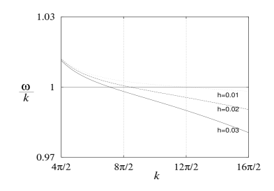
Figure 4: Phase velocity of linear waves for the discrete model $v_{\varphi}$ vs. $k$ for three values of the step discretization $h=0.01,~{}0.02$ and $h=0.03$

In the rest of the study we have chosen $N=1403$ so that numerical resonances are eliminated from the IV characteristic.

III.3 Zero field steps (ZFS)

We now proceed to give an estimate of the time average of the voltage for the window junction. For this, we compute the velocity in the junction using the McLaughlin-Scott soliton perturbation equations McLaughlin and Scott (1978) and get for the kink velocity

$$v=\frac{1}{\sqrt{1+\left(\frac{4\alpha}{\pi\gamma}\right)^{2}}}\;.$$

When the current $\gamma$ increases and becomes larger than $\alpha$, the velocity $v$ gets close to 1.
In the passive part the velocity $v_{I}$ is given by (17)

$$v_{I}=\frac{1}{\sqrt{L_{I}\,C_{I}}}\;,$$

so that the average of the voltage in time in the limit of large current can be approximated by

$$V_{\rm 1D}\equiv<\varphi_{t}>={{\Delta\varphi}\over{\Delta t}}=\frac{2\pi}{2w^{\prime}/v_{I}+l/v}\;,$$ (21)

where the denominator is just the time take by the kink (phase jump of $2\pi$) to travel across the device. We now confirm this estimation first when the electric properties of the device are homogeneous and then when they are different in the junction and the passive region so that $v_{I}\neq 1$.

III.4 Influence of geometry

First we consider a situation where the electric properties are homogeneous in the whole device so that $(L_{I}=C_{I}=1)$ and change the extension of the passive region $w^{\prime}$.
In Fig. 5 we plot the (IV) characteristic curves for four values of $w^{\prime}=0,1,2$ and $3$. This figure. show that the position of the ZFS moves towards the left when $w^{\prime}$ increases. This agrees with formula (21). Table (1) reports the limiting values of the zero field steps and the estimates from (21), which are in excellent agreement. For large value of $w^{\prime}$ (typically $w^{\prime}=12$), the kink becomes unstable. This seems to be due to the fixed points that exist on each junction/passive region interface Benabdallah et al. (2002). The kink can be trapped easier by one of them as $w^{\prime}$ increases because the driving force due to the current gets weaker.

Figure 5: The 1D current voltage characteristic for $L_{I}=C_{I}=1$ and various extensions of the passive region $w^{\prime}$.

Table 1: positions of the ZFS for the 1D window model homogeneous $(L_{I}=C_{I}=1)$ together with the estimates (21).

$w^{\prime}$	$V_{\rm 1D}$	$V_{\rm num}$1D
$0$	$0.628$	$0.625$
$1$	$0.523$	$0.521$
$2$	$0.448$	$0.447$
$3$	$0.392$	$0.391$

III.5 Influence of the electrical parameters

The second case tested is when the velocity in the passive region $v_{I}\neq 1$. To simplify things we fix $w^{\prime}$ to $2$ in all the presented runs. We show in Fig. 6 the IV characteristics for four values of the velocity in the passive region $v_{I}=0.33,0.5,1$ and $2$. Notice that the positions of the ZFS of the 1D effective model follow (21) as shown in table (2). Fig. 6 also shows that the position of the ZFS moves from the right to the left as $v_{I}$ decreases from $2$ to $0.33$. When $v_{I}$ goes to zero so that $L_{I}$ or $C_{I}$ goes to infinity, we expect the ZFS to disappear. We observe regions of instability for $L_{I}>>1$ or $C_{I}>>1$ and the zero field steps exist only in small intervals in the $(L_{I},C_{I})$ plane. In Fig. 8 we present a detailed numerical exploration of the $(L_{I},C_{I})$ plane. The hyperbolas corresponding to $L_{I}\,C_{I}={v_{I}}^{-2}$ constant are shown. We indicate by the symbols $(*),$ $(\times)$ and $(+)$ the points where the ZFS exist. We note that for these points the solution of the window 1D problem is a kink. The region of stability is concentrated along the diagonal. Note that the results of Fig. 8 are based only on the numerics.
When $C_{I}$ or $L_{I}$ become large we obtain particular types of solutions which we now discuss.

Figure 6: The 1D Current voltage characteristic for $w^{\prime}=2$ and various velocity in the passive region. The velocities $v_{I}$ are indicated in the top right corner of the picture.

Table 2: positions of the ZFS for the 1D window model together with their corresponding estimates (21) for $w^{\prime}=2$.

$L_{I}\,C_{I}$	$v_{I}$	$V_{\rm 1D}$	$V_{\rm num}1D$
$0.25$	2	$0.523$	$0.521$
$1$	1	$0.449$	$0.448$
$4$	0.5	$0.349$	$0.348$
$9$	0.33	$0.285$	$0.284$

III.6 Solutions for large $L_{I}$ or $C_{I}$

Instabilities of the kink motion occur when the extension of the passive region $w^{\prime}$ is large, typically $w^{\prime}\approx 12$. In that case the current density becomes small and cannot drive the kink out of the potential well created by the interface Benabdallah et al. (2002). Other instability factors are the electrical parameters $(L_{I},C_{I})$. We have shown in Benabdallah et al. (2002); Benabdallah (1999) that the electrical parameters act differently from the geometry. For $C_{I}>>1$ the solution is static while it is dynamic for $L_{I}>>1$. In this latter case, kink motion is possible only in the junction.

We now consider the disappearance of the Zero field steps in the $IV$ curves. This occurs for intermediate values of $C_{I}$ and $L_{I}$ and gives rise to a large voltage.

Let us recall the equations of the problem

$$\frac{\partial^{2}\phi}{\partial t^{2}}-\frac{\partial^{2}\phi}{\partial x^{2}}+\sin\phi=\gamma-\alpha\frac{\partial\phi}{\partial t}\quad w^{\prime}\leq x\leq w^{\prime}+l\;,$$ (22)

$$C_{I}\frac{\partial^{2}\psi}{\partial t^{2}}-{1\over L_{I}}\frac{\partial^{2}\psi}{\partial x^{2}}=\gamma~{}~{}~{}0\leq x\leq w^{\prime}~{}~{}{\rm and}~{}~{}w^{\prime}+l\leq x\leq{\cal L}\;,$$ (23)

together with the interface condition at $x=w^{\prime},w^{\prime}+l$

$$\phi=\psi~{}~{}~{},{1\over L_{I}}\frac{\partial\psi}{\partial x}=\frac{\partial\phi}{\partial x}~{}~{},$$

and homogeneous boundary conditions $\frac{\partial\psi}{\partial x}|_{x=0}=\frac{\partial\psi}{\partial x}|_{x={\cal L}}=0$.

In the limit of large voltages $V$

$$\frac{\partial\phi}{\partial t}\approx V~{}~{}~{}{\rm and}~{}~{}~{}\frac{\partial\psi}{\partial t}\approx V$$

so that one can average the above equations which then reduce to

$$-\frac{\partial^{2}\phi}{\partial x^{2}}=\gamma-\alpha V\quad w^{\prime}\leq x\leq w^{\prime}+l\;,$$ (24)

$$-{1\over L_{I}}\frac{\partial^{2}\psi}{\partial x^{2}}=\gamma~{}~{}~{}0\leq x\leq w^{\prime}~{}~{}{\rm and}~{}~{}w^{\prime}+l\leq x\leq{\cal L}\;,$$ (25)

where the voltage $V=\gamma{\cal L}/(\alpha l)$ can be derived from the work equation (see Appendix).

The time dependent part of $\phi,\psi$ is now just $Vt$ and the $x$ dependent part verifies a boundary value problem with $\psi_{x}|_{x=0,{\cal L}}=0$ and the above given interface conditions. The solution is symmetric with respect to $x={\cal L}/2$ and we obtain for the left and right passive regions and the junction

$$\psi_{l}=-\gamma L_{I}{x^{2}\over 2}+Vt,$$ (26)

$$\psi_{r}=-\gamma L_{I}{({\cal L}-x)^{2}\over 2}+Vt$$ (27)

$$\phi=-\gamma{w^{\prime}\over l}x({\cal L}-x)+\gamma{{w^{\prime}}^{2}\over 2}(2-L_{I}+{2w^{\prime}\over l})+Vt$$ (28)

The above given expressions give a very good approximation of the phase computed numerically as can be seen in Fig. 7 which shows $\psi(x)$ and $\phi(x)$ for 11 successive values of time. The electrical parameters are $C_{I}=1~{}~{},L_{I}=10$ and the top panel corresponds to a small current density $\gamma=0.1$ while the bottom panel is for $\gamma=0.25$. The agreement for the latter is excellent, showing complete overlap between the approximation (26,27,28) and the numerical solution. On the top panel the approximations give the overall value but there are some oscillations due to a resonance between the main frequency $V$ and a subharmonic.

It is possible to estimate the validity of the approximate solution (26,27,28) by considering perturbations around it. This leads to the linearized equations for the perturbations $\xi,\zeta$.

$$\frac{\partial^{2}\xi}{\partial t^{2}}-\frac{\partial^{2}\xi}{\partial x^{2}}+\xi\cos\phi+\alpha\frac{\partial\xi}{\partial t}=0\quad w^{\prime}\leq x\leq w^{\prime}+l\;,$$ (29)

$$C_{I}\frac{\partial^{2}\zeta}{\partial t^{2}}-{1\over L_{I}}\frac{\partial^{2}\zeta}{\partial x^{2}}=0~{}~{}~{}0\leq x\leq w^{\prime}~{}~{}{\rm and}~{}~{}w^{\prime}+l\leq x\leq{\cal L}\;$$ (30)

with the interface condition at $x=w^{\prime},w^{\prime}+l$

$$\xi=\zeta~{}~{}~{},{1\over L_{I}}\frac{\partial\zeta}{\partial x}=\frac{\partial\xi}{\partial x}~{}~{},$$

and boundary conditions $\frac{\partial\zeta}{\partial x}|_{x=0}=\frac{\partial\zeta}{\partial x}|_{x={\cal L}}=0$.

We then assume a uniform time dependence $e^{-\alpha t/2+i\omega t}$ and obtain a spectral problem which can be solved. We can neglect the damping because it is small.

In the particular case presented in the top panel of Fig. 7 the voltage is $V=14$ and the subharmonic observed is $V/4=3.5$. This corresponds to the mode $n_{J}=11$ in the junction and $n_{I}=7$ in each lateral passive region of extension 2, taking into account the inductance $L_{I}=10$.

Figure 7: Phase $\varphi$ versus $x$ for eleven successive times separated by $\Delta t=0.11$. The parameters are $C_{I}=1$, $L_{I}=10$, $\gamma=0.1$ $V=14.$ (top panel) and $\gamma=0.25$, $V=35.$ (bottom panel). The numerical results are given in solid lines while the analytic expression (26,27,28) are given in dashed lines.

Fig. 8 shows the regions of existence of ZFS in the $(L_{I},C_{I})$ plane. Notice the symmetry. For $C_{I}>>1$ the solution is static while it is dynamic for $L_{I}>>1$, this latter parameter plays a predominant role due to the interface conditions.

Figure 8: Parameter plane $(L_{I},C_{I})$ showing the regions of existence of zero field steps (ZFS) corresponding to the shuttling motion of a fluxon in the 1D case. The velocities $v_{I}$ are indicated in the top right corner of the picture.

IV 2D window junction

In this section we discuss the dynamics of the kink in the window junction and how to reduce it to a 1D effective problem. It is known that for a pure Josephson junction this reduction is possible. For example in the static case the behavior of a junction of width $w<2\pi$ is very well approximated by the equation for the zero order mode Caputo et al. (1996b). For the dynamical case Eilbeck et al. Eilbeck et al. (1985) found that when $(I/{8{\cal L}}\ll 1)$ the phase is uniform in the $y$ direction so that the reduction is possible. For a window junction the situation is different because we have a passive region around the junction which has electrical properties, a capacity and an inductance which fix the velocity $v_{I}$. The comparison between 2D and 1D was done for the two cases of homogeneous electrical properties in different geometries and a fixed geometry with different electrical properties. Before giving these results we discuss how the kink velocity is fixed by the presence of the passive region.

IV.1 Justification of the effective 1D model

When the velocity in the passive region $v_{I}\neq 1$ the formula (21) is completely off for the 2D calculations and the reduction of the 2D window junction problem to a 1D effective problem is impossible.
Here the lateral passive region where waves can only propagate at velocity $v_{I}$ is controlling the kink motion. The velocity -a free parameter for the sine-Gordon equation- can then adjust itself to $v_{I}$ so that the ”dressed” kink can propagate in the device (junction and lateral passive region). The fluxon adapts its velocity to $v_{I}$ so that $v=v_{I}$.

To justify this, we take the time derivative of the first interface condition (15) and obtain

$$\phi_{t}=\psi_{t}~{}~{}~{}{\rm on}~{}~{}~{}\partial\Omega_{J}\;,$$ (31)

the second interface condition (15) reads

$$\nabla\phi\cdot n=\nabla\psi\cdot n\quad{\rm on}\quad\partial\Omega_{J}\;.$$ (32)

The numerical simulations show that it is legitimate to assume that the solution is a 1D kink travelling in the passive region with the velocity $v_{I}$ and in the junction with velocity $v$. Then (32) becomes at the longitudinal boundaries

$$\partial_{x}\phi=\partial_{x}\psi~{}~{}~{}{\rm on}~{}~{}~{}\partial\Omega_{J}\;.$$ (33)

The velocity $v$ of the kink on the boundary of the junction is defined by

$$v=-\frac{\phi_{t}}{\phi_{x}}~{}~{}~{}{\rm on}~{}~{}~{}\partial\Omega_{J}\;.$$ (34)

and the same for the velocity $v_{I}$ of the linear wave on the boundary of the junction

$$v_{I}=-\frac{\psi_{t}}{\psi_{x}}~{}~{}~{}{\rm on}~{}~{}~{}\partial\Omega_{J}\;.$$ (35)

Thus from (31) and (33) we obtain $v=v_{I}$ so that the estimate for the average voltage is then

$$V_{\rm 2D}=\frac{2\pi}{2w^{\prime}/v_{I}+l/v_{I}}$$ (36)

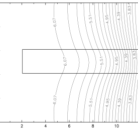
Figure 9: Contour of the phase for a homogeneous window junction with $w^{\prime}=2$ and $I=0.22$

IV.2 Influence of the geometry on the zero field steps

In this case the electrical properties are homogeneous in the whole device so that ($L_{I}=C_{I}=1$). The numerical simulations show that for different $w^{\prime}$ the solution of the 2D problem are $y-$ uniform. For $w^{\prime}=2$ for example the Fig. 9 represent the contour of the phase in the whole domain at the time $T=5.024\,10^{4}$. We note that the Fig. 9 was normalized by ${\rm max}|\phi|$. The levels lines are parallel in the $y$ direction so that the solution is very close to a 1D kink. This 1D kink propagates with a velocity $v_{I}$.

Figure 10: Current voltage characteristic for a homogeneous window junction and various extensions of the passive region $w^{\prime}$. Both 1D and 2D calculations are presented for comparison.

The figure (10) shows the IV characteristics for the both 1D and 2D problems. One can see the good agreement between the 1D and 2D calculations. Table (3) reports the limiting values of the zero field step computed numerically and the corresponding estimates from (21) in excellent agreement.
As the numerical results show, in this case the dynamics of the solution in the 2D window problem can be described by a unidimensional fluxon and the reduction to a 1D effective problem is possible.

Table 3: positions of the ZFS for a both 1D and 2D homogeneous junction together with the estimates (21).

$w^{\prime}$	$V_{\rm 1D}$	$V_{\rm num}$1D	$V_{\rm num}$2D
$0$	$0.628$	$0.625$	$0.606$
$1$	$0.523$	$0.522$	$0.510$
$2$	$0.449$	$0.448$	$0.442$
$3$	$0.392$	$0.391$	$0.386$

IV.3 Influence of the electrical parameters

We have obtained the same average voltage for different values of $L_{I}\,C_{I}$ as long as the product $L_{I}~{}C_{I}=v_{I}^{-2}$ is kept constant. We observe that the position of the zero field step moves from the right to the left as the velocity in the passive region $v_{I}$ decreases from $2$ to $0.5$. We expect the ZFS to disappear when $v_{I}$ goes to $0$ ie $L_{I}$ or $C_{I}$ go to infinity.

IV.4 Instabilities

As in 1D case there are two types of instabilities of the kink. The first is due to the geometry of the window, because large widths $w^{\prime}$ of the passive region (typically $w^{\prime}=7$) lead to a ”stretched” kink in the junction which strongly radiates. It is the impossible to accelerate such an object and have a stable zero field step Benabdallah et al. (2002). This solution which is almost uniform in the junction will oscillate but not rotate and the average voltage will be zero Benabdallah et al. (2002). This situation was observed in the experimental work of Thyssen et al. Parmentier and Pedersen (1995) who never found any zero field step for $w^{\prime}/w<3$.

The second type of instability is due to the electrical quantities $L_{I}$ and $C_{I}$. For $w^{\prime}=2$, we have investigated the $(L_{I},C_{I})$ plane and found numerically the regions of instability of the kink as shown in Fig. 11. We also plot three hyperbolas corresponding to $v_{I}=0.5(*),1(\times)$ and $2(+)$. The markers indicate the positions where we have found the ZFS. All the points for a given marker correspond to the same voltage. In Fig. 11 we have isolated the stability region as the interior of the domain bounded by the solid line. We observe that the instability is due essentially to the inductance $L_{I}$ so that the kink motion is stable for $0.1\leq L_{I}\leq 2$, independently of $C_{I}$. For example $C_{I}=10^{4}$ and $L_{I}=1$ gives rise to a ZFS. We can estimate the average voltage using formula (36), ($V_{\rm 2D}=4.5\times 10^{-3}$ which is very close to the value found numerically $V_{\rm num}2D=4.577\times 10^{-3}$). Thus even for such a large value of $C_{I}$, the formula (36) gives a good agreement with the numerical calculation.
Small values of $C_{I}$ lead to a static solution as can be seen from equation (13) which reduces to $\Delta\psi=0$ so that $\psi$ is constant. Because of the interface conditions $\phi$ is also constant.

The influence of the inductance $L_{I}$ has been analyzed in detail by calculating IV characteristics for $w^{\prime}=3$ and $0.1\leq L_{I}\leq 3$ which are plotted in Fig. 12. There are three main regions identified by the letters A B and C which correspond to three different dynamical behaviors. In region A $2\leq L_{I}\leq 3$, we obtain a static solution and a zero voltage. At this time we do not understand why the kink motion becomes unstable for $L_{I}\geq 2$ independently of $C_{I}$. This effect is present only in two dimensions and therefore linked to the presence of a lateral passive region. It may be due to the large jump in the gradient $\phi_{y}=(1/L_{I})\psi_{y}$ along the lateral interface.
Region B corresponds to a ZFS thus a stable kink motion in the device. The limiting voltage is given to a very good approximation by formula (36) as shown by the inset of Fig. 12. This expression also gives a good estimate even for $v_{I}>1$. Region C $L_{I}=0.1,0.2$ corresponds to much larger values of the voltage and a straight behavior typical of linear resonances in the junction cavity. Small values of $L_{I}$ give rise to a spatially uniform phase in the passive region, which reacts to the phase in the junction. The voltage for $L_{I}=0.1$ corresponds to a higher order cavity mode $V=2.56\approx 6\pi/10$. Fig. 13 shows the corresponding phase at a given instant (top panel) together with the temporal behavior (bottom panel). As expected the phase is almost uniform, the bounds in Fig. 13 are 191.83 and 193.14. The phase increases linearly with time.

Then we conclude that the region of stability of the kink in the window problem is

$$D_{\rm stability}=\{0.1\leq L_{I}\leq 2~{}~{}~{}{\rm and}~{}~{}~{}C_{I}\geq 0.5\}\,.$$ (37)

Figure 11: Parameter plane $(L_{I},C_{I})$ showing the regions of existence of zero field steps (ZFS) corresponding to the shuttling motion of a fluxon for 2D case. The velocities $v_{I}$ are indicated in the top right corner of the picture. The parameter $w^{\prime}=2$

Figure 12: IV characteristics for $0.1\leq L_{I}\leq 3$, $C_{I}=1$ and $w^{\prime}=3$. The insert shows the fluxon velocity in region B as a function of the linear wave speed $v_{I}$ in the passive region.

Figure 13: Three dimensional view of the phase at a given time (t=30800.) for $L_{I}=0.1$, region C in the previous picture (top panel). The bottom panel gives the temporal behavior of the phase in the middle of the junction.

V Conclusion

In this paper we have investigate the electrodynamics of a uniform window junction, using the limiting case termed 1D model where the lateral extension of the passive region is neglected. We use the solution of the 1D model as a guide to discuss the behavior of the full window junction and this enables us to give an estimate of the average voltage for different extensions $w^{\prime}$ of the passive region and different electrical parameters which fix the velocity in the passive region $v_{I}$. This estimate is in excellent agreement with the numerical results even when $v_{I}\neq 1$. In this situation we show that the fluxon adapts its velocity to $v_{I}$. For both cases $v_{I}=1$ and $v_{I}\neq 1$ the numerical results show that the fluxon propagates perpendicularly to the direction of the junction. We have doubled the junction length to $l=20$ and find the same estimates for the limiting voltage. In the 2D window junction, the translational symmetry is broken so that we obtain a different result from the case where only a lateral passive region exists.

We have also studied numerically the stability of the zero field step in the window junction and show that when the width of the passive part becomes large the fluxon becomes distorted and gives to another type of solution which is radial. In this case we have not found any ZFS.

This study shows that the kink can travel into the passive region even when the impedance is not adapted as long as the mismatch is in the capacitance and not the inductance. In other words the limit $\epsilon\rightarrow 0$ is not a singular limit. On the other hand if there is an inductance mismatch then this will most likely cause the break-up of kink shuttling leading to the disappearance of the zero field step. The stability of the fluxon depends essentially on the inductance $L_{I}$. This result, we believe, can lead to improving Josephson devices and their coupling to micro-strip lines.

Acknowledgements It is with great pleasure that J. G. C. thanks N. Flytzanis for many useful discussions at the beginning of this work. A. B. thanks the Laboratory of Mathematics of the INSA de Rouen and the Laboratoire de Physique théorique de l’Université de Cergy-Pontoise for support. A. B. and J. G. C. thank Vladislav Kurin and Alexei Ustinov for many useful electronic exchanges. We thank Jérôme Dorignac for useful discussion. This work was supported by the European Union under the RTN project LOCNET HPRNCT-1999-00163.

Appendix A Derivation of the linear part of the $IV$ curve

To determine the Hamiltonian associated with the 1D-window junction equation we multiply Eq. (17) by $\partial\varphi/\partial t$ and integrate between $0$ and ${\cal L}$ to obtain

$${{\rm d}\over{{\rm d}t}}\left[\int_{0}^{\cal L}\frac{C(x)}{2}\varphi_{t}^{2}+\epsilon(x)\left(1-\cos\varphi\right)\;{\rm d}x\right]$$

$$-\int_{0}^{\cal L}\partial_{x}\left[{1\over{L(x)}}\varphi_{x}\right]\varphi_{t}\;{\rm d}x=\int_{0}^{\cal L}\gamma(x)\varphi_{t}\;{\rm d}x-$$

$$\alpha\int_{0}^{\cal L}\epsilon(x)\varphi_{t}^{2}\;{\rm d}x\;,$$

Integrating by parts the second term in the left-hand side and using the boundary conditions we obtain

$${{\rm d}\over{{\rm d}t}}\left[\int_{0}^{\cal L}\frac{C(x)}{2}\varphi_{t}^{2}+\frac{1}{2L(x)}\varphi_{x}^{2}+\epsilon(x)\left(1-\cos\varphi\right)\;{\rm d}x\right]$$

$$=\int_{0}^{\cal L}\gamma(x)\varphi_{t}\;{\rm d}x-\alpha\int_{0}^{\cal L}\epsilon(x)\varphi_{t}^{2}\;{\rm d}x\;.$$

Recalling the sine-Gordon-wave Hamiltonian

$$H=\int_{0}^{\cal L}\left[\frac{C(x)}{2}\varphi_{t}^{2}+\frac{1}{2L(x)}\varphi_{x}^{2}+\varepsilon(x)\left(1-\cos\varphi\right)\right]\;{\rm d}x$$ (38)

The computation of the linear part of the $IV$ curve is based on the conservation of the energy of the system that is given by sG-wave Hamiltonian (38) from which it can be shown that $H$ satisfies the power balance equation

$${{\rm d}H\over{{\rm d}t}}=\gamma\int_{0}^{\cal L}\varphi_{t}\;{\rm d}x-\alpha\int_{w^{\prime}}^{w^{\prime}+l}\varphi_{t}^{2}\;{\rm d}x$$ (39)

In the stationary regime the average $dH/dt=0$ , so

$$\left<\gamma\int_{0}^{\cal L}\varphi_{t}\;{\rm d}x\right>-\alpha\left<\int_{w^{\prime}}^{w^{\prime}+l}\varphi_{t}^{2}\;{\rm d}x\right>=0\,.$$

Since the voltage $V$ is the temporal average of $\varphi_{t}$, we obtain in the high voltage limit $\left<\varphi_{t}^{2}\right>=\left<\varphi_{t}\right>^{2}$, so that the IV curve is given by

$$V=\frac{\gamma{\cal L}}{\alpha l}$$

References

- as0 (August 2001) Proceedings of the 5th European conference on applied superconductivity (August 2001).
- Caputo et al. (1996a) J. G. Caputo, N. Flytzanis, and M. Vavalis, Int. J. Mod. Phys. C 7, 191 (1996a).
- Franz et al. (2001) A. Franz, A. Wallraff, and A. V. Ustinov, J. Appl. Phys. 89, 471 (2001).
- Caputo et al. (1994) J. G. Caputo, N. Flytzanis, and M. Devoret, Phys. Rev. B 50, 6471 (1994).
- Lee (1991) G. S. Lee, I.E.E.E. Trans. Appl. Superconductivity 1, 121 (1991).
- Lee and Barfknecht (1992) G. S. Lee and A. T. Barfknecht, I.E.E.E. Trans. Appl. Superconductivity 2, 67 (1992).
- Flytzanis et al. (2000) N. Flytzanis, N. Lazarides, A. Chiginev, V. Kurin, and J. G. Caputo, J. Appl. Phys. 88, 4201 (2000).
- Barbara et al. (1996) P. Barbara, R. Monaco, and A. V. Ustinov, J. Appl. Phys. 79, 327 (1996).
- Benabdallah et al. (2002) A. Benabdallah, J. G. Caputo, and N. Flytzanis, Physica D 161, 79 (2002).
- Likharev (1986) K. K. Likharev, Dynamics of Josephson junctions and circuits (Gordon and Breach, 1986).
- (11) M. Devoret, private communication.
- Swihart (1961) J. C. Swihart, J. Appl. Phys 32, 461 (1961).
- Dodd et al. (1982) R. K. Dodd, J. C. Eilbeck, J. D. Gibbon, and H. C. Morris, Solitons and nonlinear wave equations (Academic Press., N.Y., 1982).
- Parmentier and Pedersen (1995) R. D. Parmentier and N. F. Pedersen, eds., Nonlinear superconducting devices and hight materials (World Scientific, 1995).
- Kivshar and Malomed (1989) Y. Kivshar and B. Malomed, J. Appl. Phys. 65, 879 (1989).
- Kivshar and Chubykalo (1991) Y. Kivshar and O. Chubykalo, Phys. Rev. B 43, 5419 (1991).
- McLaughlin and Scott (1978) D. W. McLaughlin and A. C. Scott, Phys. Rev. A. 18, 1652 (1978).
- Benabdallah (1999) A. Benabdallah, Ph.D. thesis, University of Rouen (1999).
- Caputo et al. (1996b) J. G. Caputo, Flytzanis, Y. Gaididei, and M. Vavalis, Phys. Rev. E 54, 2092 (1996b).
- Eilbeck et al. (1985) J. C. Eilbeck, P. S. Lomdahl, O. H. Olsen, and M. R. Samuelsen, J. Appl. Phys. 57, 861 (1985).