Transport properties in the $d$-density wave state: Wiedemann-Franz law

Wonkee Kim and J. P. Carbotte Department of Physics and Astronomy, McMaster University, Hamilton, Ontario, Canada, L8SΒ 4M1
Abstract

We study the Wiedemann-Franz (WF) law in the $d$-density wave (DDW) model. Even though the opening of the DDW gap $(W_{0})$ profoundly modifies the electronic density of states and makes it dependent on energy, the value of the WF ratio at zero temperature $(T=0)$ remains unchanged. However, neither electrical nor thermal conductivity display universal behavior. For finite temperature, with $T$ greater than the value of the impurity scattering rate at zero frequency $\gamma(0)$ i.e. $\gamma(0)<T\ll W_{0}$, the usual WF ratio is obtained only in the weak scattering limit. For strong scattering there are large violations of the WF law.

pacs:
74.25.Fy, 74.20.Fg, 74.20.De

In a recent paper Hill et al. hill have observed large violation of the Wiedemann-Franz (WF) law in (Pr,Ce)2CuO2 driven into the normal state through the application of a $13$ Tesla magnetic field. At very low temperature $T<0.2K$, the thermal conductivity is found to be much less than the value estimated from the D.C. conductivity. Above $0.3K$ the opposite holds. This observation suggests that an exotic state of matter may exist in the normal state of (Pr,Ce)2CuO2. Hill et al. consider spin-charge separation as one possibility.

Recently $d$-density wave (DDW) order has received considerable attention chakravarty1 ; chakravarty2 ; dhlee ; zhu ; kim as a possible exotic state of matter with a pseudogap which breaks time reversal symmetry because it introduces bond current with attendant small orbital magnetic moments. The pseudogap has $d$-wave symmetry. This is the symmetry observed in studies of the variation of the leading edge of the electron spectral density by angle-resolved photoemission spectroscopy, arpes as a function of angle in the Brillouin zone in the normal state of underdoped cuprates. A pseudogap with $d$-wave symmetry implies important energy dependence of the quasiparticles density of states (DOS) at the Fermi surface (FS). Energy dependence in the DOS leads to impurity scattering rates that also depend on energy and the applicability of the usual WF law is no longer guaranteed.

In this paper we consider the WF law within the DDW model. As yet, this model has not been shown to apply to the pseudogap regime of the cuprates. Here we take the point of view that nevertheless it can serve to understand, in this concrete case, how energy dependence in the DOS can alter the WF law.

In the DDW state, the gap with magnitude $W_{0}$ has $d$-wave symmetry and opens up at the antiferromagnetic Brillouin zone of the CuO2 plane. Away from half filling, in the underdoped regime, the FS falls at the chemical potential $\mu$ (which would be zero at half filling) and we assume that $|\mu|\ll W_{0}$. Provided that the effective impurity scattering rate and temperature are also small as compared with $W_{0}$, a nodal approximationdurst can be used to describe the electric as well as the thermal conductivity.

We consider a tight binding energy dispersion as a function of momentum ${\bf k}$ of the form: $\epsilon_{\bf k}=-2t_{0}[\cos(k_{x})+\cos(k_{y})]$, where $t_{0}$ is the in-plane hopping amplitude. At half filling the FS coincides with the antiferromagnetic boundary where the DDW gap $W_{\bf k}=(W_{0}/2)[\cos(k_{x})-\cos(k_{y})]$ opens up with amplitude $W_{0}$. Most properties of the DDW state are determined by the nesting vector ${\bf Q}=(\pi,\pi)$, for example $\epsilon_{{\bf k}+{\bf Q}}=-\epsilon_{\bf k}$ and $W_{{\bf k}+{\bf Q}}=-W_{\bf k}$. See Ref.zhu ; kim for detailed properties.

We begin with the Hamiltonian

$\displaystyle H=$ βˆ«π‘‘π±β€‹ΟˆΞ±β€ β€‹(𝐱)​(βˆ’βˆ‡22​m)β€‹ΟˆΞ±β€‹(𝐱)differential-d𝐱subscriptsuperscriptπœ“β€ π›Όπ±superscriptβˆ‡22π‘šsubscriptπœ“π›Όπ±\displaystyle\int d{\bf x}\psi^{\dagger}_{\alpha}({\bf x})\left(-\frac{\nabla^{2}}{2m}\right)\psi_{\alpha}({\bf x})
$\displaystyle+$ 12β€‹βˆ«π‘‘π±β€‹π‘‘π²β€‹ΟˆΞ±β€ β€‹(𝐱)β€‹ΟˆΞ²β€ β€‹(𝐲)​V​(π±βˆ’π²)β€‹ΟˆΞ²β€‹(𝐲)β€‹ΟˆΞ±β€‹(𝐱),12differential-d𝐱differential-d𝐲subscriptsuperscriptπœ“β€ π›Όπ±subscriptsuperscriptπœ“β€ π›½π²π‘‰π±π²subscriptπœ“π›½π²subscriptπœ“π›Όπ±\displaystyle\frac{1}{2}\int d{\bf x}d{\bf y}\psi^{\dagger}_{\alpha}({\bf x})\psi^{\dagger}_{\beta}({\bf y})V({\bf x}-{\bf y})\psi_{\beta}({\bf y})\psi_{\alpha}({\bf x}), (1)

where ΟˆΞ±β€ β€‹(𝐱)subscriptsuperscriptπœ“β€ π›Όπ±\psi^{\dagger}_{\alpha}({\bf x}) creates an electron of spin $\alpha$ at ${\bf x}$ and $V({\bf x}-{\bf y})$ is the electron-electron interaction. A spin summation is implied. Using the definition of the DDW gap in momentum space:

$$iW_{\bf k}=-\sum_{k^{\prime}}V_{{\bf k}-{\bf k}^{\prime}}\langle C^{\dagger}_{{\bf k}^{\prime}+{\bf Q}\alpha}(\omega^{\prime})C_{{\bf k}^{\prime}\alpha}(\omega^{\prime})\rangle$$ (2)

one can obtain the mean field Hamiltonian of the DDW state.

Let us consider the real part of the electrical conductivity $\sigma(\Omega)$. In the long wavelength limit $({\bf q}\rightarrow 0)$ the current operator in momentum space ${\bf j}^{e}(0,\Omega)$ is

𝐣e​(0,Ξ©)=βˆ’eβ€‹βˆ‘k𝐯𝐀​C^𝐀†​(Ο‰)​τ^3​C^𝐀​(Ο‰+Ξ©),superscript𝐣𝑒0Ω𝑒subscriptπ‘˜subscript𝐯𝐀subscriptsuperscript^πΆβ€ π€πœ”subscript^𝜏3subscript^πΆπ€πœ”Ξ©{\bf j}^{e}(0,\Omega)=-e\sum_{k}{\bf v}_{\bf k}{\hat{C}}^{\dagger}_{\bf k}(\omega){\hat{\tau}}_{3}{\hat{C}}_{\bf k}(\omega+\Omega)\;, (3)

where ${\bf v}_{\bf k}=\partial\epsilon_{k}/\partial{\bf k}$ and C^𝐀†​(Ο‰)=(C𝐀↑†​(Ο‰),C𝐀+𝐐↑†​(Ο‰))subscriptsuperscript^πΆβ€ π€πœ”subscriptsuperscript𝐢†↑𝐀absentπœ”subscriptsuperscript𝐢†↑𝐀𝐐absentπœ”{\hat{C}}^{\dagger}_{\bf k}(\omega)=\left(C^{\dagger}_{{\bf k}\uparrow}(\omega),\;C^{\dagger}_{{\bf k}+{\bf Q}\uparrow}(\omega)\right). Note that we use four vector notation: $k=({\bf k},\omega)$ and $\sum_{k}=\sum_{\bf k}\sum_{\omega}$. From the current-current correlation Π​(0,i​Ω)Ξ 0𝑖Ω\Pi(0,i\Omega), we have σ​(Ξ©)=βˆ’1Ω​Im​Πr​e​t​(Ξ©)𝜎Ω1Ξ©ImsubscriptΞ π‘Ÿπ‘’π‘‘Ξ©\sigma(\Omega)=-\frac{1}{\Omega}\mbox{Im}\Pi_{ret}(\Omega), where

Π​(0,i​Ω)=e2β€‹βˆ‘kv𝐀2​Tr​[G^​(𝐀,i​ω~+i​Ω)​τ^3​G^​(𝐀,i​ω~)​τ^3]Ξ 0𝑖Ωsuperscript𝑒2subscriptπ‘˜subscriptsuperscript𝑣2𝐀Trdelimited-[]^𝐺𝐀𝑖~πœ”π‘–Ξ©subscript^𝜏3^𝐺𝐀𝑖~πœ”subscript^𝜏3\Pi(0,i\Omega)=e^{2}\sum_{k}v^{2}_{\bf k}\mbox{Tr}\left[{\hat{G}}({\bf k},i{\tilde{\omega}}+i\Omega){\hat{\tau}}_{3}{\hat{G}}({\bf k},i{\tilde{\omega}}){\hat{\tau}}_{3}\right] (4)

Here the matrix Green’s function ${\hat{G}}({\bf k},i{\tilde{\omega}})$ is

$${\hat{G}}({\bf k},i{\tilde{\omega}})=\frac{(i{\tilde{\omega}}+\mu){\hat{\tau}}_{0}+W_{\bf k}{\hat{\tau}}_{2}+\epsilon_{\bf k}{\hat{\tau}}_{3}}{(i{\tilde{\omega}}+\mu)^{2}-E^{2}_{\bf k}}$$ (5)

with $i{\tilde{\omega}}=i\omega-\Sigma_{0}(i{\tilde{\omega}})$ and $E_{\bf k}=\sqrt{\epsilon^{2}_{\bf k}+W^{2}_{\bf k}}$. It has been assumed that the other components of the self energy can be absorbed into $\epsilon_{\bf k}$ and $W_{\bf k}$.durst It is useful to introduce the spectral functions $A_{ij}({\bf k},\omega)=-2\mbox{Im}G_{ij}({\bf k},\omega+i\delta)$, for example, $A_{11}({\bf k},\omega)=\frac{2\gamma(\omega)|u_{\bf k}|^{2}}{\left[(\omega+\mu-E_{\bf k})^{2}+\gamma(\omega)^{2}\right]}+\left(u_{\bf k}\rightarrow v_{\bf k},E_{\bf k}\rightarrow-E_{\bf k}\right)$, and $A_{12}({\bf k},\omega)=-u_{\bf k}v_{\bf k}\left\{\frac{2\gamma(\omega)}{\left[(\omega+\mu+E_{\bf k})^{2}+\gamma(\omega)^{2}\right]}-\left(E_{\bf k}\rightarrow-E_{\bf k}\right)\right\}$, where $\gamma(\omega)=-\mbox{Im}\Sigma_{0,ret}(i{\tilde{\omega}})$, $u_{\bf k}=\sqrt{\frac{1}{2}(1+\epsilon_{\bf k}/E_{\bf k})}$, and $v_{\bf k}=i\sqrt{\frac{1}{2}(1-\epsilon_{\bf k}/E_{\bf k}})$. Now we obtain the D.C. conductivity $\sigma(T,\Omega=0)$ as

$$\sigma(T,0)=e^{2}\sum_{\bf k}v^{2}_{\bf k}\int\frac{d\omega}{2\pi}\left(-\frac{\partial f}{\partial\omega}\right)\left[A_{11}({\bf k},\omega)^{2}-|A_{12}({\bf k},\omega)|^{2}\right]$$ (6)

where $f(\omega)$ is the Fermi function. In the nodal approximation $\sum_{\bf k}\rightarrow\frac{4}{v_{f}v_{g}}\int\frac{pdpd\theta}{(2\pi)^{2}}$, $\epsilon_{\bf k}=p\cos(\theta)$ and $W_{\bf k}=p\sin(\theta)$. Then at $T=0$ we obtain $\sigma(0,0)=\frac{e^{2}}{\pi^{2}}\left(\frac{v_{f}}{v_{g}}\right){\cal A}(0)\;,$ where

$${\cal A}(\omega)=\left[1+\left(\frac{\omega+\mu}{\gamma(\omega)}+\frac{\gamma(\omega)}{\omega+\mu}\right)\arctan\frac{\omega+\mu}{\gamma(\omega)}\right]\;.$$ (7)

$\sigma(0,0)$ depends only on $\gamma(0)$ because only the zero frequency limit of ${\cal A}(\omega)$ enters at $T=0$.

This result shows that $\sigma(0,0)$ depends not only on the chemical potential $\mu$ (and so on the filling) but also on the scattering rate $\gamma(0)$. This is to be contrasted with the well-known universal value of the DC conductivity for the DSC: Οƒs​c​(0,0)=2​e2Ο€2​(vf/vs​c,g)subscriptπœŽπ‘ π‘002superscript𝑒2superscriptπœ‹2subscript𝑣𝑓subscript𝑣𝑠𝑐𝑔\sigma_{sc}(0,0)=2\frac{e^{2}}{\pi^{2}}(v_{f}/v_{sc,g}), where $v_{sc,g}$ is the DSC gap velocity. For the DDW case a universal value is obtained only in the case when $\mu\rightarrow 0$, which corresponds to half filling. In this limit $\sigma(0,0)$ reduces precisely to Οƒs​c​(0,0)subscriptπœŽπ‘ π‘00\sigma_{sc}(0,0) for the DSC with $W_{0}$ playing the role of DSC gap $(\Delta_{0})$. We see that it is because the DDW gap develops at the antiferromagnetic boundary rather than at the FS which is shifted by the chemical potential, which leads to the absence of universal behavior.

It is instructive to contrast the DDW case with the DSC case in a more formal way. The charge current has the form for the DSC

𝐣s​ce​(0,Ξ©)=βˆ’eβ€‹βˆ‘kπ―π€β€‹Οˆ^𝐀†​(Ο‰)β€‹Οˆ^𝐀​(Ο‰+Ξ©)subscriptsuperscript𝐣𝑒𝑠𝑐0Ω𝑒subscriptπ‘˜subscript𝐯𝐀subscriptsuperscript^πœ“β€ π€πœ”subscript^πœ“π€πœ”Ξ©{\bf j}^{e}_{sc}(0,\Omega)=-e\sum_{k}{\bf v}_{\bf k}{\hat{\psi}}^{\dagger}_{\bf k}(\omega){\hat{\psi}}_{\bf k}(\omega+\Omega) (8)

where ψ^𝐀†​(Ο‰)=(C𝐀↑†​(Ο‰),Cβˆ’π€β†“β€‹(Ο‰))subscriptsuperscript^πœ“β€ π€πœ”subscriptsuperscript𝐢†↑𝐀absentπœ”subscript𝐢↓𝐀absentπœ”{\hat{\psi}}^{\dagger}_{\bf k}(\omega)=\left(C^{\dagger}_{\bf k\uparrow}(\omega),\;C_{-{\bf k}\downarrow}(\omega)\right). This leads to the current-current correlation

Ξ s​c​(0,i​Ω)=e2β€‹βˆ‘kv𝐀2​Tr​[G^s​c​(𝐀,i​ω~+i​Ω)​G^s​c​(𝐀,i​ω~)]subscriptΠ𝑠𝑐0𝑖Ωsuperscript𝑒2subscriptπ‘˜subscriptsuperscript𝑣2𝐀Trdelimited-[]subscript^𝐺𝑠𝑐𝐀𝑖~πœ”π‘–Ξ©subscript^𝐺𝑠𝑐𝐀𝑖~πœ”\Pi_{sc}(0,i\Omega)=e^{2}\sum_{k}v^{2}_{\bf k}\mbox{Tr}\left[{\hat{G}}_{sc}({\bf k},i{\tilde{\omega}}+i\Omega){\hat{G}}_{sc}({\bf k},i{\tilde{\omega}})\right] (9)

which is to be contrast with Eq.Β (4). The matrix Green’s function is:

$${\hat{G}}_{sc}({\bf k},i{\tilde{\omega}})=\frac{i{\tilde{\omega}}{\hat{\tau}}_{0}+\Delta_{\bf k}{\hat{\tau}}_{1}+(\epsilon_{\bf k}-\mu){\hat{\tau}}_{3}}{(i{\tilde{\omega}})^{2}-(\epsilon_{\bf k}-\mu)^{2}-\Delta^{2}_{\bf k}}$$ (10)

Note the differences between ${\hat{G}}_{sc}$ for the DSC and ${\hat{G}}$ for the DDW. Using the spectral function $A({\bf k},\omega)=-\mbox{Im}G({\bf k},\omega+i\delta)$ and $B({\bf k},\omega)=-\mbox{Im}F({\bf k},\omega+i\delta)$, where $F({\bf k},\omega)$ is the anomalous Green’s function, the D.C. conductivity becomes

Οƒs​c​(T,0)=e2β€‹βˆ‘π€v𝐀2β€‹βˆ«d​ω2​π​(βˆ’βˆ‚fβˆ‚Ο‰)​[A​(𝐀,Ο‰)2+B​(𝐀,Ο‰)2]subscriptπœŽπ‘ π‘π‘‡0superscript𝑒2subscript𝐀subscriptsuperscript𝑣2π€π‘‘πœ”2πœ‹π‘“πœ”delimited-[]𝐴superscriptπ€πœ”2𝐡superscriptπ€πœ”2\sigma_{sc}(T,0)=e^{2}\sum_{\bf k}v^{2}_{\bf k}\int\frac{d\omega}{2\pi}\left(-\frac{\partial f}{\partial\omega}\right)\left[A({\bf k},\omega)^{2}+B({\bf k},\omega)^{2}\right] (11)

At $T=0$, we obtain Οƒs​c​(0,0)=e2Ο€2​(vfvs​c,g)β€‹π’œs​c​(0),subscriptπœŽπ‘ π‘00superscript𝑒2superscriptπœ‹2subscript𝑣𝑓subscript𝑣𝑠𝑐𝑔subscriptπ’œπ‘ π‘0\sigma_{sc}(0,0)=\frac{e^{2}}{\pi^{2}}\left(\frac{v_{f}}{v_{sc,g}}\right){\cal A}_{sc}(0)\;, where

π’œs​c​(Ο‰)=2​[1+ωγ​(Ο‰)​arctan⁑ωγ​(Ο‰)].subscriptπ’œπ‘ π‘πœ”2delimited-[]1πœ”π›Ύπœ”πœ”π›Ύπœ”{\cal A}_{sc}(\omega)=2\left[1+\frac{\omega}{\gamma(\omega)}\arctan\frac{\omega}{\gamma(\omega)}\right]\;. (12)

Next we consider the case of finite $T$ in the range $\gamma(0)<T\ll W_{0}$. In this case $i{\tilde{\omega}}\simeq i\omega-\Sigma_{0}(i\omega)$, namely, $\omega$ can be used in the evaluation of $\Sigma_{0}$ to a good approximation. hirschfeld Then $\Sigma_{0,ret}(i\omega)=\frac{\Gamma G_{0}}{c^{2}-G^{2}_{0}}$, where $G_{0}=\frac{1}{\pi N_{0}}\sum_{\bf k}\frac{\omega+\mu}{(\omega+\mu)^{2}-E^{2}_{\bf k}}$ with $N_{0}$ being the DOS at the FS, $\Gamma$ is a scattering rate proportional to the impurity concentration, and $c$ is the inverse of the impurity potential. For the Born limit $c\gg 1$ while in the unitary limit $c\rightarrow 0$. Applying the nodal approximation, one obtains $G_{0}=\frac{2}{\pi^{2}N_{0}v_{f}v_{g}}\left[-i\frac{\pi}{2}(\omega+\mu)+(\omega+\mu)\ln\left(\frac{|\omega+\mu|}{W_{0}}\right)\right]$. Thus for the Born limit we get $\gamma(\omega)=\gamma_{0}\frac{\omega+\mu}{W_{0}}$, where $\gamma_{0}\approx\Gamma/c^{2}$. For the unitary limit we have instead $\gamma(\omega)=\gamma_{u}\left(\frac{W_{0}}{\omega+\mu}\right)\ln^{-2}\left(\frac{W_{0}}{|\omega+\mu|}\right)$ where $\gamma_{U}\approx\pi^{2}\Gamma/4$. These results for $\gamma(\omega)$ parallel the well-known results for the DSC, which are recovered when $\mu=0$ with the DDW gap replaced with the DSC gap. The most important feature of impurity scattering for our consideration of transport properties is that $\gamma(\omega)$ acquires a frequency dependence and this leads to a violation with $T$ of the WF law as we will see soon. For the Born limit a remarkable simplification for ${\cal A}(\omega)$ occurs; namely, ${\cal A}(\omega)$ becomes independent of frequency and this leads directly to no violation of the WF law. With ${\cal A}(\omega)=1+\left(\frac{W_{0}}{\gamma_{0}}+\frac{\gamma_{0}}{W_{0}}\right)\arctan\left(\frac{W_{0}}{\gamma_{0}}\right)\simeq\frac{\pi}{2}\frac{W_{0}}{\gamma_{0}}$ because $\gamma_{0}\ll W_{0}$ and it follows immediately that

$$\sigma(0,T\ll W_{0})\simeq\frac{e^{2}}{2\pi}\left(\frac{v_{f}}{v_{g}}\right)\frac{W_{0}}{\gamma_{0}}$$ (13)

which is temperature-independent. For the DSC in the same limit Οƒs​c​(0,Tβ‰ͺΞ”0)≃(e2/Ο€)​(vf/vs​c,g)​(Ξ”0/Ξ³0)similar-to-or-equalssubscriptπœŽπ‘ π‘much-less-than0𝑇subscriptΞ”0superscript𝑒2πœ‹subscript𝑣𝑓subscript𝑣𝑠𝑐𝑔subscriptΞ”0subscript𝛾0\sigma_{sc}(0,T\ll\Delta_{0})\simeq(e^{2}/\pi)(v_{f}/v_{sc,g})(\Delta_{0}/\gamma_{0}). It is larger than the DDW results by a factor of two if $W_{0}=\Delta_{0}$. The difference is traced to the fact that π’œs​c​(Ο‰)≃2​[(Ο€/2)​Δ0/Ξ³0]similar-to-or-equalssubscriptπ’œπ‘ π‘πœ”2delimited-[]πœ‹2subscriptΞ”0subscript𝛾0{\cal A}_{sc}(\omega)\simeq 2\left[(\pi/2)\Delta_{0}/\gamma_{0}\right]. This serves to illustrate that DSC and DDW order do not generally give the same answers. This is expected since in one case there is Cooper pair condensation while in the other there is none.

We next consider heat transport in the DDW state since the WF law is a statement about the ratio of the thermal to electrical conductivity. The heat current ${\bf j}^{h}({\bf x})$ can be calculated from the continuity equation: $\dot{\cal H}({\bf x})+\nabla\cdot{\bf j}^{h}({\bf x})=0$, where is $\cal H$ is the Hamiltonian density of Eq.Β (1). Define ${\bf j}^{h}={\bf j}^{h}_{f}+{\bf j}^{h}_{g}$, one can show that

𝐣fh​(𝐱)=βˆ’12​m​[ΟˆΛ™Ξ±β€ β€‹(x)β€‹βˆ‡ΟˆΞ±β€‹(x)+βˆ‡ΟˆΞ±β€ β€‹(x)β€‹ΟˆΛ™Ξ±β€‹(x)]subscriptsuperscriptπ£β„Žπ‘“π±12π‘šdelimited-[]superscriptsubscriptΛ™πœ“π›Όβ€ π‘₯βˆ‡subscriptπœ“π›Όπ‘₯βˆ‡superscriptsubscriptπœ“π›Όβ€ π‘₯subscriptΛ™πœ“π›Όπ‘₯{\bf j}^{h}_{f}({\bf x})=-\frac{1}{2m}\left[\dot{\psi}_{\alpha}^{\dagger}(x)\nabla\psi_{\alpha}(x)+\nabla\psi_{\alpha}^{\dagger}(x)\dot{\psi}_{\alpha}(x)\right] (14)

and

$\displaystyle\nabla\cdot{\bf j}^{h}_{g}({\bf x})=$ 12∫d𝐲V(π²βˆ’π±)[ΟˆΛ™Ξ±β€ (x)ΟˆΞ²β€ (y)ψβ(y)ψα(x)\displaystyle\frac{1}{2}\int d{\bf y}V({\bf y}-{\bf x})\Bigl{[}\dot{\psi}_{\alpha}^{\dagger}(x)\psi_{\beta}^{\dagger}(y)\psi_{\beta}(y)\psi_{\alpha}(x)
$\displaystyle-$ ΟˆΞ±β€ (x)ΟˆΛ™Ξ²β€ (y)ψβ(y)ψα(x)+h.c.]\displaystyle\psi_{\alpha}^{\dagger}(x)\dot{\psi}_{\beta}^{\dagger}(y)\psi_{\beta}(y)\psi_{\alpha}(x)+h.c.\Bigr{]} (15)

In momentum space, as ${\bf q}\rightarrow 0$,

𝐣fh​(0,Ξ©)=βˆ‘k(Ο‰+Ξ©2)​𝐯𝐀​C^𝐀†​(Ο‰)​τ^3​C^𝐀​(Ο‰+Ξ©)subscriptsuperscriptπ£β„Žπ‘“0Ξ©subscriptπ‘˜πœ”Ξ©2subscript𝐯𝐀subscriptsuperscript^πΆβ€ π€πœ”subscript^𝜏3subscript^πΆπ€πœ”Ξ©{\bf j}^{h}_{f}(0,\Omega)=\sum_{k}\left(\omega+\frac{\Omega}{2}\right){\bf v}_{\bf k}{\hat{C}}^{\dagger}_{\bf k}(\omega){\hat{\tau}}_{3}{\hat{C}}_{\bf k}(\omega+\Omega) (16)

Applying mean field theory and keeping terms relevant only to the DDW order, we find $i{\bf q}\cdot{\bf j}^{h}_{g}({\bf q},\Omega)=\frac{1}{2}(X_{q}+X^{*}_{-q}-Y_{q}-Y^{*}_{-q})$ where Xq=βˆ‘kω​Wk+q​C𝐀+𝐐​α†​(Ο‰)​C𝐀+πͺ​α​(Ο‰+Ξ©)subscriptπ‘‹π‘žsubscriptπ‘˜πœ”subscriptπ‘Šπ‘˜π‘žsubscriptsuperscriptπΆβ€ π€ππ›Όπœ”subscript𝐢𝐀πͺπ›Όπœ”Ξ©X_{q}=\sum_{k}\omega W_{k+q}C^{\dagger}_{{\bf k}+{\bf Q}\alpha}(\omega)C_{{\bf k}+{\bf q}\alpha}(\omega+\Omega) and $Y_{q}=X_{g}\left(W_{k+q}\rightarrow W_{q}\right)$ with a definition of the DDW gap Eq.Β (2). Now we obtain

𝐣gh​(0,Ξ©)=βˆ’iβ€‹βˆ‘k(Ο‰+Ξ©2)​𝐯g​C^𝐀+𝐐†​(Ο‰)​τ^3​C^𝐀​(Ο‰+Ξ©)subscriptsuperscriptπ£β„Žπ‘”0Ω𝑖subscriptπ‘˜πœ”Ξ©2subscript𝐯𝑔subscriptsuperscript^πΆβ€ π€ππœ”subscript^𝜏3subscript^πΆπ€πœ”Ξ©{\bf j}^{h}_{g}(0,\Omega)=-i\sum_{k}\left(\omega+\frac{\Omega}{2}\right){\bf v}_{g}{\hat{C}}^{\dagger}_{{\bf k}+{\bf Q}}(\omega){\hat{\tau}}_{3}{\hat{C}}_{\bf k}(\omega+\Omega) (17)

where ${\bf v}_{g}=\partial W_{k}/\partial{\bf k}$. Therefore, the heat current becomes

$\displaystyle{\bf j}^{h}(0,\Omega)=$ $\displaystyle\sum_{k}\left(\omega+\frac{\Omega}{2}\right)\Bigl{[}{\bf v}_{\bf k}{\hat{C}}^{\dagger}_{\bf k}(\omega){\hat{\tau}}_{3}{\hat{C}}_{\bf k}(\omega+\Omega)$ (18)
$\displaystyle-i{\bf v}_{g}{\hat{C}}^{\dagger}_{{\bf k}+{\bf Q}}(\omega){\hat{\tau}}_{3}{\hat{C}}_{\bf k}(\omega+\Omega)\Bigr{]}$

Note that we assume $\partial{\bf v}_{g}/\partial t=0$ so that we neglect the extra terms which depend on the time derivative of the gap velocity.

The thermal conductivity $\kappa({\bf q}=0,\Omega)$ follows from the Kubo formula for the heat current-current correlation: κ​(Ξ©)T=βˆ’1T2​Ω​Im​Πr​e​tκ​(Ξ©)πœ…Ξ©π‘‡1superscript𝑇2Ξ©ImsubscriptsuperscriptΞ πœ…π‘Ÿπ‘’π‘‘Ξ©\frac{\kappa(\Omega)}{T}=-\frac{1}{T^{2}\Omega}\mbox{Im}\Pi^{\kappa}_{ret}(\Omega), where

Πκ​(0,i​Ω)=βˆ‘k(Ο‰+Ξ©2)2​v𝐀2​Tr​[G^​(𝐀,i​ω~+i​Ω)​τ^3​G^​(𝐀,i​ω~)​τ^3]superscriptΞ πœ…0𝑖Ωsubscriptπ‘˜superscriptπœ”Ξ©22subscriptsuperscript𝑣2𝐀Trdelimited-[]^𝐺𝐀𝑖~πœ”π‘–Ξ©subscript^𝜏3^𝐺𝐀𝑖~πœ”subscript^𝜏3\displaystyle\Pi^{\kappa}(0,i\Omega)=\sum_{k}\left(\omega+\frac{\Omega}{2}\right)^{2}v^{2}_{\bf k}\mbox{Tr}\left[{\hat{G}}({\bf k},i{\tilde{\omega}}+i\Omega){\hat{\tau}}_{3}{\hat{G}}({\bf k},i{\tilde{\omega}}){\hat{\tau}}_{3}\right]
$\displaystyle+\sum_{k}\left(\omega+\frac{\Omega}{2}\right)^{2}v^{2}_{g}\mbox{Tr}\left[{\hat{G}}({\bf k},i{\tilde{\omega}}+i\Omega){\hat{\tau}}_{3}{\hat{G}}({\bf k}+{\bf Q},i{\tilde{\omega}}){\hat{\tau}}_{3}\right]$ (19)

Again making use of the spectral functions, we obtain

$\displaystyle\frac{\kappa(0)}{T}=$ $\displaystyle\frac{1}{T^{2}}\sum_{k}\int\frac{d\omega}{2\pi}\omega^{2}\left(-\frac{\partial f}{\partial\omega}\right)\left(v^{2}_{f}+v^{2}_{g}\right)$
$\displaystyle\times$ $\displaystyle\left[A_{11}({\bf k},\omega)^{2}-|A_{12}({\bf k},\omega)|^{2}\right]$ (20)

Before proceeding further it is of interest to contrast our DDW derivations with the DSC case. For the DSC the heat current is

𝐣s​ch​(0,Ξ©)=subscriptsuperscriptπ£β„Žπ‘ π‘0Ξ©absent\displaystyle{\bf j}^{h}_{sc}(0,\Omega)= $\displaystyle\sum_{k}\left(\omega+\frac{\Omega}{2}\right)\Bigl{[}{\bf v}_{\bf k}{\hat{\psi}}^{\dagger}_{\bf k}(\omega){\hat{\tau}}_{3}{\hat{\psi}}_{\bf k}(\omega+\Omega)$ (21)
$\displaystyle-{\bf v}_{g,sc}{\hat{\psi}}^{\dagger}_{\bf k}(\omega){\hat{\tau}}_{1}{\hat{\psi}}_{\bf k}(\omega+\Omega)\Bigr{]}$

Thus the heat current-current correlation is

Ξ s​cκ​(0,i​Ω)=βˆ‘k(Ο‰+Ξ©2)2​v𝐀2​Tr​[G^s​c​(𝐀,i​ω~+i​Ω)​τ^3​G^s​c​(𝐀,i​ω~)​τ^3]subscriptsuperscriptΞ πœ…π‘ π‘0𝑖Ωsubscriptπ‘˜superscriptπœ”Ξ©22subscriptsuperscript𝑣2𝐀Trdelimited-[]subscript^𝐺𝑠𝑐𝐀𝑖~πœ”π‘–Ξ©subscript^𝜏3subscript^𝐺𝑠𝑐𝐀𝑖~πœ”subscript^𝜏3\displaystyle\Pi^{\kappa}_{sc}(0,i\Omega)=\sum_{k}\left(\omega+\frac{\Omega}{2}\right)^{2}v^{2}_{\bf k}\mbox{Tr}\left[{\hat{G}}_{sc}({\bf k},i{\tilde{\omega}}+i\Omega){\hat{\tau}}_{3}{\hat{G}}_{sc}({\bf k},i{\tilde{\omega}}){\hat{\tau}}_{3}\right]
$\displaystyle+\sum_{k}\left(\omega+\frac{\Omega}{2}\right)^{2}v^{2}_{sc,g}\mbox{Tr}\left[{\hat{G}}_{sc}({\bf k},i{\tilde{\omega}}+i\Omega){\hat{\tau}}_{1}{\hat{G}}_{sc}({\bf k},i{\tilde{\omega}}){\hat{\tau}}_{1}\right]$ (22)

When the spectral functions are introduced, we arrive at

ΞΊs​c​(T)T=subscriptπœ…π‘ π‘π‘‡π‘‡absent\displaystyle\frac{\kappa_{sc}(T)}{T}= $\displaystyle\frac{1}{T^{2}}\sum_{\bf k}\int\frac{d\omega}{2\pi}\omega^{2}\left(-\frac{\partial f}{\partial\omega}\right)$ (23)
$\displaystyle\times\left(v^{2}_{f}+v^{2}_{sc,g}\right)\left[A({\bf k},\omega)^{2}-B({\bf k},\omega)^{2}\right]$

Applying the nodal approximation to Eq.(20), we obtain

$$\frac{\kappa(T)}{T}=\frac{1}{T^{2}}\sum_{\bf k}\int d\omega\frac{\omega^{2}}{\pi^{2}}\left(-\frac{\partial f}{\partial\omega}\right)\left[\frac{v_{f}}{v_{g}}+\frac{v_{g}}{v_{f}}\right]{\cal A}(\omega)$$ (24)

and exactly the same result holds for the DSC with $\mu\rightarrow 0$ and $v_{g}\rightarrow v_{sc,g}$. As $T\rightarrow 0$, $\kappa/T=\frac{1}{3}\left(\frac{v_{f}}{v_{g}}+\frac{v_{g}}{v_{f}}\right){\cal A}(0)$ for the DDW while ΞΊs​c/T=23​(vfvs​c,g+vs​c,gvf)subscriptπœ…π‘ π‘π‘‡23subscript𝑣𝑓subscript𝑣𝑠𝑐𝑔subscript𝑣𝑠𝑐𝑔subscript𝑣𝑓\kappa_{sc}/T=\frac{2}{3}\left(\frac{v_{f}}{v_{sc,g}}+\frac{v_{sc,g}}{v_{f}}\right) for the DSC. In this case ΞΊs​c/Tsubscriptπœ…π‘ π‘π‘‡\kappa_{sc}/T is universal and does not depend on impurity scattering. In contrast $\kappa/T$ for the DDW has a dependence on $\gamma(0)$ as well as on doping through the chemical potential. However, for the Lorenz number $L=\kappa(T)/[T\sigma(0,0)]$ the scattering rate drops out and we find $L_{0}=\frac{\pi^{2}}{3e^{2}}\left[1+\left(\frac{v_{g}}{v_{f}}\right)^{2}\right]$. This shows that the WF law is obeyed at $T=0$ in the DDW state and the DSC case $(v_{g}\rightarrow v_{sc,g})$ and its value differs from the conventional one only by a very small correction of order $(v_{g}/v_{f})^{2}$ due to a $d$-wave symmetry of the gap.

A very similar result can be obtained in the case $\gamma(0)<T\ll W_{0}$. In this regime we have already seen ${\cal A}(\omega)\simeq\frac{\pi}{2}\frac{W_{0}}{\gamma_{0}}$ for the Born limit so $\frac{\kappa(T)}{T}=\frac{\pi}{6}\left(\frac{v_{f}}{v_{g}}+\frac{v_{g}}{v_{f}}\right)\frac{W_{0}}{\gamma_{0}}$. For the DSC, $W_{0}\rightarrow\Delta_{0}$ and $v_{g}\rightarrow v_{sc,g}$. Because of Eq.(13) for the DDW the Lorenz number reduces to the conventional value: $L=\pi^{2}/(3e^{2})$ for $\gamma(0)<T\ll W_{0}$. But for the DSC we arrive instead at the remarkable result that $L_{sc}=\pi^{2}/(6e^{2})$, a reduction of a factor of two. While we obtain this results analytically, Graf et al. graf have calculated $L_{sc}$ numerically and their work serves as a numerical verification of our result. Since the temperature scale for which this happens is $\gamma(0)\ll T$, in the clean limit this switch-over from $L_{0}$ to $L_{0}/2$ can happen at extremely low $T$. In sharp contrast with the DSC, in the DDW case there is no change in the Lorenz number in the Born limit.
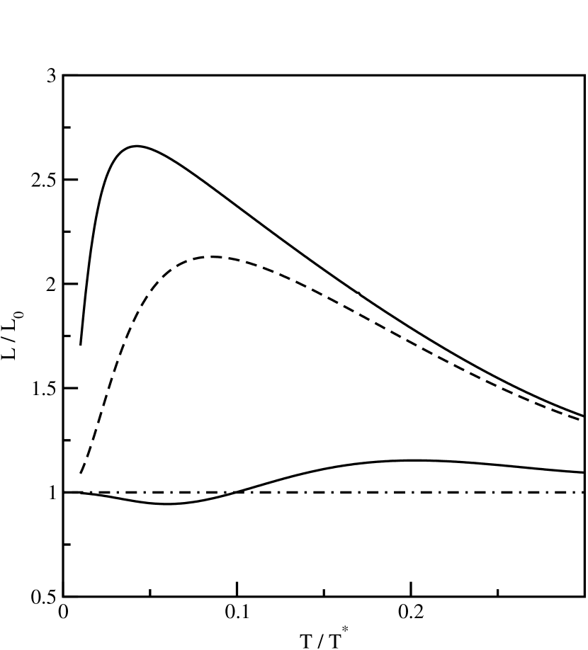
Refer to caption
Figure 1: The normalized Lorenz number as a function of temperature $(T)$. The dash-dotted curve is the result for the Born limit. Other curves are for the unitary limit. For the upper solid curve $\gamma_{U}/W_{0}=0.001$ and $\mu/W_{0}=-0.01$. The dashed curve is for the same chemical potential but for $\gamma_{U}/W_{0}=0.01$. The lower solid curve is for $\gamma_{U}/W_{0}=0.001$ but now $\mu/W_{0}=-0.15$.

It is not possible to obtain analytic results for the unitary limit. In general the Lorenz number $L(T)/L(0)$ is written as

$$\frac{L(T)}{L_{0}}=\frac{3}{\pi^{2}}\frac{\int d\omega\left(\frac{\omega}{T}\right)^{2}\left(-\frac{\partial f}{\partial\omega}\right){\cal A}(\omega)}{\int d\omega\left(-\frac{\partial f}{\partial\omega}\right){\cal A}(\omega)}\;.$$ (25)

As we mentioned earlier, in the unitary limit $\gamma(\omega)=\gamma_{U}\left(\frac{W_{0}}{\omega+\mu}\right)\ln^{-2}\left(\frac{W_{0}}{|\omega+\mu|}\right)$. Numerical results are presented in Fig.Β 1. We show results for four different cases which serve to illustrate what is possible. The upper solid curve is for $\gamma_{U}/W_{0}=0.001$ and $\mu/W_{0}=-0.01$ which shows a large peak around $T/T^{*}=0.05$. We have taken $T^{*}$ to be given by its mean field value: $W_{0}/T^{*}=2.14$ as in the DSC case. A very large positive violation of the WF law is seen. We need to point out, however, that while we have not shown $\sigma(T)$ and $\kappa(T)/T$ individually, in this case they both show large variations with $T$ reflecting the important frequency variation of $\gamma(\omega)$ for the unitary limit, which is not compensated for by the explicit variation of ${\cal A}(\omega)$ in Eq.(7). For the Born limit an exact compensation takes place so that ${\cal A}(\omega)$ turns out to be a constant. This leads to the usual WF law with no $T$ dependence, which is shown as a dash-dotted line in Fig.Β 1. For the dashed curve $\gamma_{U}/W_{0}=0.01$ and $\mu/W_{0}=-0.01$. Increasing $\gamma_{U}$ makes the deviations from the conventional Lorenz number smaller. The same effect is obtained when $|\mu|$ is increased, effectively pushing the FS further away from the zero in DOS. The second solid curve has $\gamma_{U}/W_{0}=0.001$ but now $\mu/W_{0}=-0.15$, away from half filling. Now the deviation from the conventional Lorenz number can be negative as well as positive depending on $T$ but the amplitude of the violation is small because the DDW gap becomes less effective at changing the DOS near the FS. (Note that $|\mu|\ll W_{0}$ for the validity of the nodal approximation.)

Our main conclusions are as follows. At $T=0$, only the zero frequency limit of the imaginary part of the self-energy enters into the calculation of the electrical and thermal conductivity and the conventional Wiedemann-Franz (WF) law is recovered. In contrast with what is found for a $d$-wave superconductor (DSC), for a $d$-density wave (DDW) state, neither electrical nor thermal conductivity show universal behavior. Each depends on the impurity scattering rate. But this dependence is the same and cancels from the Lorenz number as $T\rightarrow 0$. We were also able to obtain analytic results for low but finite temperature. In this case we found no change in the WF law for the Born limit even though the Lorenz number is reduced by a factor of two from its conventional value for the DSC. For the unitary limit, however, the Lorenz number increases rapidly at low temperature on a scale set by the zero scattering rate $\gamma(0)$. In a case considered it rises above $2.5$ around $T/T^{*}\simeq 0.05$ and then acquires a more moderate temperature variation. This case corresponds to the chemical potential $(\mu)$ small compared to the DDW gap. When $|\mu|$ is increased sufficiently, the Lorenz number becomes approximately equal to its conventional value and its temperature dependence is small. It is important to realized that when the Lorenz number is found to vary significantly with temperature, so do both electrical and thermal conductivities. This is generic to the model in which quasiparticles are responsible for the transport. Such a model cannot explain experimentshill in which the D.C. conductivity is almost independent of temperature while the Lorenz number is strongly dependent on it.

Acknowledgements.
This work was supported in part by the Natural Sciences and Engineering Research Council of Canada (NSERC) and by the Canadian Institute for Advanced Research (CIAR).

References

  • (1) R. W. Hill et al. , Nature (London) 414, 711 (2001).
  • (2) S. Chakravarty, R. B. Laughlin, D. Morr, and C. Nayak, Phys. Rev. B 63, 094503 (2001).
  • (3) S. Chakravarty, H. -Y. Kee, and C. Nayak, Int. J. Mod. Phys. B 15, 2901 (2001).
  • (4) Q. -H. Wang, J. H. Han, and D. -H. Lee, Phys. Rev. Lett. 87, 077004 (2001).
  • (5) J. -X. Zhu, W. Kim, C. S. Ting, and J. P. Carbotte, Phys. Rev. Lett. 87, 197001 (2001).
  • (6) W. Kim, J. -X. Zhu, J. P. Carbotte, and C. S. Ting, Phys. Rev. B 65, 064502 (2002).
  • (7) H. Ding et al. , Nature (London) 382, 51 (1996); A. G. Loeser et al. , Science 273, 325 (1996).
  • (8) A. C, Durst and P. A. Lee, Phys. Rev. B 62, 1270 (2000).
  • (9) P. J. Hirschfeld, P. WΓΆlfle, and D. Einzel, Phys. Rev. B 37, 83 (1988); P. J. Hirschfeld, W. O. Putikka, and D. J. Scalapino, Phys. Rev. B 50, 10250 (1994).
  • (10) M. J. Graf, S. -K. Yip, J. A. Sauls, and D. Rainer, Phys. Rev. B 53, 15147 (1996).