Segregation in hard sphere mixtures under gravity. An extension of Edwards approach with two thermodynamical parameters

Abstract

We study segregation patterns in a hard sphere binary model under gravity subject to sequences of taps. We discuss the appearance of the “Brazil nut” effect (where large particles move up) and the “reverse Brazil nut” effects in the stationary states reached by “tap” dynamics. In particular, we show that the stationary state depends only on two thermodynamical quantities: the gravitational energy of the first and of the second species and not on the sample history. To describe the properties of the system, we generalize Edwards’ approach by introducing a canonical distribution characterized by two configurational temperatures, conjugate to the energies of the two species. This is supported by Monte Carlo calculations showing that the average of several quantities over the tap dynamics and over such distribution coincide. The segregation problem can then be understood as an equilibrium statistical mechanics problem with two control parameters.

Segregation is an ubiquitous and intriguing phenomenon observed in vibrated granular mixtures such as powders or sand: in presence of shaking the system is not randomized, but its components tend to separate [1, 2]. An example is the so called “Brazil nut” effect (BNE) where, under shaking, large particles rise to the top and small particles move to the bottom of the container. Several mechanisms have been proposed to explain these phenomena, as for instance “percolation” [3], geometrical reorganization [4, 5], convection [6], “condensation” [7] or inertia [8]. Interestingly, by changing grains sizes or mass ratio a crossover towards a “reverse Brazil nut” effect (RBNE) was more recently discovered [7] where small particles segregates to the top and large particles to the bottom. On the whole the criteria to predict segregation in a mixture, an issue of large practical relevance, are still largely unknown [1].

In the perspective of the Statistical Mechanics approach originally proposed by Edwards to describe powders [9], we study here segregation patterns, in absence of convection mechanisms, of a binary hard sphere model under gravity subject to sequences of “taps”. We show that a Statistical Mechanics description of segregation is indeed possible by the introduction of two “configurational temperatures” which characterize the macroscopic status of the system.

In Edwards’ approach granular media at rest (i.e., when grains have no kinetic energy and, thus, the bath temperature is zero) can be described in terms of Statistical Mechanics where a single control parameter, called compactivity, plays the role of the temperature of usual thermal systems [9, 10, 11, 12, 13]. We show that the stationary states of the present mixture are indeed independent on the sample history as in a “thermodynamics” system, but are characterized by two control parameters, such as the gravitational energy of the first and of the second species. We postulate that the probability distribution of the system in the stationary state can be obtained by the principle of maximum entropy under the constraint that the two energies are independently fixed. This leads to a Gibbs canonical distribution characterized by two configurational temperatures, conjugate to the energies of the two species, generalizing in this way Edwards approach [15] . The postulate is supported by Monte Carlo simulations showing for several quantities that statistical averages over the tap dynamics coincide with those over such an ensemble distribution. The segregation problem can then be studied as standard Statistical Mechanics problems using such a distribution and, for instance, a segregation “phase” diagram can be theoretically derived.

We consider a binary hard sphere system made of two species 1 (small) and 2 (large) with grain diameters $a_{0}$ and $\sqrt{2}a_{0}$, under gravity on a cubic lattice of spacing $a_{0}=1$ (see inset of Fig.1). The hard core potential ${\cal H}_{hc}$ is such that two nearest neighbor particles cannot overlap. This implies that only pairs of small particles can be nearest neighbors on the lattice. The system overall Hamiltonian is:

$${\cal H}={\cal H}_{hc}+m_{1}gH_{1}+m_{2}gH_{2},$$ (1)

where $H_{1}=\sum_{i}^{(1)}z_{i}$ and $H_{2}=\sum_{i}^{(2)}z_{i}$, the height of site $i$ is $z_{i}$ and the two sums are over all particles of species 1 and 2 respectively. We set the units such that the two kinds of grain have masses $m_{1}=1$ and $m_{2}=2$, and the gravity acceleration is $g=1$. In the above units, the gravitational energies in a given configuration are thus $E_{1}=H_{1}$ and $E_{2}=2H_{2}$.

Grains are confined in a box of linear size $L$ between hard walls and periodic boundary conditions in the horizontal directions. The system is subject to a Monte Carlo dynamics made of sequences of “taps” [16, 10, 11]. During each “tap” the system evolves for a time $\tau_{0}$ (the “tap duration”, in units of lattice sweeps) in presence of a finite thermal bath of temperature $T_{\Gamma}$; afterwards it is suddenly frozen at zero temperature in one of its stable states. These states correspond to a local minimum or saddle of the energy, such that any particle movement does not decrease the energy, and have been called “inherent states” [11] in analogy with the terminology of glasses [17]. After each tap, when the system is at rest, we record the quantity of interest, which are a function of the number of “taps”, $t$.

$N_{1}$ grains of type 1 and $N_{2}$ grains of type 2 are initially prepared in a random loose stable pack [18]. Under “shaking” the system is let to approach a stationary state for each value of the tap parameters $T_{\Gamma}$ and $\tau_{0}$, as shown in Fig.1 for the large grains height $h_{2}(t)=H_{2}(t)/N_{2}$. In Fig.2, we plot as function of $T_{\Gamma}$ (for several values of $\tau_{0}$) the asymptotic value of the vertical segregation parameter, i.e., the difference of the average heights of the small and large grains at stationarity, $\Delta h(T_{\Gamma},\tau_{0})\equiv h_{1}-h_{2}$. Here $h_{1}$ and $h_{2}$ are the average of $H_{1}/N_{1}$ and $H_{2}/N_{2}$ over the tap dynamics in the stationary state.

Fig.2 shows that at high $T_{\Gamma}$ the Brazil Nut Effect (BNE) of granular media is observed: “large” grains are found on the top of the system (i.e., $\Delta h<0$). For small values of $T_{\Gamma}$, below a crossover amplitude, $T^{*}_{\Gamma}(\tau_{0})$, a smooth crossover to the Reverse Brazil Nut Effect (RBNE) is instead recorded, with $\Delta h>0$. The RBNE was first discovered in recent Molecular Dynamics simulations [7]. Our aim below is to show that the properties of these segregation patterns can be explained in terms of a statistical mechanics approach to the problem.

The results given in the main panel of Fig. 2 apparently show that $T_{\Gamma}$ is not a right “thermodynamical” parameter, since sequences of “taps” with different $\tau_{0}$ give different values for the system observables. However, if the stationary states corresponding to different tap dynamics (i.e., different $T_{\Gamma}$ and $\tau_{0}$), are indeed characterized by a single “thermodynamical” parameter á la Edwards, the curves of Fig.2 should collapse on an universal master function when $\Delta h(T_{\Gamma},\tau_{0})$ is parametrically plotted as function of an other macroscopic observable such as the average energy, $e(T_{\Gamma},\tau_{0})=(E_{1}+E_{2})/N={N_{1}\over N}h_{1}+{2N_{2}\over N}h_{2}$ (where $N=N_{1}+N_{2}$). This collapse of data, actually found in other situations [10, 11], is clearly not observed here, as it is apparent in the inset of Fig.2 (see also [14]).

We show, instead, that two macroscopic quantities, such as $h_{1}$ and $h_{2}$, may be sufficient to characterize uniquely the stationary state of the system. Namely, we show that any macroscopic quantity $Q$, averaged over the tap dynamics in the stationary state, is only dependent on $h_{1}$ and $h_{2}$, i.e., $Q=Q(h_{1},h_{2})$. We have checked that this is the case for several independent observables, such as the number of contacts between large particles, $N_{c}$, the density of small and large particles on the bottom layer, $\rho_{1}^{b}$ and $\rho_{2}^{b}$, and others. As shown in Fig.3, we find, in particular, with good approximation that: $N_{c}\simeq N_{c}(e)=N_{c}({N_{1}\over N}h_{1}+{2N_{2}\over N}h_{2})$, $\rho_{2}^{b}\simeq\rho_{2}^{b}(h_{2})$, $\rho_{1}^{b}\simeq\rho_{1}^{b}(h_{1})$. Therefore we need both $h_{1}$ and $h_{2}$ (or equivalently $E_{1}$ and $E_{2}$) to characterize unambiguously the state of the system independently on the previous history (i.e., in our case independently on the particular tapping parameters $T_{\Gamma}$ and $\tau_{0}$).

In this respect the stationary state can be genuinely considered as a “thermodynamical state”, and consequently one can attempt to construct an equilibrium statistical mechanics, as originally suggested by Edwards. This will allow to calculate any quantity in the stationary state using an appropriate ensemble, irrespective of the particular history.

In the present paper we generalize Edwards’ approach by introducing a canonical distribution characterized by two configurational temperatures, conjugate to the energies of the two species, and verify by Monte Carlo calculations that the average of several quantities over the tap dynamics and over such distribution coincide. More precisely we have to find the probability distribution, $P_{r}$, of observing the system in the generic inherent state $r$ corresponding to an energy $E_{1r}$ for the small particles and $E_{2r}$ for the large particles (see [11]). To answer this, we assume that the microscopic distribution is given by the principle of maximum entropy $S=-\sum_{r}P_{r}\ln P_{r}$ under the condition that the average energy $E_{1}=\sum_{r}P_{r}E_{1r}$ and $E_{2}=\sum_{r}P_{r}E_{2r}$ are independently fixed. This can be done by introducing two Lagrange multipliers $\beta_{1}$ and $\beta_{2}$, which are determined by the constraint on $E_{1}$ and $E_{2}$, and can be considered as the “inverse configurational temperature” of species 1 and 2 [11]. This procedure leads to the Gibbs result:

$$P_{r}=\frac{e^{-\beta_{1}E_{1r}-\beta_{2}E_{2r}}}{Z}$$ (2)

where $Z=\sum_{r}\exp\left[-\beta_{1}E_{1r}-\beta_{2}E_{2r}\right]$ and, in the thermodynamic limit, the entropy, $S$, is given by:

$$S=\ln\Omega(E_{1},E_{2}),$$ (3)

and $\beta_{1}$ and $\beta_{2}$:

$$\beta_{1}=\frac{\partial\ln\Omega(E_{1},E_{2})}{\partial E_{1}},\quad\beta_{2}=\frac{\partial\ln\Omega(E_{1},E_{2})}{\partial E_{2}}.$$ (4)

Here $\Omega(E_{1},E_{2})$ is the number of inherent states corresponding to energy $E_{1}$ and $E_{2}$.

The hypothesis that the ensemble distribution at stationarity is given by eq.(2) can be tested as follows. We have to check that the time average of any quantity, $Q(h_{1},h_{2})$, as recorded during the taps sequences in a stationary state characterized by given values $h_{1}$ and $h_{2}$, must coincide with the ensemble average, $\langle Q\rangle(h_{1},h_{2})$, over the distribution eq.(2). To this aim, we have calculated the ensemble averages $\langle N_{c}\rangle$, $\langle\rho_{2}^{b}\rangle$, $\langle\rho_{1}^{b}\rangle$, for different values of $\beta_{1}$ and $\beta_{2}$; then we have expressed parametrically $\langle N_{c}\rangle$, $\langle\rho_{2}^{b}\rangle$, $\langle\rho_{1}^{b}\rangle$, as function of the average of $h_{1}$ and $h_{2}$, and compared them with the corresponding quantities, $N_{c}$, $\rho_{1}^{b}$ and $\rho_{2}^{b}$, averaged over the tap dynamics. The two sets of data are plotted in Fig.3 showing a rather good agreement (notice, there are no adjustable parameters). Technically, in order to calculate the ensemble averages we simulated, with standard Monte Carlo methods, the model with $\cal H$ from eq.(1) where we impose that the only accessible states are the inherent states. This can be done by using a configurational Hamiltonian

$${\cal H}_{conf}={\cal H}_{hc}+\beta_{1}m_{1}gH_{1}+\beta_{2}m_{2}gH_{2}-\ln\Pi,$$ (5)

where $\Pi=1$ or $0$ depending whether the configuration is an inherent state or not. In this way the weight $e^{-{\cal H}_{conf}}$ gives the ensamble distribution (2) (for further details see [11, 13]). The discovery of two configurational temperatures may suggest the existence of more than one “dynamical temperature” in the off-equilibrium fluctuation-dissipation relation approach of [13, 19].

We show now how the ensemble averages with the distribution (2) can be analytically calculated for a simple toy model of a mixture of two particles. The model can be visualized as a cell of the above hard sphere pack, made of one large and two small grains seating on the vertices of a square lattice, with three layers each of 2 sites. Interestingly, such a three levels system is able to reproduce the general properties found before. In particular, the resulting diagram for segregation is plotted in Fig.4 in the plane $T_{1}=(m_{1}ga_{0}\beta_{1})^{-1}$, $T_{2}=(m_{2}ga_{0}\beta_{2})^{-1}$. It shows that for a given value of $T_{1}$ by decreasing $T_{2}$ the system undergoes a crossover, at $T_{2}^{*}(T_{1})$, from a region where type-2 particles are on average above (BNE) to a region where they are below (RBNE) type-1 particles. The structure of the diagram of Fig.4, for small values of $T_{1}$ and $T_{2}$, can be easily understood by looking at eq.(2): when the configurational temperature of small particles, $T_{1}$, is much smaller than the other, $T_{2}$, the potential energy of small grains is much smaller than that associated to the large ones, therefore large grains segregate on top (BNE). The opposite happens when $T_{2}$ is close to zero and much smaller than $T_{1}$. In particular, in this toy model the RBNE region cannot be met if $T_{2}$ is too large.

The crossover observed in vertical segregation from BNE to RBNE corresponds to the drift of the minimum of the free energy, $F=-\ln Z$, from negative to positive values of $\Delta h$. In this scenario, the pack undergoing a taps dynamics with “amplitudes” $T_{\Gamma}$ (and given “duration”, $\tau_{0}$) at stationarity, as for the data shown in Fig.2, can be thus thought to be following a given path, $T_{2}=T_{2}(T_{1})$ (where $T_{1}=T_{1}(T_{\Gamma},\tau_{0})$), in the $(T_{1},T_{2})$ plane, crossing from the BNE to the RBNE region.

In conclusion, we have shown that in the present hard sphere binary mixture model Edwards’ approach to describe segregation holds if two thermodynamical parameters are introduced. In the case considered here these two thermodynamical parameters play the role of configurational temperatures related to the two types of particles. By applying all the standard techniques of statistical mechanics of the canonical distribution one can thus predict the complex segregation patterns as found above. In particular we have shown on a hard sphere mixture on a lattice that the segregation phenomena in granular media can be studied applying standard statistical mechanics to a new Hamiltonian (5), which contains the original Hamiltonian of the grains plus a term which constrains the system to be in a inherent state.

In general for a more complex system one might expect more constraints to be imposed, leading to more than two thermodynamical parameters. In practice, the criteria to determine a priori the required parameters can be not easily accessible. However more recently we have extended data for very low energy [20] and found that only one thermodynamical parameter is necessary to describe the stationary state. This seems to be a general feature [11]. If this is the case, a Statistical Mechanics approach with only one thermodynamical variable may be feasible for low energy.

This work was partially supported by the TMR-ERBFMRXCT980183, INFM-PRA(HOP), MURST-PRIN 2000 and MURST-FIRB 2002. The allocation of computer resources from INFM Progetto Calcolo Parallelo is acknowledged.

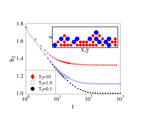
FIG. 1.: Main frame The relaxation of large grains average height, $h_{2}$, as a function of the number of taps, $t$, in taps sequences with the shown shaking amplitudes, $T_{\Gamma}$ (tap duration, $\tau_{0}=10$). The superimposed curves are stretched exponential fits. Inset A schematic picture of the 3D lattice hard sphere mixture considered here.

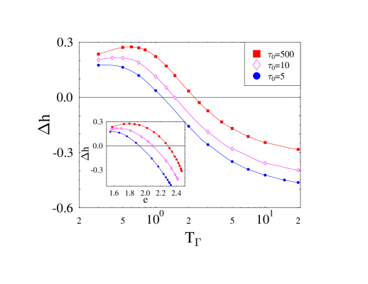
FIG. 2.: Main frame The difference of the average heights of small and large grains, $\Delta h=h_{1}-h_{2}$, measured at stationarity is plotted as a function of tap amplitude, $T_{\Gamma}$. The three sets of points correspond to the shown tap durations, $\tau_{0}$. At high $T_{\Gamma}$ larger grains are found above the smaller, i.e, $\Delta h<0$, as in the Brazil nut effect (BNE). Below a $T^{*}_{\Gamma}(\tau_{0})$ the opposite is found (Reverse Brazil nut effect, RBNE). Inset The $\Delta h$ data of the main frame are plotted as a function of the corresponding average energy, $e$. The three sets of data do not collapse on a single master function, showing that a single macroscopic observable, such as $e$, doesn’t characterize unambiguously the system status.

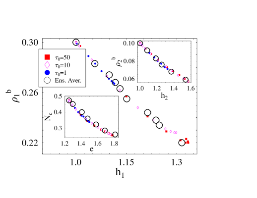
FIG. 3.: Main frame The average density of small grains on the box bottom layer, $\rho_{1}^{b}$, measured at stationarity as a function of the height of small particles, $h_{1}$. Data corresponding to different $T_{\Gamma}$ and $\tau_{0}$ approximately scale on a single master function. The empty circles are the corresponding values obtained by ensemble average with the two temperatures Gibbs measure proposed in the text. Upper inset The average density of large grains on the box bottom layer, $\rho_{2}^{b}$, obtained for different $T_{\Gamma}$ and $\tau_{0}$, scale almost on a single master function when plotted as a function of the large grains height, $h_{2}$. Lower inset The average number of contacts between large grains per particle, $N_{c}$, obtained for different $T_{\Gamma}$ and $\tau_{0}$, scale on a single master function when plotted as a function of the system energy, $e$.

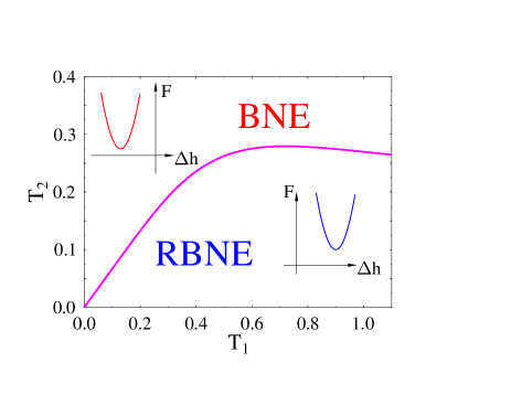
FIG. 4.: The analytically calculated diagram for segregation in the plane $T_{1}=(m_{1}ga_{0}\beta_{1})^{-1}$, $T_{2}=(m_{2}ga_{0}\beta_{2})^{-1}$ in the three levels model described in the text ($\beta_{i}$ is the inverse configurational temperature of the grains of type $i$). The crossover from Brazil nut effect (BNE) to reverse Brazil nut effect (RBNE) corresponds to the drift of the minimum of the free energy in the inherent states space, $F$, from negative to positive values of the vertical segregation parameter, $\Delta h$.

REFERENCES

- [1] J.M. Ottino and D.V. Khakhar, Ann. Rev. Fluid Mech. 32, 55 (2000). H.M. Jaeger, S.R. Nagel and R.P. Behringer, Rev. Mod. Phys. 68, 1259 (1996). J. Bridgewater, Chem. Eng. Sci. 50, 4081 (1995).
- [2] H.A. Makse, S. Havlin, P.R. King, and H.E. Stanley, Nature 386, 379 (1997). T. Shinbrot, A. Alexander, F.J. Muzzio, Nature 397, 675 (1999). M.E. Möbius, B.E. Lauderdale, S.R. Nagel, H.M. Jaeger, Nature 414, 270 (2001).
- [3] T. Rosato, F. Prinze, K.J. Standburg, R. Swendsen, Phys. Rev. Lett. 58, 1038 (1987).
- [4] J. Bridgewater, Powder Technol. 15, 215 (1976). J.C. Williams, Powder Technol. 15, 245 (1976).
- [5] J. Duran, J. Rajchenbach, E. Clement, Phys. Rev. Lett. 70, 2431 (1993).
- [6] J. Knight, H. Jaeger, S. Nagel, Phys. Rev. Lett. 70, 3728 (1993).
- [7] D.C. Hong, P.V. Quinn, S. Luding, Phys. Rev. Lett. 86, 3423 (2001). J.A. Both and D.C. Hong, Phys. Rev. Lett. 88, 124301 (2002).
- [8] T. Shinbrot and F. Muzzio, Phys. Rev. Lett. 81, 4365 (1998).
- [9] S.F. Edwards and R.B.S. Oakeshott, Physica A 157, 1080 (1989). A. Mehta and S.F. Edwards, Physica A 157, 1091 (1989). S.F. Edwards, in Current Trends in the physics of Materials, (Italian Phys. Soc., North Holland, Amsterdam, 1990).
- [10] A. Lefèvre, D. S. Dean, Phys. Rev. Lett. 86, 5639 (2001).
- [11] A. Coniglio and M. Nicodemi, Physica A 296, 451 (2001). A. Fierro, M. Nicodemi and A. Coniglio, Europhys. Lett. 59 (5), 642 (2002).
- [12] J.J. Brey, A. Prados, B. Sánchez-Rey, Physica A 275, 310 (2000).
- [13] A. Barrat, J. Kurchan, V. Loreto and M. Sellitto, Phys. Rev. Lett. 85, 5034 (2000). H.A. Makse and J. Kurchan, Nature 415, 614 (2002).
- [14] J. Berg, S. Franz and M. Sellitto, Eur. Phys. J. B 26, 349 (2002).
- [15] The possibility of introducing more than one thermodynamical parameter has been also suggested in [14] and very recently discussed in the context of a Constrained Ising Chain by A. Lefèvre, cond-mat/0202376.
- [16] M. Nicodemi, A. Coniglio, H.J. Herrmann, Phys. Rev. E 55, 3962 (1997). A. Coniglio, M. Nicodemi, J. Phys.: Cond. Matt. 12, 6601 (2000). M. Nicodemi, Physica A 285, 267 (2000).
- [17] F.H. Stillinger T.A. Weber, Phys. Rev. A 25, 978 (1982). S. Sastry, P.G. Debenedetti, F.H. Stillinger, Nature 393, 554 (1998). B. Coluzzi, G. Parisi and P. Verrocchio, Phys. Rev. Lett. 84, 306 (2000). F. Sciortino, W. Kob, P. Tartaglia, Phys. Rev. Lett. 83, 3214 (1999). F. Sciortino and P. Tartaglia, Phys. Rev. Lett. 86, 107 (2001).
- [18] We considered two kinds of systems: a box of size , with small and large grains; and a box of size , with and . Our data are averaged on up to 16384 realizations. We also considered sizes up to 32, up to 480 and up to 160.
- [19] M. Nicodemi, Phys. Rev. Lett. 82, 3734 (1999).
- [20] A. Coniglio, A. Fierro, M. Nicodemi, in preparation.