A Role of Initial Conditions in
Spin-Glass Aging Experiments

Abstract

Effect of initial conditions on aging properties of the spin-glass state is studied for a single crystal Cu:Mn 1.5 at %. It is shown that memory of the initial state, created by the cooling process, remains strong on all experimental time scales. Scaling properties of two relaxation functions, the TRM and the IRM (with $t_{w1}=0$ and $t_{w2}=t_{w}$), are compared in detail. The TRM decay exhibits the well-known subaging behavior, with $\mu<1$ and $t_{w}^{e\!f\!f}>t_{w}$. The IRM relaxation demonstrates the superaging behavior, with $\mu>1$ and $t_{w}^{e\!f\!f}<t_{w}$. It is shown that an average over different initial conditions leads to systematic improvement in $t/t_{w}$ scaling. An effective barrier, describing influence of the initial state on spin-glass relaxation, is found to be almost independent of temperature. These results suggest that departures from full $t/t_{w}$ scaling, observed in aging experiments, are largely due to cooling effects.

I Introduction

Aging phenomena in spin glasses have been studied for almost twenty years.lun83 Despite considerable progress, some problems remain open. One of them is a problem of $t/t_{w}$ scaling of time dependent quantities.vin96 This issue is a touchstone of our understanding of spin-glass dynamics. Only when all departures from full $t/t_{w}$ scaling are accounted for, both theoretically and experimentally, can one say that the aging phenomena are well understood.

First experimental results on $t/t_{w}$ scaling of the thermoremanent magnetization (TRM) were obtained soon after the aging effects had been discovered. They demonstrated that there are small but systematic deviations from full $t/t_{w}$ scaling in the aging regime.oci85 ; alb87 It was shown that the TRM curves for different waiting times can be successfully superimposed if a power of the waiting time, $t_{w}^{\mu}$, with $\mu<1$, is used in the analysis instead of the actual $t_{w}$. This phenomenon is often referred to as “subaging”. The apparent age of the spin-glass state, determined from the scaling of the TRM curves, increases slower than the waiting time $t_{w}$. It was also shown oci85 ; alb87 that the quasiequilibrium decay at short observation times should be taken into account properly in order to achieve good scaling over a wide time range. However, full $t/t_{w}$ scaling in the aging regime has never been derived from experimental data. Deviations of $\mu$ from unity are small, but persistent. The physical meaning of this scaling parameter remains unclear even though different interpretations have been proposed.bou94 ; rin00 All this suggests that there may be some additional reasons for the lack of scaling, which have not been taken into account yet.

On the theoretical side, the situation is more ambiguous. Phenomenological phase-space models,bou92 ; bou95 describing aging as thermally activated hopping over free-energy barriers, suggest full $t/t_{w}$ scaling in the absence of finite-size effects. In the mean-field dynamics, however, two different cases are distinguished.bou97 Those mean-field models, where one level of replica-symmetry breaking is exact (like the spherical $p$-spin model), have only one time scale in the aging regime, and $t/t_{w}$ scaling is predicted.cug93 Models with continuous replica-symmetry breaking (like the Sherrington-Kirkpatrick model), are characterized by an infinite number of time scales.cug94 If decay of the correlation function in the aging regime is viewed as a sequence of infinitesimal steps, then each step takes much longer than the previous one.cug99 Therefore, no $t/t_{w}$ scaling is expected in these models. It is suggestedbou97 ; cug99 that full $t/t_{w}$ scaling for all times in the aging regime would rule out the continuous replica-symmetry breaking scenario. Thus, a reliable experimental evidence of presence (or absence) of $t/t_{w}$ scaling may help determine validity of different theoretical pictures.

Numerical studies of spin-glass dynamics reveal an interesting fact. The short-range 3-dimensional Edwards-Anderson (EA) model exhibits good $t/t_{w}$ scaling,kis96 ; rit01 while there is no such scaling in the infinite-range Sherrington-Kirkpatrick (SK) model.mar98 ; tak97 ; rit94 However, validity of the EA model for description of real spin-glasses has been questioned. Recent simulations pic01 have shown no trace of rejuvenation effects, observed in temperature-change experiments.jon00 It was argued that either time scales, reached in simulations, are too short, or the Edwards-Anderson model is not a good model for real spin glasses.pic01 Further studies of both $t/t_{w}$ scaling and temperature-variation effects are needed to find out which model is better suited for theoretical description of spin-glass dynamics.

The present paper is devoted to a study of departures from full $t/t_{w}$ scaling in spin-glass aging experiments. We hypothesize that one of possible reasons for the lack of such scaling is the influence of the cooling process. Our line of argument is the following. A typical spin-glass relaxation experiment includes cooling from above the glass temperature.nor87 Approach of the measurement temperature is necessarily slow with possible oscillations, because temperature has to be stabilized. Temperature-cycling experiments,ref87 ; led91 ; ham92 as well as aging experiments with different cooling rates,nor00 have shown that thermal history near the measurement temperature has a profound effect on the subsequent spin-glass behavior. Any aging experiment is, therefore, a temperature-variation experiment, and measured relaxation properties are determined by both cooling and waiting time effects. As the waiting time increases, the influence of the initial condition, set by the cooling process, diminishes. This may lead to a systematic deviation from full $t/t_{w}$ scaling, compatible with the experimentally observable behavior. In order to extract relaxation curves that exhibit good $t/t_{w}$ scaling, one has to average experimental results over different initial conditions.

The paper is organized as follows. The next Section discusses general properties of spin-glass relaxation and methods for analysis of $t/t_{w}$ scaling. In Sec. III.A, features of the cooling process and properties of the TRM decay for $t_{w}=0$ are studied. Sec. III.B discusses two different types of deviations from $t/t_{w}$ scaling. In Sec. III.C, properties of the TRM and the IRM are analyzed in detail. The effect of initial conditions on scaling properties of measured relaxation is discussed in Sec. III.D. The last Section summarizes our arguments.

II Theoretical background

II.1 Linear response in spin glasses

In a typical TRM experiment, a spin-glass sample is cooled down from above the glass temperature $T_{g}$ to a measurement temperature $T<T_{g}$ in the presence of a small magnetic field $h$. It is then kept at the measurement temperature for some time $t_{w}$, which is called waiting time. After that, the field $h$ is cut to zero, and a decay of the thermoremanent magnetization (TRM) is measured as a function of observation time $t$, elapsed after the field change. This decay depends on the waiting time $t_{w}$ – a phenomenon called aging. The total age of the system is $t+t_{w}$. In a more complex IRM protocol, the sample is cooled down at zero magnetic field and kept for a waiting time $t_{w1}$. Then a small magnetic field is turned on, and, after an additional waiting time $t_{w2}$, is turned off again. A subsequent decay of the isothermal remanent magnetization (IRM) is observed. It depends on both waiting times.

In order to describe time evolution of the system, the autocorrelation function, $C(t_{1},t_{2})$, is introduced:

$$C(t_{1},t_{2})=(1/N)\sum_{i=1}^{N}\langle S_{i}(t_{1})S_{i}(t_{2})\rangle~{}~{}.$$ (1)

It depends on two times, $t_{1}$ and $t_{2}$, measured from the end of the cooling process. Response of the system at time $t_{1}$ to an instantaneous field $h$, present at time $t_{2}$, is described by the response function:

$$R(t_{1},t_{2})=(1/N)\sum_{i=1}^{N}\delta\langle S_{i}(t_{1})\rangle/\delta h(t_{2})~{}~{}.$$ (2)

In thermal equilibrium, both functions depend only on the time difference, $t_{1}-t_{2}$, and they are related by the fluctuation-dissipation theorem. If the system is out of equilibrium, a generalization of this theorem is expected to hold:bou97

$$R(t_{1},t_{2})=\beta X[C]\,\partial C(t_{1},t_{2})/\partial t_{2}~{}~{}.$$ (3)

Here $\beta=1/k_{B}T$, and $X[C]$ is the fluctuation-dissipation ratio, which is equal to unity in equilibrium. It is suggested bou97 that, for long waiting times, $X$ depends on its time arguments only through the correlation function, i.e. $X(t_{1},t_{2})=X[C(t_{1},t_{2})]$.

Magnetic susceptibility, measured in spin-glass experiments, is the integrated response. If the field is present during the waiting time, $t_{w}$, the susceptibility, measured at the observation time, $t$, is given by the following expression:

$$\chi(t+t_{w},t_{w})=\int_{0}^{t_{w}}R(t+t_{w},t^{\prime})dt^{\prime}~{}~{}.$$ (4)

Using Eq. (3) for the response function and introducing a function $Y[C]$ through a relation $\beta X[C]=dY/dC$,bou95 one obtains the formula:

$$\chi(t+t_{w},t_{w})=Y[C(t+t_{w},t_{w})]-Y[C(t+t_{w},0)]~{}~{}.$$ (5)

The first term on the right is identified with the $t_{w}$-dependent TRM susceptibility.bou95 The second term corresponds to the TRM decay after zero waiting time. To avoid confusion, we shall refer to it as ZTRM, and drop the second argument. The function on the left is the IRM susceptibility for $t_{w1}=0$ and $t_{w2}=t_{w}$. In what follows, the IRM will always denote the isothermal remanent magnetization with $t_{w1}=0$. It is characterized by the same waiting time, $t_{w}$, as the TRM. We shall also use a corresponding observation time instead of a total age as the first argument of each function. For the ZTRM, the total age is equal to the observation time. Thus, Eq. (5) can be rewritten in the following form:

$$\chi_{IRM}(t,t_{w})=\chi_{TRM}(t,t_{w})-\chi_{ZTRM}(t+t_{w})~{}~{}.$$ (6)

The last formula expresses the well-known principle of superposition, which has been verified experimentally in the case of spin glasses.lun86

It follows from Eq. (6) that the TRM relaxation is a superposition of two decays. The IRM is a response, associated with the waiting time. The ZTRM is a response, related to the cooling process. However, the ZTRM itself cannot be treated as a linear response because of the changing temperature. This means that the thermal history cannot be taken into account by simple addition of the cooling time to the waiting time.

If memory of the initial state is strong, there will be no one-to-one correspondence between the $t_{w}$-dependent correlation and $t_{w}$-dependent linear response. The TRM depends on the correlation $C(t+t_{w},t_{w})$, but it includes response of the initial state. The IRM is a linear response, associated with the waiting time only, but it depends on the correlation with the initial state. Therefore, neither the TRM, nor the IRM can be called the ”true” $t_{w}$-dependent response.

The mean-field theory of aging phenomena relies on the assumption of weak long-term memory. According to this assumption, the system responds to its past in an averaged way, and its memory of any finite time interval in the past is weak.cug94 This implies that the lower integration limit, $t^{\prime}=0$, in Eq. (4) can be replaced by any finite $t^{\prime}=t_{0}$, as long as both $t$ and $t_{w}$ go to infinity.cug94 Thus, there should be no difference between the TRM and the IRM in the long-time limit. Within this asymptotic approach, the IRM is sometimes referred to as TRM. cug99 ; rit94

The linear response theory predicts that the measured susceptibility, Eq. (4), depends on the waiting time $t_{w}$. However, it gives no predictions regarding $t/t_{w}$ scaling. Eq. (6) suggests that the TRM and the IRM, though characterized by the same waiting time, cannot have the same scaling properties. This is because they differ by the ZTRM, which is a one-time quantity without a characteristic time scale. Two exceptional cases are possible. First, the ZTRM decays so rapidly, that the last term in Eq. (6) can be neglected for sufficiently large $t_{w}$. This case is usually considered in theoretical studies,vin96 ; bou95 which assume that memory of the initial condition is lost after very long waiting times, i.e. $C(t+t_{w},0)\rightarrow 0$ as $t_{w}\rightarrow\infty$.fra95 Second, the ZTRM changes so slowly, that $\chi_{ZTRM}(t+t_{w})$ for long enough $t_{w}$ can be treated as a non-zero constant. This approach is similar to the treatment of the field-cooled susceptibility, which is also a one-time quantity. We show in Sec. III.B that neither of these two conditions holds in spin-glass experiments.

II.2 Analysis of $t/t_{w}$ scaling

Spin-glass dynamics is characterized by at least two time scales. The microscopic attempt time, $\tau_{0}$, is associated with the quasiequilibrium decay at short observation times. The waiting time, $t_{w}$, determines properties of the nonequilibrium relaxation at long times. Both types of spin-glass behavior have to be taken into account when $t/t_{w}$ scaling of relaxation curves is analyzed.

Numerical studies of the off-equilibrium dynamics in the 3D Edwards-Anderson modelkis96 suggest that the autocorrelation function, $C(t,t_{w})$, can be well approximated by a product of two functions:

$$C(t,t_{w})\propto t^{-\alpha}\Phi(t/\,t_{w})~{}~{}.$$ (7)

The waiting time independent factor $t^{-\alpha}$ represents the slow (on the logarithmic scale) quasiequilibrium decay at $t\ll t_{w}$. The function $\Phi(t/t_{w})$ (which is approximately constant for $t\ll t_{w}$) describes the faster nonequilibrium relaxation at longer observation times. Of course, both $\alpha$ and $\Phi(x)$ depend on temperature.

A similar multiplicative ansatz comment has been successfully used for scaling experimental relaxation curves: oci85 ; alb87

$$\chi_{TRM}(t,t_{w})\propto t^{-\alpha}F(t_{e}/\,t_{w}^{\,\mu})~{}~{}.$$ (8)

Two features distinguish Eq. (8) from Eq. (7). First, an effective time $t_{e}$ (usually denoted by $\lambda$) is introduced. The age of the system increases with the observation time as $t_{w}+t$, and the time/age ratio decreases. In order to allow description of the relaxation by the same age $t_{w}$, the effective time should increase slower than the observation time $t$. This means that $dt_{e}/t_{w}=dt/(t+t_{w})$ and $t_{e}=t_{w}\ln(1+t/t_{w})$. Second, possible deviations from full $t/t_{w}$ scaling in the aging regime are taken into account by the parameter $\mu$. In this case, $dt_{e}/t_{w}^{\,\mu}=dt/(t+t_{w})^{\mu}$, and the effective time is

$$t_{e}=t_{w}[(1+t/t_{w})^{1-\mu}-1]/(1-\mu)~{}~{}.$$ (9)

At short observation times, $t\ll t_{w}$, the effective time is equivalent to the observation time: $t_{e}\approx t$.

The $\mu$-scaling approach is very useful for studying departures from $t/t_{w}$ scaling, no matter whether $\mu$ itself has a clear physical meaning or not. We use this method in the present paper and determine $\mu$ from juxtaposition of relaxation curves, plotted versus $t_{e}/t_{w}^{\,\mu}$.

A different method for separating the quasiequilibrium and aging regimes has also been successfully employed.vin96 It is inspired by dynamical solution of mean-field models. bou97 ; cug93 ; cug94 The following additive representation is considered: vin96

$$\chi_{TRM}(t,t_{w})\propto A(t/\tau_{0})^{-\alpha}+f(t_{e}/\,t_{w}^{\,\mu})~{}~{}.$$ (10)

This approach yields better $t/t_{w}$ scaling ($\mu$ closer to unity) than the previously discussed method. oci85 ; alb87 It should be noted, however, that derivation of the last formulavin96 employs an assumption that $C(t+t_{w},0)=0$. Therefore, Eq. (10) is exact only asymptotically (large $t_{w}$), when long-term memory is weak. Nevertheless, this method is justified, because it gives good results on experimental time scales.

III Experimental results and analysis

The purpose of this paper is to study how different initial conditions affect aging phenomena in spin-glass experiments. By the initial condition we mean history of the spin-glass state before the waiting time begins. We do not attempt to prove existence or absence of full $t/t_{w}$ scaling. We try to understand, on the qualitative level, where observable departures from the full scaling in the aging regime come from.

All experiments were performed on a single crystal of Cu:Mn 1.5 at %, a typical Heisenberg spin glass with a glass temperature of about $15.2~{}K$. The single crystal was used to avoid possible complications due to finite-size effects. Another advantage of this sample is its high de Almeida-Thouless (AT) critical line. zot01 For example, the AT field at $T/T_{g}=0.87$, the highest measurement temperature in our experiments, is about $600~{}Oe$. This enables us to use a relatively large field change, $\Delta H=10~{}Oe$, and still work well within the linear response regime. A commercial Quantum Design SQUID magnetometer was used for all the measurements. This equipment has been optimized for precision and reproducibility, rather than speed. Thus, cooling is relatively slow, and this allows us to study cooling effects in detail.

III.1 Cooling process and ZTRM

Spin-glass behavior is characterized by memory effects: properties of measured spin-glass relaxation depend on history of a sample below $T_{g}$. The cooling process is an integral part of this history. It has been shown that, in real spin glasses, details of the experimental protocol well above the measurement temperature, $T$, do not affect the measured relaxation.ref87 However, the thermal history in the immediate vicinity of the measurement temperature (say, $\delta T<0.5~{}K$) has a strong impact on the observed spin-glass behavior. This fact suggests that the cooling and waiting time effects cannot be separated and should be studied simultaneously.

A typical cooling protocol is exhibited in the inset of Fig. 1. The temperature drops rapidly to well below the measurement temperature, than rises to $T+\delta T$, and slowly approaches $T$ from above. By definition, the experimental time starts when the measurement temperature, $T$, is finally reached.

The approach of the measurement temperature is shown in the main body of Fig. 1. For relatively high temperatures, $\delta T\approx 0.1~{}K$. For the lowest temperature, however, $\delta T\approx 0.3~{}K$. Comparison with results of temperature-cycling experimentsref87 suggests that the initial undercool is not very important, because of its large (several Kelvin) magnitude. The subsequent overshoot, however, may be expected to play a significant role in spin-glass dynamics, and cannot be neglected in our experiments. It should be noted that Fig. 1 exhibits the temperature curves for helium gas, used as a heat transfer agent within a sample chamber. The actual temperature of the spin-glass sample lags behind. This means that, in reality, the undercool is probably less pronounced, and the sample spends more time above the measurement temperature.

Figure 1: Approach of the measurement temperature, $T$, during the cooling process. The temperature curves $T^{\prime}(t)$, from top to bottom, are for $T/T_{g}=0.3,0.4$, and $0.77$, respectively. The inset shows the whole cooling process for $T/T_{g}=0.77$.

It is instructive to compare the cooling procedure in Fig. 1 with an experimental protocol including a positive temperature cycle.ref87 In this protocol, the sample is field-cooled to the measurement temperature, $T$, and kept for a long waiting time $t_{w1}$. Then it is heated up to $T+\delta T$ and annealed for a short time $t_{w2}$. After that, it is cooled down and kept at the initial temperature $T$ for additional time $t_{w3}$. Then the field is cut to zero, and the TRM relaxation is measured. It turns out that this relaxation follows a reference curve with $t_{w}=t_{w3}$ at short observation times, then breaks away and moves towards a reference curve with $t_{w}=t_{w1}$. Therefore, the spin-glass state initially exhibits memory of only those events that happened after the temperature cycle. But, as time progresses, it begins to recall its earlier history. Another relevant analogy is an experimental protocol with a negative temperature shift after initial waiting.led91 In both experiments, the relaxation curve after the temperature change cannot be merged with any of the reference curves measured at a constant temperature.

The main idea of this paper is that any spin-glass aging experiment is, at the same time, a temperature-cycling experiment. All effects, which manifest themselves in temperature-cycling experiments, also appear in aging experiments. Our reasoning is based on the hierarchical phase-space picture of spin-glass dynamics.ref87 ; led91 Let us consider a typical cooling process and imagine that the system spends some short time at temperature $T+\delta T$. Several metastable states, separated by free-energy barriers, become populated during that time. As temperature is lowered, these states split in a hierarchical fashion and produce new metastable states with new barriers. The old barriers grow steeply, and, for any value of temperature, there exist barriers, diverging at this temperature.ham92 Therefore, when the measurement temperature $T$ is finally reached, there is a large number of metastable states, separated by barriers of all heights. In other words, the cooling process creates an initial state with a broad spectrum of relaxation times. This situation corresponds to “existence of domains of all sizes within the initial condition” in the real-space picture.jon00

If a waiting time, $t_{w}$, follows the cooling, properties of the subsequent relaxation will be similar to those in the positive-temperature-cycle experiment. At short observation times, the relaxation will be governed by $t_{w}$. At longer observation times, it will break away and slow down, because the long-time metastable states with high barriers, created by the cooling process, will come into play. This effect will be more pronounced after shorter waiting times.

It is important to mention that the results of the temperature-variation experiments can be explained within the phenomenological real-space picture, if a strong separation of time and length scales is postulated.bou02 The experimental data,ham92 that suggest divergence of free-energy barriers at any temperature below $T_{g}$, can be reanalyzed in terms of barriers, which vanish at $T_{g}$, and remain finite at lower temperatures.bou02 The barriers, nevertheless, grow with decreasing temperature. This fact is sufficient for understanding results of the present paper.

Properties of the initial state, produced by the cooling process, can be studied by measuring a TRM decay for $t_{w}=0$, which we call ZTRM. The sample is cooled down in the presence of a small field, $H=10~{}Oe$. When the temperature is stabilized, the field is cut to zero, and decay of the ZTRM is recorded.

Fig. 2 shows the logarithmic relaxation rates of this decay, corresponding to different temperatures. Each curve has a peak, and we call a position of this peak the “effective cooling time”, $t_{c}^{e\!f\!f}$. Each magnetization curve is normalized by one at $t=t_{c}^{e\!f\!f}$ before differentiation is performed. It can be seen from Fig. 2 that the peaks become much broader as temperature decreases. This means that the spectrum of relaxation times broadens as well, and it is not dominated by a single time scale.

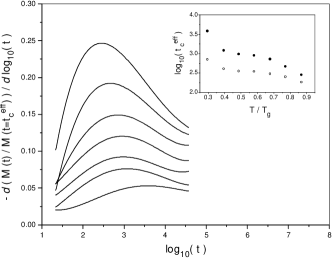
Figure 2: The logarithmic relaxation rate for the ZTRM. The measurement temperatures, from top to bottom, are $T/T_{g}=0.87,0.77,0.68,0.58,0.5,0.4$, and $0.3$. The inset shows temperature dependence of logarithms of the effective cooling time, $t_{c}^{e\!f\!f}$ (solid symbols), and the effective scaling time, $t_{s}^{e\!f\!f}$ (open symbols).

Even though the effective cooling time, $t_{c}^{e\!f\!f}$, corresponds to the maximum of the relaxation rate, it cannot be treated as a regular waiting time $t_{w}$. We have tried to scale each ZTRM curve with the relaxation curves for longer waiting times, using the $\mu$-scaling approach and taking $t_{c}^{e\!f\!f}$ as the scaling parameter. No value of $\mu$ can give even approximate scaling, especially at short times. It turns out, however, that the ZTRM curve can be merged with the other TRM curves (using the same $\mu$ as used for the longer waiting times), if a much shorter characteristic time for the ZTRM is introduced. We call this time the “effective scaling time”, $t_{s}^{e\!f\!f}$. It is several times shorter than the effective cooling time. The inset of Fig. 2 exhibits logarithms of $t_{c}^{e\!f\!f}$ and $t_{s}^{e\!f\!f}$ for different temperatures. The error bars for the logarithms are typically 0.1, but about 0.2 for the lowest temperature.

The fact that one can consider at least two characteristic times for the ZTRM agrees with what is expected from relaxation in the positive-temperature-cycle experiment. The spin-glass behavior at short observation times is governed by $t_{s}^{e\!f\!f}$, which can be associated with ordinary aging effects during the slow approach of the measurement temperature. However, the long-time relaxation is strongly influenced by the metastable states, separated by high barriers, resulting from the temperature change. Thus, the relaxation rate peaks at $t_{c}^{e\!f\!f}$, and not at $t_{s}^{e\!f\!f}$. This argument can be generalized to include the TRM experiments with finite waiting times. The logarithmic relaxation rate has a peak at $t_{w}^{e\!f\!f}$, the effective waiting time. It is well known that $t_{w}^{e\!f\!f}$ for the TRM is greater than $t_{w}$.nor00 We believe that this shift in the maximum of the relaxation rate is caused by those long-time metastable states, which are created during the cooling process.

It is important to note that memory of the initial state depends not only on the cooling protocol, but also on the overall complexity of the free-energy landscape. This can be illustrated by measurements of the ZTRM in the presence of a high constant field. The minimum possible overlap, $q_{min}(H)$, between two states increases with increasing magnetic field, $H$.par83 Therefore, certain constraints on barrier heights are imposed by the field, leading to a faster relaxation. The experiment is performed in the following way. First, the sample is cooled down to the measurement temperature at the field $H+\Delta H$. The field is changed to $H$, and the zero waiting time magnetization (ZTRM) is measured for some time. Second, the sample is warmed up to above $T_{g}$, and cooled down again, all in the presence of the same field $H$. The field-cooled magnetization (MFC) is measured for the same time. The difference of these two magnetizations is then fitted to a power law at long observation times: $ZTRM(t,H,\Delta H)-MFC(t,H)\propto t^{-\lambda(H)}$. The values of $H$ were varied from $50~{}Oe$ to $1000~{}Oe$. The field change was small, $\Delta H=10~{}Oe$, so that the response was always linear.

Fig. 3 exhibits the measured ZTRM and MFC decays for $H=500~{}Oe$. One can see that time dependence of the MFC cannot be neglected at high fields. The inset shows the relaxation exponent $\lambda(H)$. The exponent appears to be a linear function of $q_{min}\propto H^{2/3}$. This is not surprising, because its temperature dependence is also close to linear, and the AT critical line, $T_{g}-T_{c}(H)\propto H^{2/3}$, has a profound effect on spin-glass dynamics.zot01 The estimated value of $\lambda(H)$ near the AT line, which corresponds to $H_{AT}\sim 1400~{}Oe$ at this temperature, is $0.27\pm 0.03$. It is interesting that this number compares well with the Monte Carlo result, $\lambda\approx 0.25$, for the 3D EA model at zero magnetic field.kis96

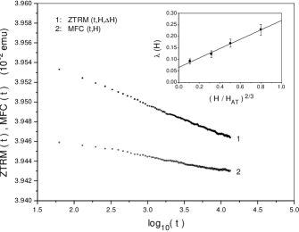
Figure 3: Time dependences of the ZTRM and MFC, measured at $T/T_{g}=0.79$ and $H=500~{}Oe$. The field change is $\Delta H=10~{}Oe$. The inset shows the relaxation exponent, $\lambda(H)$, as a function of $H^{2/3}$.

The observed increase in $\lambda(H)$ suggests that energy barriers, created by the cooling process, are lower, if cooling is performed in the presence of a high field. This happens because the accessible phase space is limited by $q_{min}(H)$. The low-field initial state in our experiments appears to be more complex, i.e. characterized by higher barriers, than the initial state in Monte Carlo simulations.

III.2 Subaging or superaging?

It was shown in Sec. II.A that the TRM relaxation can be decomposed into a sum of two decays: the IRM, which is a response of the system associated with the waiting time, $t_{w}$, and the ZTRM, which is a response of the initial state.

Fig. 4 displays the experimental TRM and ZTRM curves, and their difference, for $T/T_{g}=0.87$ and $t_{w}=1000~{}s$. One can see that the response of the initial state dominates the measured TRM relaxation. This effect is particularly pronounced at low temperatures, where thermally activated processes are slow. Fig. 4 suggests that the ZTRM cannot be neglected, nor can it be regarded as a constant. Therefore, the TRM and IRM relaxation curves will have different scaling properties, and should be studied simultaneously.

Figure 4: Experimental time dependence of the $\chi_{TRM}(t,t_{w})$ and $\chi_{IRM}(t,t_{w})$ for $T/T_{g}=0.87$ and $t_{w}=1000~{}s$. The TRM relaxation for zero waiting time is referred to as ZTRM. Note its large magnitude in comparison with the TRM for $t_{w}\neq 0$.

In this paper, we consider a multiplicative representation for the measured relaxation curves, in analogy with Eqs. (7) and (8):

$$\chi_{TRM}=\phi(t/t_{w})\,\rho_{TRM}(t,t_{w},t_{c})~{}~{};$$ (11)

$$\chi_{IRM}=\phi(t/t_{w})\,\rho_{IRM}(t,t_{w},t_{c})~{}~{}.$$ (12)

Here we made an assumption that both the TRM and the IRM are characterized by the same scaling part, $\phi(t/t_{w})$. This is certainly correct in the limit of very long waiting times, when the two functions are essentially equal. Analysis of experimental data, based on Eqs. (11) and (12), suggests that this approach works well on the real time scales.

Systematic departures from full $t/t_{w}$ scaling are described by the factors $\rho_{TRM}$ and $\rho_{IRM}$. If violations of $t/t_{w}$ scaling were only due to the quasiequilibrium behavior, these factors would depend only on the observation time, $t$. We assume, however, that there is an interplay between the cooling and waiting-time effects. Thus, we include the waiting time, $t_{w}$, and an additional argument $t_{c}$, which indicates dependence on the cooling process.

The correlation function, $C(t+t_{w},t_{w})$, defined by Eq. (1), is independent of $t_{w}$ at $t=0$. Numerical studies of the SK model demonstrate mar98 ; tak97 that the correlation curves for different waiting times, plotted versus $t/t_{w}$, cross at one point, corresponding to $t\approx t_{w}$. This is not surprising, because transition from the quasiequilibrium to the aging regime occurs at $t\approx t_{w}$, and the correlation at this point is near $q_{EA}$. If the linear response susceptibility depends on its time arguments only through the correlation function, i.e. $\chi=\chi(C)$, the susceptibility curves should also cross at one point. Experimental results do not exhibit this property. The TRM curves for long waiting times lie below the curves for short waiting times, when plotted vs. $t/t_{w}$. The IRM curves demonstrate the opposite behavior.

In the present paper, we normalize both the TRM and the IRM decays by one at $t=t_{w}$, and treat them as “normal” relaxation functions. This approach has several advantages. First, all departures from full $t/t_{w}$ scaling, reflected in the shapes of relaxation curves, can be observed clearly. Second, the shapes of TRM and IRM decays can be compared in detail, regardless of the fact that their magnitudes are different. Third, experimental results can be directly compared with results of numerical simulations. We believe that this approach is physically justified because the influence of the cooling process leads to systematic changes in the shapes of relaxation curves, as discussed in Sec. III.A. This method is different from the one, traditionally used to study $t/t_{w}$ scaling.vin96 ; oci85 It provides new insights into aging behavior of real spin glasses.

Fig. 5 exhibits the TRM and IRM relaxation curves, measured at $T/T_{g}=0.87$, for two waiting times, $t_{w}=1000~{}s$ and $t_{w}=6310~{}s$. The TRM data demonstrate the familiar subaging pattern: the relaxation, plotted versus $t/t_{w}$, is faster for the longer waiting time. The IRM results show a quite different behavior: the relaxation as a function of $t/t_{w}$ slows down as $t_{w}$ increases. This effect is called “superaging”. bou97

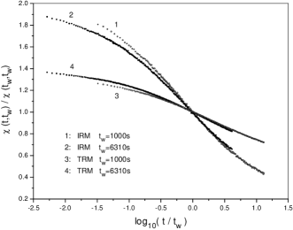
Figure 5: Relaxation curves $\chi_{IRM}(t,t_{w})$ and $\chi_{TRM}(t,t_{w})$ for two waiting times, normalized by one at $t=t_{w}$. The temperature is $T/T_{g}=0.87$. The IRM decay as a function of $t/t_{w}$ is slower for longer waiting times (“superaging”). The TRM decay is faster for longer waiting times (“subaging”).

The phenomenon of superaging may seem rather unusual from an experimentalist’s point of view, because it has never been observed in TRM experiments. It turns out, however, that this is a predominant effect in Monte Carlo simulations. Fig. 4 in Marinari et al.,mar98 Fig. 4 in Takayama et al.,tak97 and Fig. 4 in Cugliandolo et al.rit94 clearly demonstrate the superaging behavior. In all these simulations of the SK model, the correlation function, $C(t+t_{w},t_{w})$, plotted versus $t/t_{w}$, decays slower for longer waiting times. In the case of the EA model, it is more difficult to distinguish between the subaging and superaging effects, because the correlation curves exhibit good $t/t_{w}$ scaling in the aging regime. However, the relaxation exponent $\lambda(T,t_{w})$, defined as $C(t+t_{w},t_{w})\propto t^{-\lambda}$ for $t\gg t_{w}$, decreases slightly with increasing $t_{w}$, according to Fig. 2 in Kisker et al.kis96 This fact suggests that the superaging behavior appears in the EA model as well.

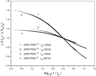
Figure 6: Factorization of the relaxation curves from Fig. 5. $f=(\chi_{IRM}\,\chi_{TRM})^{1/2}$ is an average over two different initial conditions, which shows systematic improvement in $t/t_{w}$ scaling. $g=(\chi_{IRM}/\chi_{TRM})^{1/2}$ describes departures from the average and does not scale well.

Because the experimental TRM and IRM curves have the opposite scaling properties (subaging versus superaging), the functions $\rho_{TRM}$ and $\rho_{IRM}$, describing departures from full $t/t_{w}$ scaling in Eqs. (11) and (12), may be expected to have inverse effects on the function $\phi(t/t_{w})$. Following this observation, we define two auxiliary functions, $f$ and $g$. The function $f$ is a geometric mean of $\chi_{TRM}$ and $\chi_{IRM}$, and the function $g$ describes departures from this mean:

$$f(t,t_{w},t_{c})=(\chi_{IRM}\,\chi_{TRM})^{1/2}~{}~{};$$ (13)

$$g(t,t_{w},t_{c})=(\chi_{IRM}/\chi_{TRM})^{1/2}~{}~{}.$$ (14)

With this definition of $f$, the scaling part, $\phi(t/t_{w})$, is left unchanged, while deviations from full scaling are averaged out, at least partially. Physically, the function $f$ represents an average over two different initial conditions. Of course, if both $\chi_{TRM}$ and $\chi_{IRM}$ are normalized by one at $t=t_{w}$, their geometric mean is close to the arithmetic mean. The IRM and TRM relaxation curves can be factorized as follows:

$$\chi_{IRM}=f\,g~{}~{};~{}~{}~{}~{}~{}~{}~{}\chi_{TRM}=f/g~{}~{}.$$ (15)

Fig. 6 exhibits the functions $f$ and $g$ for $T/T_{g}=0.87$. Both of them demonstrate the superaging behavior, but the function $f$ shows much better $t/t_{w}$ scaling. The function $g$ is responsible for the faster relaxation in the IRM experiments, and the slower relaxation in the TRM experiments.

III.3 Comparison of TRM and IRM

In order to make the above arguments quantitative, we analyze the $t/t_{w}$ scaling of relaxation curves using the $\mu$-scaling approach, discussed in Sec. II.B. We optimize $\mu$ to achieve the best possible scaling over a wide range of observation times, with particular attention to the aging regime, $t>t_{w}$. Inclusion of the quasiequilibrium decay with the exponent $\alpha$ improves scaling at short times, but it does not help at longer times. In the present analysis, the quasiequilibrium behavior is not taken into account explicitly. This gives values of $\mu$ a little further from unity, but does not affect any conclusions about scaling in the aging regime.

Fig. 7 exhibits values of the parameter $\mu$ for the TRM, IRM, and their combinations.

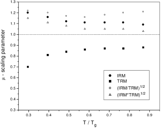
Figure 7: The scaling parameter $\mu$ as a function of temperature for different relaxation functions. Note that $\mu<1$ for the TRM (“subaging”), and $\mu>1$ for the IRM (“superaging”).

In the case of the TRM, $\mu$ lies between 0.8 and 0.9 for relatively high temperatures, but drops visibly at low temperatures, $T/T_{g}<0.4$. Similar results have been obtained for various spin-glass samples.vin96 ; oci85 ; alb87 The error bars in our analysis are typically 0.02. At the lowest temperature, however, they are about 0.1 for the TRM, and about 0.05 for the IRM.

The values of $\mu$ for the IRM are greater than unity. They are near 1.1, but tend to increase at low temperatures. According to Fig. 7, there is a certain symmetry with respect to $\mu=1$ between the values of $\mu$ for the TRM and the IRM. We have also found that, in the case of the IRM, the parameter $\mu$ is very sensitive to any imperfections of the scaling analysis. For example, if the actual observation time is slightly longer, than the time $t$, used in the analysis, the corresponding value of $\mu$ will seem closer to unity. This issue is important when a superconducting magnet is used, because it takes some time to warm up the persistent switch, and then to cool it down again. The results for the TRM are less sensitive to these effects.

Fig. 7 also displays $\mu$ for the functions $f$ and $g$, given by Eqs. (13) and (14). The value of $\mu$ for the function $f$ is about 1.05, while for the function $g$ it is near 1.20. Thus, both the TRM and the IRM relaxations can be presented as products of two factors, according to Eq. (15). The rapidly changing $f$ exhibits fairly good $t/t_{w}$ scaling. The relatively slow $g$ describes departures from this scaling. This function becomes closer to a constant as $t_{w}$ increases, suggesting that both the TRM and the IRM curves scale better for longer waiting times. At low temperatures, however, the differences between $f$ and $g$ tend to diminish.

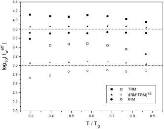
Figure 8: Logarithm of the effective waiting time, $t_{w}^{e\!f\!f}$, as a function of temperature. The solid symbols correspond to $t_{w}=6310~{}s$, and the open symbols – to $t_{w}=1000~{}s$. Note that $t_{w}^{e\!f\!f}>t_{w}$ for the TRM, and $t_{w}^{e\!f\!f}<t_{w}$ for the IRM.

Fig. 8 exhibits values of logarithm of the effective waiting time, $t_{w}^{e\!f\!f}$, for different relaxation functions. The relaxation curves were fitted using a 5-order polynomial fit, and then differentiated with respect to $\log_{10}(t)$. The effective waiting time, $t_{w}^{e\!f\!f}$, corresponds to the maximum of this derivative. The error bars for $\log_{10}(t_{w}^{e\!f\!f})$ are typically 0.05, but about 0.1 for the lowest temperature. It can be seen from Fig. 8, that $t_{w}^{e\!f\!f}>t_{w}$ for the TRM, but $t_{w}^{e\!f\!f}<t_{w}$ for the IRM. The values of the effective waiting time for the function $f$ are greater than $t_{w}$, but they all differ from $t_{w}$ by less than 3%. Therefore, the average of the TRM and the IRM gives better results for the effective waiting time as well.

Fig. 9 provides a further insight into the nature of these phenomena. It displays values of the relaxation exponent, $\lambda(T,t_{w})$, defined through $\chi(t,t_{w})\propto t^{-\lambda(T,t_{w})}$ for $t\gg t_{w}$. This definition is based on the fact that time dependence of spin-glass relaxation is essentially algebraic in the aging regime.bou92 ; bou95 ; kis96 The value of $\lambda(T,t_{w})$ is determined from the slope of the linear fit to $\log_{10}(\chi)$ as a function of $\log_{10}(t)$. Because of time limitations in our experiments, the fitting was performed in the interval $t/t_{w}=1.5...10$ for $t_{w}=1000~{}s$, and in the interval $t/t_{w}=1.5...5$ for $t_{w}=6310~{}s$. In the case of the ZTRM, the effective cooling time, $t_{c}^{e\!f\!f}$, was used instead of $t_{w}$. The algebraic approximation works well, and the error bars for the relaxation exponents are about 1%.

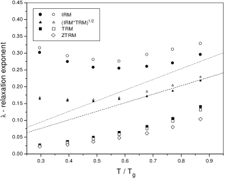
Figure 9: The relaxation exponent, $\lambda(T,t_{w})$, as a function of temperature. The solid symbols correspond to $t_{w}=6310~{}s$, and the open symbols – to $t_{w}=1000~{}s$. The open diamonds denote $\lambda$ for the experimental ZTRM. The upper and lower straight lines are Monte Carlo results for $t_{w}=0$ and $t_{w}=1000~{}mcs$, respectively (from Kisker et al., Ref. 13).

The first conclusion one can draw from Fig. 9 is that the zero waiting time decay, ZTRM, is the slowest relaxation measured in the aging regime. This result is in sharp contradiction with results of numerical simulations, which show that the zero waiting time decay is the fastest possible relaxation. The dotted (upper) line in Fig. 9 represents $\lambda(T)$ for $t_{w}=0$ from the Monte Carlo studies of the EA model by Kisker et al.kis96 Our experimental values of the $\lambda(T)$ for the ZTRM are about 3 times lower. We have also tried to estimate the relaxation exponent for the SK model, using numerical results of Marinari et al.mar98 and Takayama et al.tak97 , and fitting them in the interval $t/t_{w}=1...100$. In the first case, for $T/T_{g}=0.5$ and $t_{w}=8~{}mcs$, we find $\lambda(T,t_{w})\approx 0.15$. In the second case, for $T/T_{g}=0.4$ and $t_{w}=16~{}mcs$, we determine $\lambda(T,t_{w})\approx 0.20$. These numbers are similar to those for the EA model.

Fig. 9 demonstrates that the TRM decay at $t>t_{w}$ becomes faster as the waiting time increases, while the IRM relaxation becomes slower. The corresponding values of $\lambda(T,t_{w})$ move towards each other and towards the dashed (lower) line, which represents numerical results for the EA model with $t_{w}=1000~{}mcs$. kis96 One can see that the function $f$, the average of the TRM and the IRM, has relaxation exponents, which (at relatively high temperatures) are very close to those from the Monte Carlo simulations. These exponents decrease slightly with increasing $t_{w}$, as the numerical results do.

III.4 A possible origin of $\mu$

We are now in a position to offer a tentative explanation for these phenomena. It is based on two observations. First, there is a certain degree of symmetry between the TRM and the IRM with respect to the “ideal” case, according to Figs. 7-9. Of course, this symmetry is not exact and depends on a particular realization of the cooling process. Second, when the waiting time, $t_{w}$, is very large, the TRM and IRM become essentially equal, according to Eq. (6). This situation corresponds to the weak long-term memory.cug94 ; bou97 These two observations suggest that the experimental TRM and IRM decays approximate the true spin-glass relaxation from the opposite sides.

Let us first consider a typical TRM experiment. When the cooling is over, a number of metastable states, separated by free-energy barriers of different heights, are already populated. We shall refer to them loosely as the initial state. The response of this state, the ZTRM, is slow and cannot be characterized by a single well-defined time scale. The initial state is not random: it has already evolved towards some equilibrium state, and this makes it energetically favorable. During the waiting time, evolution continues in the same direction. Thus, in the case of the TRM, aging and cooling effects work together. The spin-glass state appears to be older. The characteristic barrier is higher than $\Delta(T,t_{w})=k_{B}T\ln(t_{w}/\tau_{0})$, the barrier, associated with the waiting time $t_{w}$.led91 The TRM decay is slower than the ideal $t_{w}$-dependent relaxation, which can be characterized by some exponent $\lambda_{0}$. As the waiting time increases, influence of the initial state diminishes. The relaxation, plotted versus $t/t_{w}$, becomes faster, and its dependence on $t_{w}$ – stronger. This leads to the subaging behavior. Therefore, for the TRM experiments, we would expect $\mu<1$, $t_{w}^{eff}>t_{w}$, and $\lambda<\lambda_{0}$.

Let us now discuss a typical IRM experiment. In this case, a small magnetic field is applied after the cooling process and before the waiting time. The initial state, created by the cooling, is again partially equilibrated. The subsequent field change makes it energetically unfavorable. This is a consequence of chaotic nature of the spin-glass state with respect to magnetic field. Even if the field change is very small, the new equilibrium state (reached at the end of the relaxation process) is very different from the old one.par83 The system can no longer evolve in the same direction. Moreover, it has to escape from the initial state. Therefore, in the case of the IRM, aging and cooling effects work against each other. During the same waiting time, $t_{w}$, the system will have to overcome barriers, produced by the cooling process, and explore a different part of the phase space, thus exhibiting aging. As a result, the spin-glass state looks younger. The characteristic barrier, corresponding to the waiting time, $t_{w}$, is now lower than $\Delta(T,t_{w})$ for the ideal aging. The IRM decay is faster than the ideal relaxation. However, memory of the initial state weakens as the waiting time increases. The IRM relaxation as a function of $t/t_{w}$ becomes slower and more dependent on $t_{w}$. This leads to the superaging behavior. Therefore, the IRM experiments should yield $\mu>1$, $t_{w}^{eff}<t_{w}$, and $\lambda>\lambda_{0}$.

If this explanation is reasonable, the observed difference in scaling properties of the TRM and the IRM is a result of the different initial conditions for aging. Departures from full $t/t_{w}$ scaling are present in the aging regime not because something goes wrong at long waiting times (e.g. the interrupted agingbou94 ), but because results for short waiting times are strongly affected by the initial state. An average over different initial conditions should improve $t/t_{w}$ scaling.

Presence of many metastable states, separated by high barriers, is a well-known problem in Monte Carlo simulations, involving thermolization of large samples. The system easily gets trapped in a metastable state and cannot efficiently explore the entire phase space to find the ground state.mar01 The cooling process in spin-glass experiments gives a similar result: the system is trapped before the waiting time begins. However, Monte Carlo studies of aging phenomena do not simulate the cooling protocol. The simulations are started directly at the measurement temperature from a random initial configuration, and results are averaged over different initial conditions. kis96 ; rit01 ; mar98 ; tak97 ; rit94 This may be the reason why the subaging behavior is not normally observed in numerical simulations. Moreover, the random initial configuration corresponds to zero net magnetization. This means that Monte Carlo studies are probably closer to the IRM, than to the TRM, experiments.rit94 The difference between the two is not very important, if memory of the initial state disappears quickly. This, however, is not the case in real experiments.

The factorization of the TRM and IRM relaxation curves, Eq. (15), allows us to illustrate a possible origin of $\mu$ in a simple way. The functions $f$ and $g$, Eqs. (13) and (14), can be approximated algebraically in the aging regime:

$$f\propto(t/\,t_{w}^{\,\mu_{1}})^{-\lambda_{1}}~{}~{};~{}~{}~{}~{}~{}~{}~{}~{}~{}g\propto(t/\,t_{w}^{\,\mu_{2}})^{-\lambda_{2}}~{}~{}.$$ (16)

It follows from Eq. (15) that the relaxation exponent for the IRM is $\lambda_{1}+\lambda_{2}$, while the exponent for the TRM is $\lambda_{1}-\lambda_{2}$. The corresponding values of $\mu$ depend on the ratio $r=\lambda_{2}/\lambda_{1}$:

$$\mu_{IRM}=(\mu_{1}+\mu_{2}\,r)/\,(1+r)~{}~{};$$ (17)

$$\mu_{TRM}=(\mu_{1}-\mu_{2}\,r)/\,(1-r)~{}~{}.$$ (18)

The experimental values of $\mu_{1}$ and $\mu_{2}$ are exhibited in Fig. 7. The exponents $\lambda_{1}$ are displayed in Fig. 9, and the ratios $r=\lambda_{2}/\lambda_{1}$ – in the inset of Fig. 10.

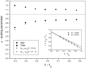
Figure 10: Illustration of a possible origin of $\mu$. Parameters $\mu_{1}$ and $\lambda_{1}$ correspond to $f=(\chi_{IRM}\,\chi_{TRM})^{1/2}$, while $\mu_{2}$ and $\lambda_{2}$ correspond to $g=(\chi_{IRM}/\chi_{TRM})^{1/2}$.

The values of $\mu$ for the IRM and the TRM, determined from Eqs. (17) and (18), are shown in the main body of Fig. 10. They compare well with the experimental values of $\mu$, obtained from analysis of the actual relaxation curves. This comparison demonstrates how the function $g$, which exhibits strong superaging properties with $\mu_{2}\sim 1.2$, leads to $\mu\sim 0.9$ for the TRM, and $\mu\sim 1.1$ for the IRM. The results in Fig. 10 were obtained using values of $r$ for $t_{w}=1000~{}s$. The values of $r$ for $t_{w}=6310~{}s$ give similar numbers. For the sake of simplicity, the observation time, $t$, is used in Eq. (16) instead of the $\mu$-dependent effective time, $t_{e}$, given by Eq. (9). The fact that Eqs. (17) and (18) yield values of $\mu$ close to the their actual values suggests that this approach is justified.

Appearance of the $\mu$-scaling can be explained in the following way. Imagine that there is a function that exhibits good $t/t_{w}$ scaling. Let us also assume that effect of initial conditions is described by another function, which does not scale well. This second function will necessarily display superaging behavior, approaching a constant as $t_{w}$ increases. Imagine also that both these functions can be approximated by power laws of time, which is often the case in spin-glass dynamics. If the first function is fast, and the second function is slow, the resulting decay will exhibit the $\mu$-scaling with $\mu$ not far from unity. Of course, this is only one of possible scenarios.

According to Eqs. (17) and (18), in order to achieve the best scaling of both the TRM and the IRM (with $\mu$ close to unity), one has to make the ratio $r=\lambda_{2}/\lambda_{1}$ as small as possible. The inset of Fig. 10 suggests that $r$ decreases with temperature and can be well approximated by a linear function of $T/T_{g}$. It also diminishes with increasing $t_{w}$. Thus, higher temperatures and longer waiting times should improve $t/t_{w}$ scaling of measured relaxation curves.

Eq. (18) also predicts that the quality of $\mu$-scaling of the TRM curves should become worse as $r\rightarrow 1$ and $\mu_{1}\rightarrow\mu_{2}$, because of the uncertainty 0/0. This happens at low temperatures: the experimental values of $\mu$ for the TRM drop sharply and their error bars increase considerably. The physical reason for this is simple. The TRM relaxation at low temperatures is completely dominated by the ZTRM, which is very slow. The waiting time effects become almost indistinguishable, and the $t/t_{w}$ scaling does not make much sense anymore. In this case, the TRM is nearly constant, and both $f$ and $g$, Eqs. (13) and (14), are governed by the IRM. Therefore, the simple average of the TRM and IRM does not give much better scaling at low temperatures, as seen in Fig. 7.

These results can be interpreted in terms of an effective change in barrier heights. Let us consider the logarithmic relaxation rates: $S_{TRM}=-\partial\chi_{TRM}/\partial\ln(t)$ and $S_{IRM}=-\partial\chi_{IRM}/\partial\ln(t)$. As usually, we assume that both $\chi_{TRM}$ and $\chi_{IRM}$ are normalized by one at $t=t_{w}$ before differentiation is performed. A ratio of $S_{TRM}$ and $S_{IRM}$ can be regarded as a probability of overcoming a barrier:

$$d\chi_{TRM}/\,d\chi_{IRM}=\exp(-\Delta_{0}/k_{B}T)~{}~{}.$$ (19)

This formula defines the effective barrier $\Delta_{0}(t,t_{w})$, describing the difference in relaxation rates for two different initial conditions.

Fig. 11 exhibits values of $\Delta_{0}/k_{B}T$ at $t=t_{w}$, extracted from the experimental data according to Eq. (19). One can see that they grow steadily as temperature decreases. They are also comparable with differences between the values of $\ln(t_{w}^{e\!f\!f})$ for the TRM and the IRM. Values of $\Delta_{0}(t_{w},t_{w})$ are displayed in the inset of Fig. 11. They change only slightly over a wide range of temperatures, and decrease with increasing $t_{w}$. The error bars for $\Delta_{0}$ are about 0.05.

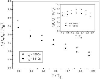
Figure 11: The effective barrier $\Delta_{0}$, describing difference in relaxation rates for the TRM and the IRM, at $t=t_{w}$. Note that it is almost independent of temperature, as shown in the inset.

It has been shown experimentally that a change in a barrier height, $\delta\Delta$, under a temperature change, $\delta T$, is independent of temperature.ham92 The same appears to be true for $\Delta_{0}$, which corresponds to an average change in barrier heights due to the change in initial conditions. This fact suggests that $\Delta_{0}$ is a result of cooling. Both the TRM and the IRM are influenced by the cooling process, and it is mainly this influence, that leads to systematic deviations from full $t/t_{w}$ scaling in the aging regime. As the waiting time increases, $\Delta_{0}$ diminishes, which means that memory of the initial state is gradually washed away by the aging process.

It has been already mentioned that evolution of the system during the waiting time $t_{w}$ can be characterized by the effective barrier $\Delta(T,t_{w})=k_{B}T\ln(t_{w}/\tau_{0})$. The barriers are raised by $\Delta_{TRM}$ for the TRM, and reduced by $\Delta_{IRM}$ for the IRM. The average difference in barrier heights for these experimental protocols is $\Delta_{0}=\Delta_{TRM}+\Delta_{IRM}$. Using Eq. (19), one can determine $\Delta_{0}$ only. Fig. 8 suggests that $\Delta_{TRM}$ and $\Delta_{IRM}$ may be different, but have similar properties. Therefore, what is true for $\Delta_{0}$, is likely to be true for $\Delta_{TRM}$ and $\Delta_{IRM}$ taken separately.

The characteristic barrier, $\Delta(T,t_{w})$, decreases with decreasing temperature, because it corresponds to thermally activated aging dynamics. The barrier $\Delta_{0}$ is almost independent of temperature, presumably because it is related to the cooling process. Therefore, departures from full $t/t_{w}$ scaling should become more pronounced as temperature is lowered. Even if the cooling is fast, yielding small $\Delta_{0}$, it will always be possible to find a sufficiently low measurement temperature, $T$, so that $\Delta(T,t_{w})\sim\Delta_{0}$, and the $t/t_{w}$ scaling is strongly violated. According to this argument, the sharp drop in $\mu$ for the TRM at low temperatures is a natural consequence of cooling effects.

Some of the measurements, discussed above, have been repeated at CEA Saclay. A SQUID susceptometer S600 by Cryogenics Ltd (UK) was used for this purpose. The cooling process, which is a unique characteristic of an apparatus, was somewhat different from the one exhibited in Fig. 1. The experimental data, however, are consistent with the results, reported in this paper.

IV Conclusion

There are many different approaches to analysis of $t/t_{w}$ scaling in spin glasses. In this paper, one more method is proposed. It is based on the idea that the departures from $t/t_{w}$ scaling, observed experimentally in the aging regime, may reflect the influence of the cooling process. This means that the thermal history of the spin-glass state cannot be neglected in analysis of aging phenomena. The initial condition for aging is not random in spin-glass experiments, and has a profound effect on scaling properties of measured relaxation. It would be incorrect to say that the cooling effects are spurious. They are as important, as the aging phenomena. This is because they reflect the hierarchical nature of spin-glass dynamics,bou02 revealed by temperature-variation experiments.

The approach, used in this paper, is based on the detailed comparison of time scaling properties of the TRM and the IRM. We argue that, because of strong memory of the initial state, neither of these functions represents the true $t_{w}$-dependent relaxation. Even though they are characterized by the same waiting time, their $t/t_{w}$ scaling properties are remarkably different. We exploit this difference by taking an average of $\chi_{TRM}$ and $\chi_{IRM}$. This averaging over different initial conditions leads to systematic improvement in $t/t_{w}$ scaling. Factorization of measured relaxation functions allows us to explain scaling properties of both the TRM and the IRM in a unique way. Our results suggest that the observed deviations from $t/t_{w}$ scaling in the aging regime are largely due to cooling effects. The interrupted aging,bou94 which is another possible reason for the lack of scaling, may be expected to play a role at longer waiting times, especially in polycrystalline samples.

The conclusions, reached in this paper, are by no means final. Their verification requires experiments in which different cooling protocols in the immediate vicinity of the measurement temperature can be implemented. Another option is a rapid field quench from above the AT line. Monte Carlo studies, including simulations of the cooling process in addition to aging effects, may also be very helpful. The problem of $t/t_{w}$ scaling in spin-glass dynamics deserves further experimental and theoretical investigation.

NOTE. After this paper had been completed, we received a preprint by Berthier and Bouchaud,ber02 devoted to numerical studies of the Edwards-Anderson model in 3 and 4 dimensions. One of their conclusions is that “a finite cooling rate effect…leads to an apparent sub-aging behavior for the correlation function, instead of the super-aging that holds for an infinitely fast quench”. This is in agreement with the conclusion of the present paper that $t/t_{w}$ scaling properties strongly depend on the initial condition.

- (1) L. Lundgren, P. Svedlindh, P. Nordblad, and O. Beckman, Phys. Rev. Lett. 51, 911 (1983).
- (2) E. Vincent, J. Hammann, M. Ocio, J.-P. Bouchaud, and L. F. Cugliandolo, in Complex Behavior of Glassy Systems, ed. by M. Rubi, Springer Verlag Lecture Notes in Physics, vol. 492 (Springer Verlag, Berlin, 1997). Available as cond-mat/9607224.
- (3) M. Ocio, M. Alba, and J. Hammann, J. Phys. Lett. (France) 46, L1101 (1985); M. Alba, M. Ocio, and J. Hammann, Europhys. Lett. 2, 45 (1986).
- (4) M. Alba, J. Hammann, M. Ocio, and Ph. Refregier, J. Appl. Phys. 61, 3683 (1987).
- (5) J.-P. Bouchaud, E. Vincent, and J. Hammann, J. Phys. I (France) 4, 139 (1994).
- (6) B. Rinn, P. Maass, and J.-P. Bouchaud, Phys. Rev. Lett. 84, 5403 (2000); L. Berthier, Eur. Phys. J. B 17, 689 (2000).
- (7) J.-P. Bouchaud, J. Phys. I (France) 2, 1705 (1992).
- (8) J.-P. Bouchaud and D. S. Dean, J. Phys. I (France) 5, 265 (1995).
- (9) J.-P. Bouchaud, L. F. Cugliandolo, J. Kurchan, and M. Mezard, in Spin Glasses and Random Fields, edited by A. P. Young (World Scientific, Singapore, 1997).
- (10) L. F. Cugliandolo and J. Kurchan, Phys. Rev. Lett. 71, 173 (1993).
- (11) L. F. Cugliandolo and J. Kurchan, J. Phys. A 27, 5749 (1994).
- (12) L. F. Cugliandolo and J. Kurchan, Phys. Rev. B 60, 922 (1999).
- (13) J. Kisker, L. Santen, M. Schreckenberg, and H. Rieger, Phys. Rev. B 53, 6418 (1996); H. Rieger, Physica A 224, 267 (1996); H. Rieger, J. Phys. A 26, L615 (1993).
- (14) M. Picco, F. Ricci-Tersenghi, and F. Ritort, Eur. Phys. J. B 21, 211 (2001).
- (15) E. Marinari, G. Parisi, and D. Rossetti, Eur. Phys. J. B 2, 495 (1998).
- (16) H. Takayama, H. Yoshino, and K. Hukushima, J. Phys. A 30, 3891 (1997).
- (17) L. F. Cugliandolo, J. Kurchan, and F. Ritort, Phys. Rev. B 49, 6331 (1994).
- (18) M. Picco, F. Ricci-Tersenghi, and F. Ritort, Phys. Rev. B 63, 174412 (2001).
- (19) K. Jonason, P. Nordblad, E. Vincent, J. Hammann, and J.-P. Bouchaud, Eur. Phys. J. B 13, 99 (2000).
- (20) We do not consider a quench from a high magnetic field here. For details, see P. Nordblad, P. Svedlindh, P. Granberg, and L. Lundgren, Phys. Rev. B 35, 7150 (1987); F. Lefloch, J. Hammann, M. Ocio, and E. Vincent, Physica B 203, 63 (1994).
- (21) Ph. Refregier, E. Vincent, J. Hammann, and M. Ocio, J. Phys. (France) 48, 1533 (1987).
- (22) M. Lederman, R. Orbach, J. M. Hammann, M. Ocio, and E. Vincent, Phys. Rev. B 44, 7403 (1991).
- (23) J. Hammann, M. Ocio, E. Vincent, M. Lederman, and R. Orbach, J. Mag. Magn. Mat. 104, 1617 (1992).
- (24) K. Jonason and P. Nordblad, Physica B 279, 334 (2000).
- (25) L. Lundgren, P. Nordblad, and L. Sandlund, Europhys. Lett. 1, 529 (1986).
- (26) S. Franz and H. Rieger, J. Stat. Phys. 79, 749 (1995).
- (27) Note that a comprehensive description of results from magnetic noise, relaxation, and susceptibility measurements suggests that a quasiequilibrium factor , where is a constant, should be used instead of , as explained in Ref. 4 above.
- (28) V. S. Zotev and R. Orbach, cond-mat/0112489.
- (29) J.-P. Bouchaud, V. Dupuis, J. Hammann, and E. Vincent, Phys. Rev. B 65, 024439 (2002).
- (30) G. Parisi, Phys. Rev. Lett. 50, 1946 (1983); F. Ritort, Phys. Rev. B 50, 6844 (1994).
- (31) E. Marinari, G. Parisi, F. Ricci-Tersenghi, and F. Zuliani, J. Phys. A 34, 383 (2001).
- (32) L. Berthier and J.-P. Bouchaud, cond-mat/0202069.