Evidence against a glass transition in the 10-state short range Potts glass
Claudio Brangian¹, Walter Kob², and Kurt Binder¹

¹ Institut für Physik, Johannes-Gutenberg-Universität Mainz, Staudinger Weg 7,

D-55099 Mainz, Germany

² Laboratoire des Verres, Université Montpellier II, F-34095 Montpellier, France

We present the results of Monte Carlo simulations of two different 10-state Potts glasses with random nearest neighbor interactions on a simple cubic lattice. In the first model the interactions come from a $\pm J$ distribution and in the second model from a Gaussian one, and in both cases the first two moments of the distribution are chosen to be equal to $J_{0}=-1$ and $\Delta J=1$. At low temperatures the spin autocorrelation function for the $\pm J$ model relaxes in several steps whereas the one for the Gaussian model shows only one. In both systems the relaxation time increases like an Arrhenius law. Unlike the infinite range model, there are only very weak finite size effects and there is no evidence that a dynamical or a static transition exists at a finite temperature.

PACS numbers: 64.70.Pf, 75.10.Nr, 75.50.Lk

In recent years generalized spin-glass-type models such as the $p$-spin model with $p\geq 3$ or the Potts glass with $p>4$, have found a large attention 1 ; 2 ; 3 ; 4 ; 5 ; 6 ; 7 ; 8 ; 9 ; crisanti00 ; 10 ; 11 ; 12 as prototype models for the structural glass transition 13 ; 14 ; 15 ; 16 ; 17 ; 18 . In the case of infinite range interactions, i.e. mean field, these models can be solved exactly and it has been shown that they have a dynamical as well as a static transition at a temperature $T_{D}$ and $T_{0}$, respectively 1 ; 2 ; 3 ; 4 ; 5 ; 6 ; 7 ; 8 ; 9 ; crisanti00 ; 10 ; 11 ; 12 . At $T_{D}$ the relaxation times diverge but no singularity of any kind occurs in the static properties, whereas at $T_{0}$ a nonzero static glass order parameter appears discontinuously. Close to $T_{D}$ the time and temperature dependence of the spin autocorrelation function is described by the same type of mode coupling equations 3 ; 7 that have been proposed by the idealized version of mode coupling theory (MCT) 14 ; 15 for the structural glass transition which suggests a fundamental connection between these rather abstract spin models and real structural glasses.

Now it is well known that for real glasses the divergence of the relaxation times predicted by MCT is rounded off since thermally activated processes, which are not taken into account by this version of the theory, become important 14 ; 15 . This is in contrast to the mean field case because there these processes are completely suppressed since the barriers in the (free) energy landscape become infinitely high if $T<T_{D}$. To what extend the static transition that exists in mean field can be seen also in the real system, is a problem whose answer is still controversial 9 ; 16 ; 17 ; 18 .

In the present paper, we investigate whether the transitions present in the case of a mean field 10-state Potts glass are also found if the interactions are short ranged. The mean field model has recently been studied in great detail by means of Monte Carlo methods and the results are in good qualitative agreement with the main predictions of the one-step replica symmetry breaking theory 1 ; 2 ; 4 ; 6 , although very strong finite size effects occur, the nature of which are not fully understood 11 .

The Hamiltonian of the short range model is

$${\mathcal{H}}=-\sum_{\langle i,j\rangle}J_{ij}(p\;\delta_{\sigma_{i}\sigma_{j}}-1)\;.$$ (1)

The Potts spins $\sigma_{i}$ on the lattice sites $i$ of the simple cubic lattice take $p$ discrete values, $\sigma_{i}\in\{1,2,\ldots,p\}$, and the index $j$ runs over the six nearest neighbors of site $i$. The exchange constants $J_{ij}$ are taken either from a bimodal distribution

$$P(J_{ij})=x\delta(J_{ij}-J)+(1-x)\delta(J_{ij}+J)$$ (2)

or a Gaussian distribution

$$P(J_{ij})=[\sqrt{2\pi}(\Delta J)]^{-1}\exp\{-(J_{ij}-J_{0})^{2}/2(\Delta J)^{2}\}.$$ (3)

In both cases the first two moments are chosen to be $J_{0}=[J_{ij}]_{av}=-1$ and $(\Delta J)^{2}=[J_{ij}^{2}]_{av}-[J_{ij}]^{2}_{av}=+1$. (For $p=10$, a sufficiently negative $J_{0}$ is necessary to avoid ferromagnetic order and we have indeed found that neither the magnetization nor the magnetic susceptibility show any sign of ferromagnetic ordering 12 ).) For the distribution given by Eq. (2) this choice means $J=\sqrt{2}$ and $x=(1-1/\sqrt{2})/2\approx 0.146$. We carry out Monte Carlo runs with the standard heat-bath algorithm 19 making up to $10^{8}$ Monte Carlo steps (MCS) per spin (for equilibration as well as production), with lattices of linear dimensions $L=6$, $L=10$ and $L=16$, and using periodic boundary conditions. The average over the quenched disorder $[\cdots]_{av}$ is realized by averaging over $100$ independent realizations of the system for $L=6$ and $10$ and over 50 realizations for $L=16$. For $T=1.3$ and 1.4 and $L=10$ only 10 realizations were used. In the following we will set the Boltzmann constant $k_{B}\equiv 1$ and measure temperature in units of $\Delta J$.

In Fig. 1 we show the temperature dependence of the energy per spin $e(T)$ and of the specific heat $c(T)$, for the model given by Eq. (2). Both quantities seem to be essentially independent of system size, in stark contrast to the results for the mean field case 11 . Furthermore we see that for $T\leq 2$ the energy is basically constant and we have found that at low $T$ the temperature dependence of the specific heat is of the form $(\Delta/T)^{2}\exp(-\Delta/T)$, with $\Delta\approx 14$, i.e. a dependence expected for a two-level system with asymmetry $\Delta$. Thus we conclude that this data does not show any evidence that in the temperature range investigated a static transition occurs.

A similar conclusion is reached from the $T-$dependence of the spin glass susceptibility $\chi_{SG}=N[\langle q^{2}\rangle]_{av}/(p-1)$. Here the symmetrized order parameter $q$ is defined as 10 ; 11

$$q=\sqrt{\frac{1}{p-1}\,\sum\limits_{\mu,\nu=1}^{p-1}(q^{\mu\nu})^{2}}\quad\mbox{with}\quad q^{\mu\nu}\equiv L^{-3}\sum\limits_{i}(\vec{S}_{i,\alpha})^{\mu}({\vec{S}_{i,\beta}})^{\nu},\quad\mu,\nu=1,2,\ldots,p-1\quad,$$ (4)

and the spins $\vec{S}_{i,\alpha}$ refer to the simplex representation of the Potts spin $\sigma_{i}$ in replica $\alpha$ simplex_ref . (Note that in order to define an order parameter it is necessary to consider two replicas of the system, i.e. two systems with the same realization of the disorder.) Figure 2a shows the $T-$ dependence of $\chi_{SG}$ and we see that this quantity is almost independent of $L$. Furthermore we recognize that $\chi_{SG}$ remains finite even as $T\rightarrow 0$. Figure 2b shows the (scaled) first moment of $q$ and we conclude that it decreases like $1/\sqrt{L^{3}}$, i.e. shows a trivial size dependence for all $T$. Also an analysis of fourth order cumulants (not shown here) confirms the conclusion that no static transition occurs 12 . Similar results are found for the model with Gaussian distribution, Eq. (3).

In order to see whether this model has a dynamic transition at a finite temperature we consider the time autocorrelation function of the Potts spins:

$$C(t)=[L^{3}(p-1)]^{-1}\sum_{i=1}^{L^{3}}[\langle\vec{S}_{i}(t^{\prime})\cdot\vec{S}_{i}(t^{\prime}+t)\rangle]_{av}\quad.$$ (5)

The time dependence of $C(t)$ is shown in Fig. 3a for various temperatures. We see that at intermediate temperatures $C(t)$ has a plateau at around 0.6 with a width that increases quickly with decreasing $T$. Such a behavior is very reminiscent of the time and $T$ dependence of glass forming systems close to the MCT temperature $T_{D}$ 3 ; 10 ; 11 ; 12 ; 13 ; 14 ; 15 ; 16 . However, as we will show below, in this case the reason for the existence of a plateau is very different. Interestingly enough $C(t)$ shows at low temperatures a second plateau, and also its length increases rapidly with decreasing temperature. Such a multi-step relaxation has so far been seen only for few glass forming systems garrahan00 and is a rather unusual behavior. Below we will come back to this feature and discuss its origin in more detail. That the time dependence of $C(t)$ is basically independent of the system size is demonstrated in the inset of Fig. 3a. Also this behavior differs strongly from the one found for the mean field model 11 .

In order to study the slowing down of the dynamics of the system we can define relaxation times $\tau_{i}$ via $C(\tau_{1})=0.4$, $C(\tau_{2})=0.08$ and $C(\tau_{3})=0.05$. These definitions characterize the relaxation times for the different processes seen in Fig. 3a. The temperature dependence of $\tau_{i}$ is shown in Fig. 3b. We see that this dependence can be described very well by an Arrhenius law with an activation energy around 28.2 and 14.6 (straight lines). Such a $T-$dependence is not in agreement with the expectation from MCT which predicts around $T_{D}$ a power-law dependence. The observation that the activation energies are close to $p|J|\approx 14.1$ and $2p|J|\approx 28.3$ suggests instead that the relaxation of the spins is given by the breaking of one and two bonds, respectively. This interpretation is also supported by the time dependence of the autocorrelation function of individual spins 12 , since these functions typically fall in three classes: Those that are relaxing fast (spins that have only negative bonds), those that relax on intermediate times (one bond needs to be broken) and those that relax slowly (two bonds that have to be broken). Using these arguments and the concentration of ferromagnetic bonds, $x$, one can estimate also the height of the plateaus 12 which is predicted to be 0.61 and 0.13, which is in very good agreement with the height that can be estimated from Fig. 3a to be 0.59 and 0.12, respectively.

We emphasize that the occurrence of several plateaus in the spin autocorrelation function (Fig. 3a) is an immediate consequence of the bond distribution, Eq. (2), and hence no such plateaus are expected to occur for the Gaussian bond distribution, Eq. (3). This expectation is indeed born out by the numerical data shown in Fig. 4a since $C(t)$ does not show any sign for a plateau for any of the temperatures investigated. If one uses again various definitions of relaxation times $\tau_{i}(T)$, this time the values 0.1, 0.05 and 0.02, their $T-$dependence is found again to be Arrhenius like, see Fig. 4b. However, in contrast to the results for the $\pm J$ distribution the activation energies depend continuously on the definition of $\tau_{i}$. Thus one finds that the dynamical transition that the same model exhibits for the infinite range of interactions is completely wiped out for the nearest neighbor case and we conclude that neither a remnant of the static glass transition nor of the dynamic transition exists.

Obviously the dynamical behavior of the present model is not similar to the one of a supercooled liquid close to its glass transition. But such a similarity can be expected to occur if we consider a variant of the model that interpolates between the short range version of the Potts glass and its infinite range version. E.g. we could choose interactions that have a finite range but that extend further than the nearest neighbors. For such a model we expect that a “rounded” version of the dynamic transition will occur, i.e., the autocorrelation function develops a long-lived plateau and the relaxation time exhibits the onset of a power law singularity, before it crosses over to a simple Arrhenius behavior. This is the behavior found for large but finite mean field systems 3 ; 10 ; 11 ; 12 . Much less can be expected to be seen in the static properties of that model: For any finite range of the interaction, no nonzero order parameter can appear stillinger88 , and a jump singularity in $\chi_{SG}$ cannot occur either. All what remains is a rounded kink in the entropy vs. temperature curve at the rounded static transition, thus avoiding the Kauzmann 20 catastrophe of a vanishing configurational entropy. In fact, this description is nicely consistent with all known facts about the structural glass transition. Thus, if the analogy between the latter and the behavior of medium range Potts glasses goes through, the search for a static glass transition will remain elusive! This is a somewhat surprising conclusion, since for $p=2$ the model reduces to the Ising spin glass, where one knows that a (second-order) glass transition temperature occurs at $T_{c}>0$ 21 , and also for the $p=3$ Potts glass there seems to be at least a divergent $\chi_{SG}$ as $T\rightarrow 0$ 22 ; 23 . However, for large values of $p$ the static and dynamic properties seem to be very different.

Acknowledgements: This work was supported by the Deutsche Forschungsgemeinschaft (DFG) under grant N^∘ SFB 262/D1. We thank the John von Neumann Institute for Computing (NIC) at Jülich for a generous grant of computing time at the CRAY-T3E.

Figure 1: Temperature dependence of the energy per spin $e(T)$, (a), and specific heat per spin, (b). The different curves correspond to different lattice sizes $L$.

Figure 2: Temperature dependence of the spin glass susceptibility $\chi_{SG}$, (a), and scaled first moment of the order parameter $[\langle q\rangle]_{av}$, (b). The different curves correspond to different lattice sizes $L$.

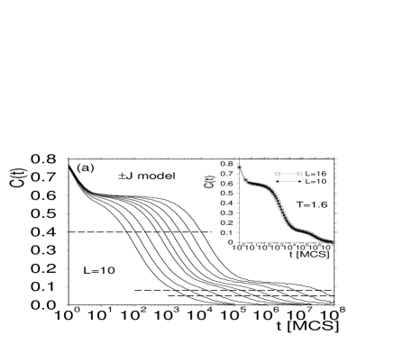
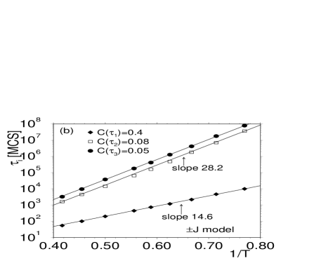
Figure 3: (a) Time dependence of the spin autocorrelation function $C(t)$ for temperatures (left to right) $T=2.4$, 2.2, 2.0, 1.8, 1.7, 1.6, 1.5, 1.4, and 1.3 ($L=10$). The horizontal dashed lines are used to define the relaxation times $\tau_{i}$ (see text for details). In the inset we compare $C(t)$ for $L=10$ and $L=16$ at $T=1.6$. (b) Symbols: Arrhenius plot of the relaxation time $\tau_{i}$ (see text for definition). Straight lines: Fits to the data with an Arrhenius law. The numbers are the activation energies.

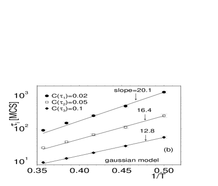
Figure 4: (a) Time dependence of the spin autocorrelation function $C(t)$ for temperatures $T=2.8$, 2.6, 2.4, 2.2, and 2.0 (left to right) for the Gaussian model. The horizontal dashed lines are used to define the relaxation times $\tau_{i}$ (see text for details). (b) Symbols: Arrhenius plot of the relaxation time $\tau_{i}$ (see text for definition). Straight lines: Fits to the data with an Arrhenius law. The numbers are the activation energies.

References

- (1) ELDERFIELD, D. and SHERRINGTON, D., J. Phys. C, 16 (1983) L497, L971, L1169.
- (2) GROSS, D. J., KANTER, I., and SOMPOLINSKY, H. Phys. Rev. Lett. 55 (1985) 304.
- (3) KIRKPATRICK, T. R. and WOLYNES, P. G., Phys. Rev. B 36 (1987) 8552; KIRKPATRICK, T.R. and THIRUMALAI, D., Phys. Rev. B 37 (1988) 5342; THIRUMALAI, D. and KIRKPATRICK, T. R., Phys. Rev. B 38 (1988) 4881.
- (4) CWILICH, G. and KIRKPATRICK, T. R., J. Phys. A: Math. Gen. 22 (1989) 4971; CWILICH, G., J. Phys. A: Math. Gen. 23 (1990) 5029.
- (5) CRISANTI, A., HORNER, H., and SOMMERS, H.-J., Z. Phys. B 92 (1993) 257.
- (6) DE SANTIS, E., PARISI, G., and RITORT, F., J. Phys. A: Math. Gen. 28 (1995) 3025.
- (7) KIRKPATRICK, T. R., and THIRUMALAI, D., Transp. Theory Stat. Phys. 24 (1995) 927.
- (8) DILLMANN, O., JANKE, W. and BINDER, K., J. Stat. Phys. 92 (1998) 57.
- (9) FRANZ, S. and PARISI, G., Physica A 261 (1998) 317; MEZARD, M. and PARISI, G., Phys. Rev. Lett. 82 (1999) 317; PARISI, G., Physica A 280 (2000) 115.
- (10) CRISANTI A. and RITORT F., Physica A 280 (2000) 155.
- (11) BRANGIAN, C., KOB, W., and BINDER, K., Europhys. Lett. 53 (2001) 756.
- (12) BRANGIAN, C., KOB, W., and BINDER, K., J. Phys. A: Math. Gen. 35 (2002) 191.
- (13) BRANGIAN, C. Dissertation (Johannes Gutenberg Universität, Mainz) (2002).
- (14) JÄCKLE, J., Rep. Progr. Phys. 49 (1986) 171.
- (15) GÖTZE, W. in Liquids, Freezing, and Glass Transition Eds.: Hansen, J. P., Levesque, D., and Zinn-Justin, J. (North-Holland, Amsterdam) 1990 p. 287.
- (16) GÖTZE, W., J. Phys.: Condens. Matter 11 (1999) A1.
- (17) KOB, W., J. Phys.: Condens. Matter 11 (1999) R85.
- (18) BINDER, K., J. Non-Cryst. Solids 274 (2000) 332.
- (19) BRANGIAN, C., KOB, W., and BINDER, K., Proceedings of the NATO ARW on “New Kinds of Phase Transitions in Disordered Materials” (in press).
- (20) LANDAU, D. P. and BINDER, K., A Guide to Monte Carlo Simulation in Statistical Physics (Cambridge Univ. Press, Cambridge) 2000.
- (21) WU F. Y., Rev. Mod. Phys. 54 (1982) 235; Rev. Mod. Phys. 55 (1982) 315; ZIA R. K. and WALLACE D. J., J. Phys. A: Math Gen. 8 (1975) 1495.
- (22) See, e.g., GARRAHAN J. P. and NEWMAN M. E. J., Phys. Rev. E 62 (2000) 7670.
- (23) STILLINGER F. H., J. Chem. Phys. 88, (1988) 7818.
- (24) KAUZMANN, W., Chem. Rev. 43 (1948) 219.
- (25) BINDER, K. and YOUNG, A. P., Rev. Mod. Phys. 58 (1986); YOUNG, A. P., Spin Glasses and Random Fields (World Scientific, Singapore) 1998.
- (26) SCHEUCHER, M. and REGER, J. D., Z. Phys. B 91 (1993) 383.
- (27) BINDER, K. and REGER, J. D., Adv. Phys. 41 (1992) 547.