Regular binary thermal lattice-gases

Abstract

We analyze the power spectrum of a regular binary thermal lattice gas in two dimensions and derive a Landau-Placzek formula, describing the power spectrum in the low-wavelength, low frequency domain, for both the full mixture and a single component in the binary mixture. The theoretical results are compared with simulations performed on this model and show a perfect agreement. The power spectrums are found to be similar in structure as the ones obtained for the continuous theory, in which the central peak is a complicated superposition of entropy and concentration contributions, due to the coupling of the fluctuations in these quantities. Spectra based on the relative difference between both components have in general additional Brillouin peaks as a consequence of the equipartition failure.

I Introduction

Lattice-gas automata (LGA), as introduced by Frisch, Hasslacher, and Pomeau Frisch et al. (1986), are ideal testing systems for kinetic theory. Although they have a simple structure, which makes them extremely efficient simulation tools, they still address the full many-body particle problem. Much of the efficiency originates from the discretization of the positions and velocities of the point-like particles onto a lattice. The simplified dynamics is a cyclic process: a streaming step, where all particles propagate to neighboring lattice sites, followed by a local collision step. The collisions typically conserve mass and momentum, and in addition energy if the model under consideration is thermal.

Lattice-gases are capable of simulating macroscopic fluid flow Frisch et al. (1986); Rivet and Boon (2001), and can be used for studying flow through porous media Chen et al. (1991), immiscible multicomponent fluids Gunstensen and Rothman (1991), reaction-diffusion Chopard et al. (1994), von Karman streets Malevanets and Kapral (1998), Rayleigh-Bénard convection Baran et al. (1997), interfaces and phase transitions Rothman (1994). However, there are practical problems when using LGA’s: the models are not Galilean-invariant, temperature is not well-defined, the transport coefficient have unexpected behavior as a function of temperature and density, and many models contain spurious invariants Brito et al. (1991); Das and Ernst (1992); Ernst and Das (1992). It is therefore difficult to make connections with realistic systems. Although in the early years the LGA’s were thought to seriously compete with other fluid flow solvers, the main line of research has shifted to a testing ground for concepts in kinetic theory. The main motivation for this paper lies in the exploration of the limits of thermal lattice-gas capabilities concerning diffusion-like phenomena.

Diffusion can be incorporated in LGA’s in several ways. The computational most efficient method is the color mixture Rivet and Boon (2001); Ernst and Dufty (1990); Hanon and Boon (1997), which we have analyzed in detail for a thermal model Blaak and Dubbeldam (2001a). The otherwise identical particles are in such a mixture painted with a probability corresponding to the concentration and a color-blind observer would not notice any difference, i.e. all transport properties are the same as for the single-component fluid. But in addition there is an extra hydrodynamical and color-dependent diffusion mode that does not interfere with the other modes.

In this paper we consider a different way to include diffusion, namely the regular binary mixture Ernst and Dufty (1990). In the regular binary mixture one has two distinct species of particles, i.e. different mass. For particles of the same species the exclusion principle holds and hence there can be at most one particle of a given species in any velocity channel. There is, however, no mutual exclusion for particles off different species. Consequently, a given velocity channel can be occupied by two particles, provided they both belong to a different species.

One can interpret this as each species living on its own but identical lattice with exclusion. Since each specie is restricted to its own lattice there can be no mass exchange between the two lattices and there is local mass conservation for both species. Upon interaction, however, particles of both lattices corresponding to the same node are able to exchange momentum and energy, provided this does no violate local mass conservation and exclusion for each species. Consequently, the dynamics of the regular binary mixture is much more involved than that of the color mixture, but it is closer to the dynamics of real fluids. For simplicity we here will assume the special case of the two species having the same physical properties, i.e. the same mass, and distinguish both species by a different color label.

We analyze the model at the microscopic level and focus mainly on the behavior of the power spectrum. The coupling between energy transport and diffusion that arises in these systems, results in a more complicated structure of the power spectrum Mountain and Deutch (1969); Boon and Yip (1980); Blaak and Dubbeldam (2001b), in which the central peak now contains combined effects of both entropy fluctuations and concentration fluctuations. Macroscopically this coupling manifests itself as the Dufour effect (a concentration gradient induces a heat-flow) and the Soret effect (a temperature gradient induces a diffusion flux).

The remainder of this paper is organized as follows. We start by introducing the regular binary thermal lattice gas model in section II and use the molecular chaos assumption to obtain the linearized collision operator. Section III is concerned with a mode analysis of the linearized system, revealing the appearance of an extra diffusion mode. The modes related to thermal diffusivity and mass-diffusion are coupled and form two non-propagating, diffusive modes. Furthermore, in section IV we derive a Landau-Placzek analogue, a formula which describes the power spectrum in the hydrodynamic limit (long wavelength, small frequency domain), which we check with simulation results performed on this system in section V. In the final section we give a brief overview of the main results and some concluding remarks.

II The regular binary GBL-model

The LGA model we like to consider here is a thermal model consisting of two different interacting species of particles with identical mass. They can be thought of to live on separate two-dimensional hexagonal lattices on which they propagate independently, but red and blue particles corresponding to the same node interact during the collision. The velocities are discretized and have a spatial layout as shown in figure 1. They are distributed over four rings: one ring contains a single null-velocity, and three rings each contain six velocities with magnitude $1$, $\sqrt{3}$, and $2$. The velocity set is of size $19$, and equivalent to the GBL-model, proposed by Grosfils, Boon, and Lallemand Grosfils et al. (1992). Since the model under consideration is basically a combination of two GBL models, particles of different type (red and blue) can have the same velocity. However, there can not be more than a single particle of each type in a given velocity state. The multiple rings correspond each to a different energy level and are a necessary requirement in order to introduce thermal properties. This particular velocity set guarantees the absence of spurious invariants and results in macroscopically isotropic behavior Grosfils et al. (1993).

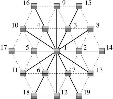
Figure 1: The spatial layout of the velocity set of the regular binary mixture. It is identical to the one for the GBL model, but now a channel can be occupied by a red, a blue or both at the same time.

The state of a node can be specified by a set of boolean occupation numbers $n_{i\mu}$, denoting the presence or absence of a particle of type $\mu=\{r,b\}$ in velocity channel $\bm{c}_{i}$, where $i$ is a label running over all 19 velocities. Due to the boolean nature of the LGA, the ensemble average of the occupation numbers $f_{i\mu}$ in equilibrium, is described by a Fermi-Dirac distribution Rivet and Boon (2001)

$$f_{i\mu}\equiv\langle n_{i\mu}\rangle=\frac{1}{1+e^{-\alpha_{\mu}+\frac{1}{2}\beta\bm{c}_{i}^{2}-\bm{\gamma}\cdot\bm{c}_{i}}},$$ (1)

where $\alpha_{r}$, $\alpha_{b}$, $\beta$, and $\bm{\gamma}$ are Lagrange multipliers and fixed by setting the value of the average red density $\rho_{r}=\sum_{ir}f_{ir}$, the average blue density $\rho_{b}=\sum_{ib}f_{ib}$ (or alternatively the total density $\rho=\rho_{r}+\rho_{b}$ and the fraction $P_{r}$ of red particles), the average velocity $\rho\bm{u}=\sum_{i\mu}f_{i\mu}\bm{c}_{i}$, and the energy density $\rho e=\frac{1}{2}\sum_{i\mu}f_{i\mu}\bm{c}_{i}^{2}$. Here, $\beta$ is the inverse temperature, $\alpha_{r}$ and $\alpha_{b}$ fulfill a chemical potential role, and $\bm{\gamma}$ is a parameter conjugate to the flow velocity. In the remainder of this paper we will restrict ourselves to the global zero-momentum case by putting $\bm{\gamma}=0$.

The lattice-gas Boltzmann equation, describing the time-evolution of the average occupation numbers, is given by Rivet and Boon (2001)

$$f_{i\mu}(\bm{r}+\bm{c}_{i},t+1)=f_{i\mu}(\bm{r},t)+\Delta_{i\mu}(f),$$ (2)

where the nonlinear collision term $\Delta_{i\mu}(f)$ is a summation over all pre-and post-collision states $s$ and $s^{\prime}$

$$\Delta_{i\mu}(f)=\sum_{s,s^{\prime}}P(s)A(s\rightarrow s^{\prime})(s_{i\mu}^{\prime}-s_{i\mu}).$$ (3)

The collision rules that are used are taken in to account by the transition matrix $A$, which contains the probability that on collision a state is transformed into an “equivalent” state. We denote the collection of states that can be transformed into each other by an equivalence class $\Gamma=(M_{r},M_{b},\bm{P},E)$, i.e. a class having the same red mass $M_{r}=\sum_{i}s_{ir}$, the same blue mass $M_{b}=\sum_{i}s_{ib}$, the same momentum $\bm{P}=\sum_{i\alpha}s_{i\alpha}\bm{c}_{i}$, and the same energy $E=\sum_{i\alpha}\frac{1}{2}s_{i\alpha}\bm{c}_{i}^{2}$. We adopt maximal collision rules, i.e. under collision a state can transform in any other state within the same equivalence class, including itself, thus fulfilling all conservation laws. Hence $A(\Gamma)=\frac{1}{|\Gamma|}$, where we use $|\Gamma|$ to denote the number of elements in the class $\Gamma$. The density and energy density enter the collision operator through $P(s)$, the probability of occurrence of state $s$ in equilibrium. In the Boltzmann approximation, the velocity channels are assumed to be independent, hence $P(s)$ can be written as

$$P(s)=\prod_{i\mu}f_{i\mu}^{s_{i\mu}}(1-f_{i\mu})^{1-s_{i\mu}}.$$ (4)

If the velocity fluctuations are sufficiently small a Taylor expansion of the collision term in the neighborhood of the equilibrium distribution is justified Rivet and Boon (2001), yielding the linearized collision operator $\Omega$

$$(\Omega\kappa)_{i\mu,j\nu}=\sum_{s,s^{\prime}}P(s)A(s\rightarrow s^{\prime})(s_{i\mu}^{\prime}-s_{i\mu})s_{j\nu},$$ (5)

where the diagonal matrix $\kappa_{i\mu,j\nu}$ is determined by $\kappa_{i\mu,i\mu}=f_{i\mu}(1-f_{i\mu})$, which is the variance in the occupation number of a channel with the corresponding labels. It can easily be checked from Eq. (5) that $\Omega\kappa$ is a symmetric $38\times 38$ matrix. In contrast with the colored LGA Blaak and Dubbeldam (2001a), $\kappa$ is a 38-dimensional diagonal matrix due to the fact that there is no mutual exclusion of a red and blue particle with the same velocity. It also enables us to introduce the colored thermal scalar product Hanon and Boon (1997); Blaak and Dubbeldam (2001a); Ernst and Das (1992),

$$\langle A|B\rangle =\sum_{i\mu}A(\bm{c}_{i\mu})B({\mathbf{c}}_{i\mu})\kappa_{i\mu},$$ (6)

$$\langle A|\Omega|B\rangle =\sum_{i\mu j\nu}A(\bm{c}_{i\mu})(\Omega\kappa)_{i\mu,j\nu}B(\bm{c}_{j\nu}),$$ (7)

where we adopt the convention that the matrix $\kappa$ is attached to the right vector.

III Perturbation theory

In first approximation the behavior of the system can be obtained by considering the fluctuations $\delta f_{i\nu}(\bm{r},t)=f_{i\nu}(\bm{r},t)-f_{i\nu}$ and analyze these deviations from the uniform equilibrium state in terms of eigenmodes. The solutions of the Boltzmann equation (2) are then of the form

$$\delta f_{i\nu}=\psi_{\mu}(\bm{k,c_{i}})e^{-\imath\bm{k}\cdot\bm{r}+z_{\mu}(\bm{k})t},$$ (8)

where $z_{\mu}(\bm{k})$ represents the eigenvalue of the mode $\psi_{\mu}$ at wavevector $\bm{k}$. The hydrodynamic modes are related to the collisional invariants and satisfy $z_{\mu}\rightarrow 0$ for $\bm{k}\rightarrow 0$. There are five independent collision invariants $a_{n}$ corresponding to the conservation of the red and blue mass, the conservation of momentum, and the conservation of energy

$$\langle a_{n}|\Omega=0\qquad\Omega|a_{n}\rangle=0,$$ (9)

$$|a_{n}\rangle=\{|R\rangle,|B\rangle,|c_{x}\rangle,|c_{y}\rangle,|\frac{1}{2}c^{2}\rangle\},$$ (10)

where $|R\rangle_{i\alpha}=\delta_{\alpha r}$, $|B\rangle_{i\alpha}=\delta_{\alpha b}$, and can be combined to form $|\rho\rangle=|R\rangle+|B\rangle$. It turns out that an equivalent and more convenient set of invariants is given by the following five combinations which are mutual orthogonal with respect to the colored thermal scalar product (6)

$$|a_{n}\rangle=\{|c_{x}\rangle,|c_{y}\rangle,|p\rangle=|\frac{1}{2}c^{2}\rangle,|s\rangle=|p\rangle-c_{s}^{2}|\rho\rangle,|d\rangle\},$$ (11)

where $|s\rangle$ is the analogue to the microscopic entropy for the GBL model Grosfils et al. (1993) and $c_{s}^{2}=\frac{\langle p|p\rangle}{\langle p|\rho\rangle}$ the speed of sound following from the orthogonality requirement $\langle p|s\rangle=0$. The remaining invariant $|d\rangle$ is, contrary to the one in the colored GBL model Blaak and Dubbeldam (2001a), not simply the weighted difference between the red and blue densities $\frac{1}{\langle R|R\rangle}|R\rangle-\frac{1}{\langle B|B\rangle}|B\rangle$, but is given by

$$|d\rangle=\left(\frac{|R\rangle}{\langle s|R\rangle}-\frac{|B\rangle}{\langle s|B\rangle}\right)-\left(\frac{\langle p|R\rangle}{\langle s|R\rangle}-\frac{\langle p|B\rangle}{\langle s|B\rangle}\right)\frac{|p\rangle}{\langle p|p\rangle}.$$ (12)

This form is determined by the requirement that it is orthogonal to the four other invariants. In the case of equal red and blue density the last term on the righthand side vanishes, but in general this is not the case. The origin of this term is in fact the absence of equipartition in this model due to the exclusion principle, which causes the ratio $f_{ir}/f_{ib}$ to be dependent on the velocity of the particles as can be seen from Eq. (1). Note that this last invariant is also perpendicular to the density, i.e. $\langle\rho|d\rangle=0$. Other useful relations between these invariants are $\langle\rho|p\rangle=\langle\rho|c_{x}^{2}\rangle=\langle\rho|c_{y}^{2}\rangle$ and $\langle p|p\rangle=\langle p|c_{x}^{2}\rangle=\langle p|c_{y}^{2}\rangle$.

The choice of $|s\rangle$ and $|d\rangle$ made here is based on the correspondence of the definition of $|s\rangle$ with the one made for the GBL model and its colored counterpart Blaak and Dubbeldam (2001a); Grosfils et al. (1993). Since $|s\rangle$ nor $|d\rangle$, with the exception of some special limits, is going to be the zeroth order of an eigenmode the choice is somewhat arbitrary and any two linear combinations that are mutual orthogonal could be used as well. The current choice, however, will facilitate us to make a connection with continuous theory and the proper transport coefficients.

Note that this is similar to what is done in the case of continuous theory and generalized versions of hydrodynamics (See Ref. Boon and Yip (1980) and references therein), where one also needs to obtain a set of variables that are statistically independent based on thermodynamic fluctuation theory. This does not uniquely fix these variables, and the freedom that remains can be used in order to select an appropriate, orthogonal set for the specific problem.

Following the method of Résibois and Leener Résibois and de Leener (1977) we need to find the $\bm{k}$-dependent eigenfunctions and eigenvalues of the single-time step Boltzmann propagator

$$e^{-\imath\bm{k}\cdot\bm{c}}(\bm{1}+\Omega)|\psi(\bm{k})\rangle=e^{z(\bm{k})}|\psi(\bm{k})\rangle,$$ (13)

$$\langle\phi(\bm{k})|e^{-\imath\bm{k}\cdot\bm{c}}(\bm{1}+\Omega)=e^{z(\bm{k})}\langle\phi(\bm{k})|,$$ (14)

where $e^{-\imath\bm{k}\cdot\bm{c}}$ has to be interpreted as a diagonal matrix, and $\bm{1}$ is the identity matrix. The symmetries of the matrices cause the left and right eigenvectors to be related by $\phi_{\mu}({\bf k})=e^{\imath\bm{k}\cdot\bm{c}}\psi_{\mu}({\bf k})/{\cal M}_{\mu}$, and form a complete biorthonormal set

$$\sum_{\mu}|\psi_{\mu}\rangle\langle\phi_{\mu}|=\bm{1}\qquad\langle\phi_{\mu}|\psi_{\nu}\rangle=\delta_{\mu\nu},$$ (15)

where we used $\mu$ and $\nu$ to label the different eigenfunctions and introduced the normalization constants ${\cal M}_{\mu}$.

To obtain the hydrodynamic modes characterized by $z(\bm{k})\rightarrow 0$ in the limit $\bm{k}\rightarrow 0$, we make a Taylor expansion of the eigenfunctions and eigenvalues

$$\psi_{\mu}(\bm{k})=\psi_{\mu}^{(0)}+(\imath k)\psi_{\mu}^{(1)}+(\imath k)^{2}\psi_{\mu}^{(2)}+\cdots,$$ (16)

$$z_{\mu}(\bm{k})=(\imath k)z_{\mu}^{(1)}+(\imath k)^{2}z_{\mu}^{(2)}+\cdots,$$ (17)

where we already used that $z_{\mu}^{(0)}=0$. The functions $\psi_{\mu}(\bm{k})$ will be determined up to a normalization factor. As this normalization is not allowed to be observable, and in fact will not be observable, we can choose it in a convenient way by

$$\langle\psi_{\mu}^{(0)}|\psi_{\mu}(\bm{k})\rangle=\langle\psi_{\mu}^{(0)}|\psi_{\mu}^{(0)}\rangle,$$ (18)

which leads to

$$\langle\psi_{\mu}^{(0)}|\psi_{\mu}^{(n)}\rangle=\delta_{n0}\langle\psi_{\mu}^{(0)}|\psi_{\mu}^{(0)}\rangle.$$ (19)

Substitution of the expansions in Eq. (13) and grouping according to the same order in $k$ gives

$$\Omega|\psi_{\mu}^{(0)}\rangle=0,$$ (20)

$$\Omega|\psi_{\mu}^{(1)}\rangle=(c_{\ell}+z_{\mu}^{(1)})|\psi_{\mu}^{(0)}\rangle,$$ (21)

$$\Omega|\psi_{\mu}^{(2)}\rangle=(c_{\ell}+z_{\mu}^{(1)})|\psi_{\mu}^{(1)}\rangle+\left[z_{\mu}^{(2)}+\frac{1}{2}(c_{\ell}+z_{\mu}^{(1)})^{2}\right]|\psi_{\mu}^{(0)}\rangle,$$ (22)

with $c_{\ell}=\hat{\bm{k}}\cdot\bm{c}$ and its orthogonal counterpart $c_{\perp}=\hat{\bm{k}}_{\perp}\cdot\bm{c}$.

The solution of the zeroth order equation is straightforward and gives

$$|\psi_{\mu}^{(0)}\rangle=\sum_{n}A_{\mu n}|a_{n}\rangle,$$ (23)

with some unknown coefficients $A_{\mu n}$. Substitution in the first order equation and multiplying with $\langle a_{m}|$ at the left gives for each $m$ a linear equation in the $A_{\mu n}$

$$\sum_{n}A_{\mu n}\langle a_{m}|c_{\ell}+z_{\mu}^{(1)}|a_{n}\rangle=0,$$ (24)

where we used that $\langle a_{m}|\Omega=0$. This set of equations has a solution provided the determinant is zero, leading to the following eigenvalue equation for $z_{\mu}^{(1)}$

$$\left(z_{\mu}^{(1)}\right)^{3}\left(\langle p|p\rangle\langle c_{\ell}|c_{\ell}\rangle\left(z_{\mu}^{(1)}\right)^{2}-\langle p|c_{\ell}\rangle^{2}\right)=0,$$ (25)

where it is used that combinations containing an odd power of $c_{\ell}$ or $c_{\perp}$ are necessarily zero. This determines two of the five zeroth order eigenfunctions

$$|\psi_{\sigma}^{(0)}\rangle=|p\rangle+\sigma c_{s}|c_{\ell}\rangle\qquad z_{\pm}^{(1)}=-\sigma c_{s},$$ (26)

where $\sigma=\pm$ denotes opposite directions parallel to $\bm{k}$ and

$$\left(z_{\sigma}^{(1)}\right)^{2}=\frac{\langle p|c_{\ell}^{2}\rangle^{2}}{\langle p|p\rangle\langle p|\rho\rangle}=c_{s}^{2}.$$ (27)

For the remaining three eigenfunctions we can only conclude at this level that they satisfy $z_{\mu}^{(1)}=0$ and are formed by combinations of $|d\rangle$, $|s\rangle$, and $|c_{\perp}\rangle$ only. On physical grounds it can be argued that $|c_{\perp}\rangle$ will be a mode on itself, however, it also will follow in a natural way later on.

The combination $|j_{\mu}\rangle=c_{\ell}+z_{\mu}^{(1)}|\psi_{\mu}^{(0)}\rangle$ is called the current. We will extend the definitions of the current $j_{\mu}$ and $\psi_{\mu}^{(0)}$ to include $s$ and $d$ as a possible value for $\mu$. This is for convenience, since strictly speaking $|s\rangle$ and $|d\rangle$ will in general not be the source of an eigenfunction, but both will be a linear combination of two “true” modes of the system.

With the introduction of these currents it follows immediately from Eqns. (9) and (21) that invariants and currents are orthogonal

$$\langle\psi_{\nu}^{(0)}|j_{\mu}\rangle=0,$$ (28)

hence the currents lie in the complement of the null-space. Since this is not affected by applying $\Omega$ we obtain

$$\langle\psi_{\nu}^{(0)}|\Omega^{m}|j_{\mu}\rangle=0$$ (29)

for any integer $m$, including negative values. Note that for negative values of $m$ the expression $\Omega^{m}|j_{\mu}\rangle$ is uniquely determined by the requirement that the result has no component in the null-space. Therefore the solution of the first order equation (21) can formally be written as

$$|\psi_{\mu}^{(1)}\rangle=\frac{1}{\Omega}|j_{\mu}\rangle+\sum_{\nu}B_{\mu\nu}|\psi_{\nu}^{(0)}\rangle,$$ (30)

with yet to be determined coefficients $B_{\mu\nu}$ and also three still unknown currents. The coefficients $B_{\mu\mu}=0$ as follows from the chosen normalization (19) of the eigenfunctions.

Multiplying the second order equation (22) with $\langle\psi_{\lambda}^{(0)}|$ at the left side we find

$$0= \langle\psi_{\lambda}^{(0)}|(c_{\ell}+z_{\lambda}^{(1)})|\psi_{\mu}^{(1)}\rangle+(z_{\mu}^{(1)}-z_{\lambda}^{(1)})\langle\psi_{\lambda}^{(0)}|\psi_{\mu}^{(1)}\rangle+$$ (31)

$$z_{\mu}^{(2)}\langle\psi_{\lambda}^{(0)}|\psi_{\mu}^{(0)}\rangle+\frac{1}{2}\langle\psi_{\lambda}^{(0)}|(c_{\ell}+z_{\lambda}^{(1)})(c_{\ell}+z_{\mu}^{(1)})|\psi_{\mu}^{(0)}\rangle+$$

$$\frac{1}{2}(z_{\mu}^{(1)}-z_{\lambda}^{(1)})\langle\psi_{\lambda}^{(0)}|(c_{\ell}+z_{\mu}^{(1)})|\psi_{\mu}^{(0)}\rangle.$$

Using the definition of the currents, substitution of the formal solution of the first order equation (30), and using the orthogonality relations (28) this leads to

$$z_{\mu}^{(2)}\langle\psi_{\lambda}^{(0)}|\psi_{\mu}^{(0)}\rangle+(z_{\mu}^{(1)}-z_{\lambda}^{(1)})B_{\mu\lambda}\langle\psi_{\lambda}^{(0)}|\psi_{\lambda}^{(0)}\rangle=-\langle j_{\lambda}|\frac{1}{\Omega}+\frac{1}{2}|j_{\mu}\rangle.$$ (32)

For $\lambda=\mu$ this gives the five transport coefficients

$$z_{\mu}^{(2)}=-\frac{\langle j_{\mu}|\frac{1}{\Omega}+\frac{1}{2}|j_{\mu}\rangle}{\langle\psi_{\mu}^{(0)}|\psi_{\mu}^{(0)}\rangle},$$ (33)

and for $\lambda\neq\mu$

$$(z_{\mu}^{(1)}-z_{\lambda}^{(1)})B_{\mu\lambda}\langle\psi_{\lambda}^{(0)}|\psi_{\lambda}^{(0)}\rangle=-\langle j_{\lambda}|\frac{1}{\Omega}+\frac{1}{2}|j_{\mu}\rangle,$$ (34)

from which some of the values of $B_{\mu\lambda}$ can be obtained, provided that $(z_{\mu}^{(1)}-z_{\lambda}^{(1)})$ is nonzero, and of which the resulting expressions can be found in Appendix A. Note that at this stage three of the zeroth order eigenfunctions and their corresponding currents are still undetermined.

In the space of $|d\rangle$, $|s\rangle$, and $|c_{\perp}\rangle$ one can rewrite Eq. (32) in the form of a new eigenvalue problem in the still undetermined coefficients $A_{\mu n}$

$$\sum_{n}\left(\langle j_{m}|\frac{1}{\Omega}+\frac{1}{2}|j_{n}\rangle+z_{\mu}^{(2)}\langle a_{m}|a_{n}\rangle\right)A_{\mu n}=0.$$ (35)

Equating the determinant to zero we find that there are three different eigenvalues and we can obtain the form of the remaining three zeroth order eigenfunctions. Using the fact that there is no degeneracy we know that we can diagonalize the matrix in terms of the proper functions. Hence the off-diagonal matrix elements $\langle j_{\mu}|\frac{1}{\Omega}+\frac{1}{2}|j_{\nu}\rangle$ need to vanish, which could already be seen from Eq. (34) since for these modes we have $z_{\mu}^{(1)}=0$. It can also easily be checked from symmetry considerations that $|c_{\perp}\rangle$ is one of the modes as was suggested earlier. The solution of the remaining two zeroth order eigenfunctions is straightforward and leads to

$$|\psi_{\perp}^{(0)}\rangle =|c_{\perp}\rangle,$$ (36)

$$|\psi_{s_{\pm}}^{(0)}\rangle =|s_{\pm}\rangle=\frac{|s\rangle}{\sqrt{\langle s|s\rangle}}+\left(-\xi\pm\sqrt{1+\xi^{2}}\right)\frac{|d\rangle}{\sqrt{\langle d|d\rangle}},$$ (37)

where the prefactors are determined by the requirements

$$\langle s_{\pm}|s_{\mp}\rangle =0,$$ (38)

$$\langle j_{s_{\pm}}|\frac{1}{\Omega}+\frac{1}{2}|j_{s_{\mp}}\rangle =0,$$ (39)

and we have introduced the short hand notation

$$\xi\equiv\frac{\chi-{\mathcal{D}}}{2Q},$$ (40)

with

$$\chi \equiv-\frac{\langle j_{s}|\frac{1}{\Omega}+\frac{1}{2}|j_{s}\rangle}{\langle s|s\rangle},$$ (41)

$${\cal D} \equiv-\frac{\langle j_{d}|\frac{1}{\Omega}+\frac{1}{2}|j_{d}\rangle}{\langle d|d\rangle},$$ (42)

$$Q \equiv-\frac{\langle j_{s}|\frac{1}{\Omega}+\frac{1}{2}|j_{d}\rangle}{\sqrt{\langle s|s\rangle\langle d|d\rangle}}.$$ (43)

As the form of the last three quantities suggests by comparison with Eq. (33), these quantities are related to transport coefficients. In the low density limit and in the limit of only one specie, one can identify $\chi$ as being the thermal diffusivity of the GBL model. In the low density limit ${\cal D}$ will correspond to the self-diffusion coefficient. Their interpretation as transport coefficients is justified in Appendix B. The remaining value $Q$ can not be interpreted as a transport value, but rather is some measure of the coupling between different modes.

Using Eq. (33) we can evaluate the five transport coefficients corresponding to the hydrodynamic modes. In the case of the two soundmodes (26) this leads to the sounddamping $\Gamma$

$$z_{\pm}^{(2)}=\Gamma=-\frac{\langle j_{\pm}|\frac{1}{\Omega}+\frac{1}{2}|j_{\pm}\rangle}{\langle\psi_{\pm}^{(0)}|\psi_{\pm}^{(0)}\rangle},$$ (44)

while the perpendicular mode (36) gives rise to the viscosity $\nu$

$$z_{\perp}^{(2)}=\nu=-\frac{\langle j_{\perp}|\frac{1}{\Omega}+\frac{1}{2}|j_{\perp}\rangle}{\langle c_{\perp}|c_{\perp}\rangle}.$$ (45)

By writing out the definitions of $|s_{\pm}\rangle$ and $|j_{s_{\pm}}\rangle$ and using the introduced quantities (40) - (43) where needed, we can rewrite the second order eigenvalues of the two non-propagating modes $|s_{\pm}\rangle$ as

$$s^{\circ}_{\pm}=-\frac{\langle j_{s_{\pm}}|\frac{1}{\Omega}+\frac{1}{2}|j_{s_{\pm}}\rangle}{\langle s_{\pm}|s_{\pm}\rangle}=\frac{1}{2}(\chi+{\cal D})\pm Q\sqrt{1+\frac{(\chi-{\cal D})^{2}}{4Q^{2}}}.$$ (46)

In the low density limit one finds that the two eigenmodes (37) up to a normalization factor will converge to $|s\rangle$ and $|d\rangle$ as defined in Eqns. (11) and (12). Consequently one obtains $s^{\circ}_{\pm}\rightarrow\chi,{\cal D}$, which is an illustration of the decoupling of entropy and concentration fluctuations in this limit. In general, however, these two “true” transport coefficients do not seem to correspond with a conventional transport coefficient, but rather they always appear in combination with each other, and it is only in the appropriate limits that they reduce to the thermal diffusivity and diffusion coefficient. This is completely in agreement with the results known for the continuous theory Boon and Yip (1980), where the coupling of fluctuations in concentration and entropy results in the same effect.

In the present model, however, there is some ambiguity in the choice made for the basic invariants. To arrive at this last formula it was only necessary to assume that the invariants $|s\rangle$ and $|d\rangle$, are mutually orthogonal, and span a 2-dimensional subspace in the null-space which is perpendicular to $|c_{\ell}\rangle$, $|c_{\perp}\rangle$, and $|p\rangle$. A good choice necessarily leads to the proper modes in the fully known limit of one specie. Although this puts some limitations on the possible choices it will not uniquely fix the basis. The present choice for $|s\rangle$ in (11) is however the most natural extension of the conventional formulation Grosfils et al. (1993) and we will refer to $\chi$ as being the generalized thermal diffusivity.

This problem is more easily identified in the diffusion-like mode $|d\rangle$. In the present formulation (12), it contains in general a contribution proportional to $|p\rangle$, rather than being a weighted difference of the red and blue densities only as found in the colored GBL model Blaak and Dubbeldam (2001a). This already suggests that this vector is not the proper generalization of the self-diffusion mode. This is consistent with the continuous theory Boon and Yip (1980), where the analogue of the $s_{\pm}^{\circ}$ also depend on more than the thermal diffusivity and diffusion only. We will address this subject again in a later section.

Similar to the case of the GBL model we can introduce $\gamma$, the ratio of specific heats by

$$\gamma=1+\frac{\langle s|s\rangle}{\langle p|p\rangle}=\frac{\langle p|p\rangle\langle\rho|\rho\rangle}{\langle p|\rho\rangle^{2}}=\frac{c_{s}^{2}}{c_{T}^{2}},$$ (47)

with $c_{s}^{2}=\langle p|p\rangle/\langle p|\rho\rangle$ the adiabatic speed of sound, $c_{T}^{2}=\langle p|\rho\rangle/\langle\rho|\rho\rangle$ the isothermal speed of sound. Two additional useful definitions are $\tau_{xy}=c_{\ell}c_{\perp}$ and $\tau_{xx}=\frac{1}{2}(c_{\ell}^{2}-c_{\perp}^{2})$. These allow us to rewrite the currents related to the sound modes as $|j_{\pm}\rangle=|j_{s}\rangle\pm c_{s}|\tau_{xx}\rangle$. Consequently this leads to

$$\Gamma=-\frac{\langle j_{s}|\frac{1}{\Omega}+\frac{1}{2}|j_{s}\rangle+c_{s}^{2}\langle\tau_{xx}|\frac{1}{\Omega}+\frac{1}{2}|\tau_{xx}\rangle\pm 2c_{s}^{2}\langle j_{s}|\frac{1}{\Omega}+\frac{1}{2}|\tau_{xx}\rangle}{\langle p|p\rangle+c_{s}^{2}\langle c_{\ell}|c_{\ell}\rangle\pm 2c_{s}\langle p|c_{\ell}\rangle}.$$ (48)

From symmetry considerations it follows that $\langle p|c_{\ell}\rangle=0$ and $\langle j_{s}|\frac{1}{\Omega}+\frac{1}{2}|\tau_{xx}\rangle=0$, and since $\langle\tau_{xx}|\frac{1}{\Omega}+\frac{1}{2}|\tau_{xx}\rangle=\langle\tau_{xy}|\frac{1}{\Omega}+\frac{1}{2}|\tau_{xy}\rangle$ because of the isotropy of the lattice, we obtain the following relation for the main transport coefficients

$$\Gamma=\frac{1}{2}\left(\nu+(\gamma-1)\chi\right).$$ (49)

Figure 2: The real part of the full eigenvalue spectrum as a function of the wavevector $|\bm{k}|$ in reciprocal lattice units. The system parameters are $\rho=6.0$, $e=1.0$, and $P_{r}=0.75$. Note that there are five hydrodynamic modes in the small wavevector limit. Two of them, related to the soundmodes, coincide.

An example of the full wave-vector dependent real eigenvalue spectrum is shown in Fig. 2, which also confirms the absence of spurious invariants. Of all eigenvalues only the five related to the hydrodynamic modes go to zero in the limit $\bm{k}\rightarrow 0$. It is with these modes that the binary-mixture responds to deviations from thermal equilibrium

$$z_{\pm}(\bm{k}) =-\pm\imath c_{s}\bm{k}-\Gamma\bm{k}^{2},$$ (50)

$$z_{\perp}(\bm{k}) =-\nu\bm{k}^{2},$$ (51)

$$z_{s_{\pm}}(\bm{k}) =-s^{\circ}_{\pm}\bm{k}^{2}.$$ (52)

The first two eigenvalues describe sound propagation in the two opposite directions parallel to $\bm{k}$ with $c_{s}$ the adiabatic sound speed, the third eigenvalue describes the shear mode, and the last two eigenvalues represent purely diffusive, non-propagating processes. In this hydrodynamic regime characterized by $k\lambda\ll 1$, where $\lambda$ is the mean free path length, one can exploit the fact that the real component of the eigenvalues of the hydrodynamic modes is much smaller than that of the kinetic modes. We will use this in the next section in order to obtain the Landau-Placzek formula (59) for the power spectrum.

For larger wavevectors (here roughly $0.5\leq k\leq 1.5$) the relations (50)-(52) start to deviate from the true values. This is the generalized hydrodynamic regime ($k\lambda\lesssim 1$), and the transport coefficients become $k$ dependent. The hydrodynamic modes are, however, still smaller than the kinetic modes yielding a reasonable accurate Landau-Placzek formula. In the kinetic regime ($k\lambda\gtrsim 1$) the hydrodynamic modes and kinetic modes become of the same order of magnitude. The distinction between fast and slow modes can not be made and all modes contribute to the power spectrum.

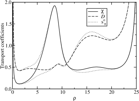
Figure 3: The “true” transport values $s^{\circ}_{\pm}$, and the transport coefficients $\chi$, ${\cal D}$ as a function of the density at $\theta=0.05$ and $P_{r}=0.75$. In the low density limit, and by the duality of the model also in the high density limit, the two sets converge.

In Fig. 3 the diffusive transport properties are shown at fixed reduced temperature $\theta=\exp(-\frac{1}{2}\beta)$. The modes $s^{\circ}_{\pm}$ are the modes observed in the eigenvalue spectrum and are combinations of $\chi$, ${\cal D}$, and $Q$. In the low density limit these two modes converge to the thermal diffusivity and diffusion, i.e. $s^{\circ}_{+}\rightarrow\chi$, $s^{\circ}_{-}\rightarrow{\cal D}$, and is caused by the decoupling of the fluctuations in the concentrations and entropy. In our model this means that the ratio $Q/(\chi-{\cal D})$ vanishes. The value of $Q$, however, will in general remain small but finite due to the divergencies of the transport coefficients in the low density limit of LGA. The same is observed in the high density limit, which is merely an illustration of the duality of the LGA-model if one interchanges particles and holes. In both cases this is a direct consequence of the fact that the fluctuations in the occupation numbers become linear in the average occupation densities, thus leading to equipartition.

As an additional remark we like to mention that the value of $Q$ can be both positive and negative. Therefore the correct curves of $s_{\pm}^{\circ}$ need not be continuous as a function of the density, but can contain discontinuities located at points where $Q$ changes sign. Consequently, depending on the system parameters, the role of $s^{\circ}_{+}$ and $s^{\circ}_{-}$ is interchanged with respect to $\chi$ and ${\cal D}$. This is merely due to the choice in convention we have used in Eq. (37) and of no physical importance.

For some intermediate values of the density one also finds that the values of $s^{\circ}_{\pm}$ and $\chi,{\cal D}$ coincide. This is, however, not caused by decoupling of the fluctuations. In these cases there is no effective equipartition, but one obtains $Q=0$ as a consequence of the cancellation of terms. Moreover, the location of these points depends in a non-trivial way on the system parameters.

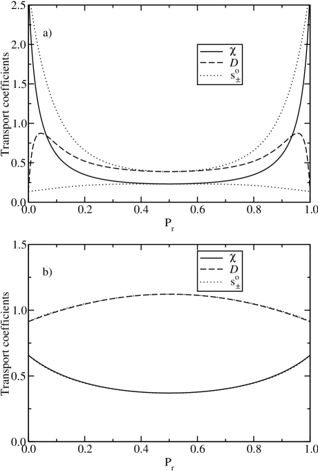
Figure 4: The transport coefficients as a function of $P_{r}$ at (a) $\rho=4$, $\theta=0.05$ and (b) $\rho=0.25$, $\theta=0.05$. For low densities decoupling occurs for any composition, for higher densities only in the limits $P_{r}=1$ and $P_{r}=1/2$.

The diffusive transport properties versus the relative concentration of both species at fixed density and reduced temperature $\theta$ is shown in Fig. 4. In the low density limit we have $s_{\pm}^{\circ}\rightarrow\chi,{\cal D}$ for all relative concentrations. This is not generally true as can be seen from the higher density figure. It does, however, reveal that the decoupling also occurs in general for the single specie limits $P_{r}\rightarrow 0$ and $P_{r}\rightarrow 1$. This is not surprising, as in those limits the model effectively reduces to a normal GBL model with only a single diffusive mode related to the thermal diffusivity. This is actually also the case in the high density limit of Fig. 3, because there one has a situation in which the red lattice is almost completely filled and therefore an effective blue system that remains.

Finally, decoupling can also be observed in the case $P_{r}=P_{b}$. In fact this is a rather special limit and could be analyzed completely in a manner similar to the one used for the colored GBL model Blaak and Dubbeldam (2001a), because based on the symmetry of the problem one can decompose the linearized Boltzmann operator in two type of contributions, i.e. $|R\rangle+|B\rangle$ and $|R\rangle-|B\rangle$.

For $P_{r}=0$ the diffusion mode vanishes, since we then recover the original GBL model, but for $P_{r}\rightarrow 0$ the diffusion mode remains finite. This case is illustrated in Fig. 5. Here, in the low density limit the diffusion mode becomes equal to the self-diffusion of the GBL model (and hence also equal to the diffusion mode in the GBL color mixture), but for higher density they deviate. A behavior that finds its origin in the fact that the color mixture does not allow more than one particle in a single velocity channel and, although the number of particles of the second specie gets very small, they still have a large impact on the diffusion.

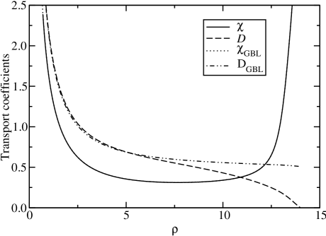
Figure 5: A comparison of the transport coefficients of the present model in the limit $P_{r}\rightarrow 1$ with those of the GBL model for fixed average energy density $e=1.0$. $\chi$ coincides with the thermal diffusivity $\chi_{\text{GBL}}$ of the GBL model, ${\cal D}$ matches the self-diffusion $D_{\text{GBL}}$ only for the lower densities. The values of $s^{\circ}_{\pm}$ are not shown but overlap completely with $\chi$ and ${\cal D}$.

IV Landau-Placzek theory

IV.1 Full spectrum

In the hydrodynamic regime of small wavevectors ($k\rightarrow 0$) and the frequency $\omega$ being linear in $k$, the spectral density $S(\bm{k},\omega)$ can be expanded in powers of $\imath k$. In this long-wavelength, small frequency limit the hydrodynamic modes are well separated from the kinetic modes, which can be neglected due to their exponential decay. By keeping only terms up to $\bm{O}(k^{2})$ ($\omega/k$ is kept constant for consistency), one obtains the Landau-Placzek approximation.

It has been shown that the dynamic structure factor can be evaluated by Grosfils et al. (1993)

$$\frac{S(\bm{k},\omega)}{S(\bm{k})}=2\text{Re}\frac{\langle\rho|(e^{\imath\omega+\imath\bm{k}\cdot\bm{c}}-1-\Omega)^{-1}+\frac{1}{2}|\rho\rangle}{\langle\rho|\rho\rangle}.$$ (53)

The closely related spectral function $F(\bm{k},\omega)$ can be written as

$$F(\bm{k},\omega)\equiv\langle\rho|(e^{\imath\omega+\imath\bm{k}\cdot\bm{c}}-1-\Omega)^{-1}+\frac{1}{2}|\rho\rangle=2\sum_{\mu}\text{Re}{\cal N}_{\mu}{\cal D}_{\mu},$$ (54)

where

$${\cal D}_{\mu} =\frac{1}{e^{\imath w-z_{\mu}}-1}+\frac{1}{2}\approx\frac{z_{\mu}^{(2)}-\imath(w-z_{\mu}^{(1)}k)}{(z_{\mu}^{(2)}k^{2})^{2}+(w-z_{\mu}^{(1)}k)^{2}},$$ (55)

$${\cal N}_{\mu} =\langle\rho|\psi_{\mu}\rangle\langle\phi_{\mu}|\rho\rangle.$$ (56)

The coefficients ${\cal N}_{\mu}$ are evaluated in Appendix A for small $\bm{k}$ and yield

$${\cal N}_{\sigma} =\frac{\langle\rho|\rho\rangle}{2\gamma}\left(1+\frac{\imath\sigma k}{c_{s}}\left[\Gamma+(\gamma-1)\chi\right]\right),$$ (57)

$${\cal N}_{s_{\pm}} =\frac{(\gamma-1)\langle\rho|\rho\rangle}{2\gamma}\left(1\pm\frac{\chi-{\cal D}}{s^{\circ}_{+}-s^{\circ}_{-}}\right).$$ (58)

From symmetry considerations one can conclude that the shear mode will not contribute to the spectrum and one finds ${\cal N}_{\perp}=0$. Combining these results with the expressions (54) and (55), we finally obtain the Landau-Placzek formula, describing the power-spectrum in the hydrodynamical domain

$$\frac{S(\bm{k},\omega)}{S(\bm{k})}=\frac{\gamma-1}{\gamma}\left[\left(1+\frac{\chi-{\cal D}}{s^{\circ}_{+}-s^{\circ}_{-}}\right)\frac{s^{\circ}_{+}k^{2}}{\omega^{2}+(s^{\circ}_{+}k^{2})^{2}}+\left(1-\frac{\chi-{\cal D}}{s^{\circ}_{+}-s^{\circ}_{-}}\right)\frac{s^{\circ}_{-}k^{2}}{\omega^{2}+(s^{\circ}_{-}k^{2})^{2}}\right]$$

$$+\frac{1}{\gamma}\left[\frac{\Gamma k^{2}}{(\omega+c_{s}k)^{2}+(\Gamma k^{2})^{2}}+\frac{\Gamma k^{2}}{(\omega-c_{s}k)^{2}+(\Gamma k^{2})^{2}}\right]$$

$$+\frac{1}{\gamma}\left[\Gamma+(\gamma-1)\chi\right]\frac{k}{c_{s}}\left[\frac{\omega+c_{s}k}{(\omega+c_{s}k)^{2}+(\Gamma k^{2})^{2}}-\frac{\omega-c_{s}k}{(\omega-c_{s}k)^{2}+(\Gamma k^{2})^{2}}\right].$$ (59)

The spectrum contains an unshifted central peak that is formed by two Lorentzians due to the two processes related to the non-propagating modes $s_{\pm}^{\circ}$. The two propagating modes lead to the presence of the two shifted Brillouin lines. Their width at half-height can be used as a measurement of $\Gamma\bm{k}^{2}$, the position of the peaks can be used a measurement of $\pm c_{s}\bm{k}$. The last two terms in Eq. (59) give an asymmetric correction to the Brillouin peaks and induce a slight pulling of the peaks toward the central peak.

The symmetry of the different contributions is such that the ratio of the integrated contributions of the central peak and the Brillouin components is constant and given by

$$\frac{\sum_{\sigma}\int d\omega Re({\cal N}_{s_{\sigma}}{\cal D}_{s_{\sigma}})}{\sum_{\sigma}\int d\omega Re({\cal N}_{\sigma}{\cal D}_{\sigma})}=\gamma-1.$$ (60)

Figure 6: Boltzmann spectra and Landau-Placzek approximations for the full (a,c) and for the red spectrum (b,d). The system parameters are $\rho=10$, $P_{r}=0.25$, $e=0.75$, $k_{x}=10\times 2\pi/512$ (a,b) and $\rho=1$, $P_{r}=0.35$, $e=1.0$, $k_{x}=52\times 2\pi/512$ (c,d). The solid and dotted curves are the Boltzmann results and Landau-Placzek approximations respectively. Simulations results are indicated by the points. The wavevector $\bm{k}$ is given in reciprocal lattice units, the frequency $\omega$ in reciprocal time ($2\pi/T$ with $T$ the total number of time steps), and the spectral functions in reciprocal $\omega$ units.

In Fig. 6 the Landau-Placzek formula is compared with the full Boltzmann spectrum for two different wavevectors. For the smallest wavevector inside the hydrodynamic regime they coincide, while for the larger they differ considerably and indicates that this wavevector is outside the hydrodynamic, and in fact inside the kinetic regime.

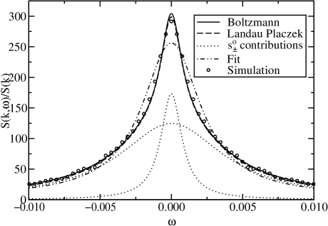
Figure 7: The central peak of the full spectrum at $\rho=6.5$, $P_{r}=0.05$, $\theta=0.05$, and $k_{x}=4\times 2\pi/512$. The Boltzmann spectrum and Landau Placzek formula overlap almost completely. The two isolated contributions of the central peaks in the later are indicated as well. The fit is made on the simulation results (points) with a single central peak only. Note that the two sound peaks fall outside the interval shown here.

In general the contributions forming the central peak cannot easily be separated. Even in the case they differ sufficiently in order to fit the central peak with two Lorentzians, one only obtains information on the values of $s^{\circ}_{\pm}$, which is not enough to determine the more interesting values of the thermal diffusivity and diffusion. An example of this is shown in Fig. 7 where we decomposed the central peak in the two Lorentzians using the theoretical expressions. For comparison we included the least square fit according to Eq.(59) to the full range of the spectrum, including the Brillouin peaks, where we only used a single Lorentz for the central peak.

For this reason it is important to consider the limits where decoupling occurs, since in those cases the the relevant transport values can be obtained from the spectra. Here we have however an interesting difference with respect to light scattering experiments Boon and Yip (1980). Whereas in that case the sensitivity of the dielectric fluctuations with respect to density is much larger than with respect to temperature, the amplitude factors will differ orders of magnitude. This results in the observation that the diffusion component will usually dominate the spectrum. For LGA this does not apply, and by using the decoupling limit $s^{\circ}_{\pm}\rightarrow\chi,{\cal D}$ on the first term off the Landau-Placzek formula (59), one immediately obtains that the central component of the spectrum is given by a single peak characterized by the thermal diffusivity

$$\frac{S^{\text{cen}}(\bm{k},\omega)}{S(\bm{k})}=\frac{\gamma-1}{\gamma}\frac{2\chi k^{2}}{\omega^{2}+(\chi k^{2})^{2}}.$$ (61)

One could in principle use this also in some of the intermediate cases seen in Fig. 3. The location of these points in terms of density and relative fractions, however, depends in a non-trivial way on the system parameters. Moreover, the identification with the thermal diffusivity and diffusion can only be made if one interpret $\chi$ and ${\cal D}$ as generalizations of these quantities.

IV.2 Red spectrum

The red dynamic structure factor can be evaluated by Hanon and Boon (1997); Blaak and Dubbeldam (2001a)

$$\frac{S^{\text{red}}(\bm{k},\omega)}{S(\bm{k})}=2\text{Re}\frac{\langle R|(e^{\imath\omega+\imath\bm{k}\cdot\bm{c}}-1-\Omega)^{-1}+\frac{1}{2}|R\rangle}{\langle R|R\rangle}.$$ (62)

It is possible to follow the same route for the red dynamic structure factor as for the full spectrum. However, since $\langle\rho|d\rangle=0$, but $\langle R|d\rangle\not=0$, it is more convenient to use a different set of basic invariants

$$|a_{n}\rangle=\{|c_{x}\rangle,|c_{y}\rangle,|p\rangle=|\frac{1}{2}c^{2}\rangle,|s_{r}\rangle=|p\rangle-\frac{\langle p|p\rangle}{\langle p|R\rangle}|R\rangle,|d_{r}\rangle\},$$ (63)

where $|d_{r}\rangle$ is constructed to be perpendicular to the other conserved quantities and defined by

$$|d_{r}\rangle=|p\rangle-\left(\frac{\langle p|R\rangle}{\langle R|R\rangle}|R\rangle-\frac{\langle p|R\rangle^{2}-\langle p|p\rangle\langle R|R\rangle}{\langle R|R\rangle\langle p|B\rangle}|B\rangle\right).$$ (64)

Note that by construction it is perpendicular to the red density, i.e. $\langle R|d\rangle=0$. Analogous to the case of the normal density we introduce some transport-like coefficients related to this basis

$$\chi_{\text{r}} =-\frac{\langle s_{r}|\frac{1}{\Omega}+\frac{1}{2}|s_{r}\rangle}{\langle s_{r}|s_{r}\rangle},$$ (65)

$${\cal D}_{\text{r}} =-\frac{\langle d_{r}|\frac{1}{\Omega}+\frac{1}{2}|d_{r}\rangle}{\langle d_{r}|d_{r}\rangle},$$ (66)

$$\gamma_{\text{r}} =1+\frac{\langle s_{r}|s_{r}\rangle}{\langle p|p\rangle}.$$ (67)

Obviously, the sound damping $\Gamma$, the modes $s^{\circ}_{\pm}$, and the speed of sound $c_{s}$ are all unchanged, since these are true transport values and independent of a chosen set of basis functions. Also in this case we can derive a Landau-Placzek formula, describing the red power-spectrum in the hydrodynamical domain

$$\frac{S^{\text{red}}(\bm{k},\omega)}{S(\bm{k})}=\frac{\gamma_{\text{r}}-1}{\gamma_{\text{r}}}\left[\left(1+\frac{\chi_{\text{r}}-{\cal D}_{\text{r}}}{s^{\circ}_{+}-s^{\circ}_{-}}\right)\frac{s^{\circ}_{+}k^{2}}{\omega^{2}+(s^{\circ}_{+}k^{2})^{2}}+\left(1-\frac{\chi_{\text{r}}-{\cal D}_{\text{r}}}{s^{\circ}_{+}-s^{\circ}_{-}}\right)\frac{s^{\circ}_{-}k^{2}}{\omega^{2}+(s^{\circ}_{-}k^{2})^{2}}\right]$$

$$+\frac{1}{\gamma_{\text{r}}}\left[\frac{\Gamma k^{2}}{(\omega+c_{s}k)^{2}+(\Gamma k^{2})^{2}}+\frac{\Gamma k^{2}}{(\omega-c_{s}k)^{2}+(\Gamma k^{2})^{2}}\right]$$

$$+\frac{1}{\gamma_{\text{r}}}\left[(\nu-\Gamma)+2(\gamma_{\text{r}}-1)\chi_{\text{r}}\right]\frac{k}{c_{s}}\left[\frac{\omega+c_{s}k}{(\omega+c_{s}k)^{2}+(\Gamma k^{2})^{2}}-\frac{\omega-c_{s}k}{(\omega-c_{s}k)^{2}+(\Gamma k^{2})^{2}}\right].$$ (68)

In principle the quantities $\chi_{\text{r}}$, ${\cal D}_{\text{r}}$, and $\gamma_{\text{r}}$ can be expressed in the normal transport values. However, these relations lead to more complex expressions and are for that reason omitted here. In Fig. 6 this formula is compared with the full Boltzmann red spectrum for a wave vector in the hydrodynamic regime, yielding a satisfactory approximation, and one in the kinetic regime with a large discrepancy.

IV.3 Diffusion spectrum

Finally we like to consider the spectra of the diffusive processes only. Due to the nature of LGA, however, it is not obvious how to define diffusion properly. On the one hand we have the requirement that a diffusive process is not propagating, on the other hand one expects the diffusion only to be related to the densities of both components in the mixture. As we will show in this section, it turns out that these two views are not completely compatible.

In the colored GBL model Blaak and Dubbeldam (2001a) and in the continuous case McLennan (1988) a diffusion spectrum can be obtained by considering fluctuations in the normalized difference of the red and blue density

$$\rho_{\text{diff}}=\frac{\rho_{\text{red}}}{P_{r}}-\frac{\rho_{\text{blue}}}{P_{b}}.$$ (69)

The proper translation in terms of invariants is given by

$$|\text{diff}\rangle=\frac{|R\rangle}{P_{r}}-\frac{|B\rangle}{P_{b}}.$$ (70)

However, a spectrum based on this vector, does not lead to purely diffusive peaks only, but also includes parts of the propagating modes. This can easily be checked since the vector is in general not orthogonal to the two soundmodes due to the absence of equipartition.

A simple solution is to subtract the propagating part by adding the appropriate term proportional to $|p\rangle$

$$|\text{diff}\rangle=\frac{|R\rangle}{P_{r}}-\frac{|B\rangle}{P_{b}}-\left(\frac{\langle p|R\rangle}{P_{r}}-\frac{\langle p|B\rangle}{P_{b}}\right)\frac{|p\rangle}{\langle p|p\rangle}.$$ (71)

In a binary athermal mixture Ernst and Dufty (1990), however, it was suggested to use

$$|\text{diff}\rangle=\frac{|R\rangle}{\langle R|R\rangle}-\frac{|B\rangle}{\langle B|B\rangle}.$$ (72)

Unfortunately this choice also leads to a propagating mode in the thermal case. One could again subtract the propagating part, but the result would be different from (71). The origin of this problem is that we have two different diffusive modes and any linear combination would lead to a diffusive spectrum. However, due to the lack of equipartition the different choices of fluctuations one wishes to consider do not coincide, not even after the propagating part is eliminated.

Naively one would expect a combination of the red and blue component only and in addition it should be perpendicular to the propagating modes. This leads to the following generalization of the athermal result (72), which in the case of an athermal model would coincide

$$|\text{diff}\rangle=\frac{|R\rangle}{\langle p|R\rangle}-\frac{|B\rangle}{\langle p|B\rangle}.$$ (73)

Obviously there is some freedom here in order to choose the generalization of the diffusion. The natural extension would be one that that satisfies the appropriate limits. However, in the low density limit and in the limit $P_{r}\rightarrow 1$, they all converge to the same value equal to the one found for the single component GBL model. The special case of an equal density for red and blue particles is not helpful either. This limit can be completely analyzed in a manner analogous to what is done for colored GBL model Blaak and Dubbeldam (2001a). For reasons of symmetry this will cause none of the definitions to have a propagating character and the resulting diffusions would coincide.

In Appendix B we derive the proper definition (100) for the transport values related to these quantities. Since none of them are proportional to a single eigenmode the usual formulation (33) is no longer valid. The results can be found in Fig. 8, where the diffusions obtained for the various diff’s are shown as function of the density. In general the five different diff’s described above all lead to different values for the corresponding transport value, although depending on the choice of system parameters this difference might be marginal. Also compare with Fig. 3 to see the difference with respect to ${\cal D}$.

Although the choice (73) is the most natural generalization, the diffusion is only properly identified in the limiting cases. In general some arbitrariness remains in a binary thermal lattice gas.

The corresponding diffusion spectrum is obtained by

$$\frac{S(\bm{k},\omega)}{S(\bm{k})}=2\text{Re}\frac{\langle\text{diff}|(e^{\imath\omega+\imath\bm{k}\cdot\bm{c}}-1-\Omega)^{-1}+\frac{1}{2}|\text{diff}\rangle}{\langle\text{diff}|\text{diff}\rangle}.$$ (74)

and shown in Fig. 9 for two diff’s: the $|\text{diff}\rangle$ defined in Eq. (72) based on an athermal model and the correct adjustment for the thermal model Eq. (73). For comparison we also included the curve for which the propagating part in Eq. (72) is subtracted as was described above. The first diffusion spectrum has a Brillouin-like pair of peaks which is a manifestation of the propagating part of $|\text{diff}\rangle$ according to (72), while the other two are different superpositions of two Lorentzians characterized by ${s_{\pm}}^{(0)}$.

Figure 8: A comparison of the different diff’s as a function of the density at $\theta=0.05$ and $P_{r}=0.75$. The curves labeled by a * are corrected by subtracting the propagating part as is described in the text. The diffusion according to Eq. (70) is not shown explicitly but overlaps on this scale with its corrected counterpart.

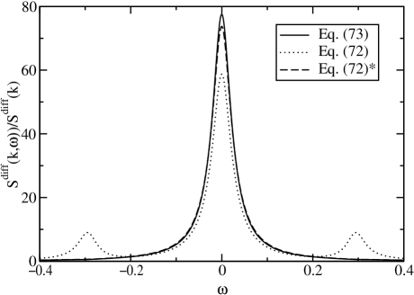
Figure 9: The Boltzmann diffusion spectrum based on Eqns. (72) and (73). The curve labeled by a * is corrected by subtracting the propagating part as is described in the text. The system parameters are $P_{r}=0.15$, $\rho=10.0$, and $\theta=0.05$. The wavevector $\bm{k}$ is given in reciprocal lattice units, the frequency $\omega$ in reciprocal time.

V Simulation results

We have verified our results with simulation results. Some notes on the implementation are in order. The model we consider is a true $38$-bits model, i.e. the collision operator can act on $2^{38}$ different states. In a previous article we reported the simulation results of a colored GBL model Blaak and Dubbeldam (2001a). The number of states in that model was $3^{19}$, since no red and blue particle could exist with the same velocity. The simulations could, however, be performed by realizing that the collisions could be separated in a normal GBL collision followed by a redistribution of the colors over the different particles present. These two separated processes can easily be performed by any computer.

In the present model this approach can not be used. One could of course make use of the symmetries present in the model. The hexagonal lattice leads to six rotations and two reflections. In addition we can make use of the interchange of red and blue particles, and the interchange of particles and holes. At best this would lead to a reduction with a factor of 48 on the total number of different states, but in practice this factor is less because a large fraction of the states is invariant with respect to some of these symmetries. This is however still too large in order to be applied in any but the largest supercomputers available at present. An alternative, but rather inefficient scheme, would be to store only part of the collision table and generate other collisions on the fly.

Binary mixtures, however, do allow for a more convenient solution, which is less efficient than storing the complete collision table, but still has a relative good performance (about a factor 2-5 slower than the colored GBL model). Rather than storing a collision table based on the states, we make one based on the different classes. In the GBL model there are $29926$ different classes ${\cal C}=(M,\bm{P},E)$, characterized by the total mass, momentum, and energy. Since the the binary mixture is the combination of two GBL models there are $29926^{2}$ different combinations $({\cal C}_{R},{\cal C}_{B})$ of a red and blue class which form a total of $4478568$ classes $\Gamma=(M_{r},M_{b},\bm{P},E)$. If we combine this with the 48 symmetry operations we get a working algorithm that already can be used on a computer with 256 MB of memory.

An arbitrary input state is now analyzed in order to determine to which class $\Gamma$ it belongs. From its characterization one can easily find which transformation is needed in order put it in a form with $M_{R}\leq M_{B}$, $M_{R}+M_{B}\leq 19$, and $0\leq P_{y}\leq P_{x}/\sqrt{3}$. The last inequality confines the total momentum to an angle of $\pi/6$. For each $\Gamma$ in this limited set of classes only, all the classes ${\cal C}_{R}$, that with the appropriate class ${\cal C}_{B}$ can give rise to it, have been stored, including the number of states in each $({\cal C}_{R},{\cal C}_{B})$ combination. From this we generate with the proper weight an “outgoing” class combination to which the inverse transformation is applied. Finally we only need to determine a random state in ${\cal C}_{R}$ and ${\cal C}_{B}$, which is just a GBL-like process.

Simulation results along with the Boltzmann approximation and the Landau-Placzek formula are shown in Fig. 6 for both the normal and red spectrum. In the Figs. 6a and 6b the spectra at low $\bm{k}$ value completely overlap and the Landau-Placzek formula describes the power spectrum very well. If we increase the wavevector $\bm{k}$, and/or lower the density, the hydrodynamical regime is left and deviations start to appear. In that generalized regime, the transport properties are $\bm{k}$-dependent. Figs. 6c and 6d show a spectrum even further away from the hydrodynamic regime, in the kinetic regime. Several kinetic modes invade the spectrum, and a parameterization into Lorentzians has lost all physical meaning. The full spectrum based on the Boltzmann approximation, however, still leads to a very good description, supporting the molecular chaos assumption.

VI Discussion

We have constructed a thermal binary lattice gas mixture. The model is characterized by cross-effects between energy transport and diffusion. The Landau-Placzek formula derived in the the low wavevector, low frequency domain gives an excellent description. For larger wavevectors it will fail, but the spectra can still accurately be described by the Boltzmann approximation.

The Landau-Placzek formula for a regular binary thermal mixture is quite similar in structure as the one for the continuous case. The main feature is a central peak formed by two Lorentzians due to the coupled entropy-concentration fluctuations. In the limits of low density, single specie, their dual interpretations, and equal red and blue density it is possible for the central peak of the spectrum to be decomposed into two Lorentzians with linewidths given by $\chi\bm{k}^{2}$ and ${\cal D}\bm{k}^{2}$, otherwise the linewidths depend on both these values.

In the low density limit the true modes $s^{\circ}_{\pm}$ converge to $\chi$ and ${\cal D}$. Moreover, they can be identified with the thermal diffusivity and mass-diffusion coefficient of the GBL model and coincide with the low density limit of the continuous binary mixture. In contrast with continuous theory, however, it is the thermal diffusivity that dominates the central part of the spectrum, rather than the diffusion. The interpretation of $\chi$ as the thermal diffusivity can be extended to the general situation. For ${\cal D}$ this not true, since the related spectrum will contain Brillouin peaks, which is a not a purely diffusive property. Although it is possible to correct for this, there remains some ambiguity in the choice for the generalized diffusion coefficient.

The analysis and results presented here are in general true for binary thermal lattice gasses and not restricted to this particular model only. It also reduces automatically to the proper formulation for an athermal model, in which case some of the ambiguities are removed.

Appendix A

To calculate terms of the type ${\cal N}_{\mu}$ given in Eq. (56) we express the left eigenvectors in terms of right eigenvectors, and expand ${\cal N}_{\mu}$ to linear order in $k$

$${\cal N}_{\mu}= \frac{\langle\rho|\psi_{\mu}^{(0)}\rangle^{2}}{\langle\psi_{\mu}^{(0)}|\psi_{\mu}^{(0)}\rangle}\left(1+2\imath k\left[\frac{\langle\rho|\psi_{\mu}^{(1)}\rangle}{\langle\rho|\psi_{\mu}^{(0)}\rangle}-\frac{\langle\psi_{\mu}^{(0)}|\psi_{\mu}^{(1)}\rangle}{\langle\psi_{\mu}^{(0)}|\psi_{\mu}^{(0)}\rangle}\right]+\right.$$ (75)

$$\left.\imath k\left[\frac{\langle\rho|c_{\ell}\psi_{\mu}^{(0)}\rangle}{\langle\rho\psi_{\mu}^{(0)}\rangle}-\frac{\langle\psi_{\mu}^{(0)}|c_{\ell}\psi_{\mu}^{(0)}\rangle}{\langle\psi_{\mu}^{(0)}|\psi_{\mu}^{(0)}\rangle}\right]+{\cal O}(k^{2})\right).$$

As can be seen from the second term on the righthand side, partial knowledge of the $|\psi_{\mu}^{(1)}\rangle$ is required. From the formal solution (30) of the first order equation and the orthogonality relation (29) it follows that we only need to evaluate the coefficients $B_{\mu\nu}$. From the normalization (19) we already know that $B_{\mu\mu}=0$. In addition we like to mention that from symmetry considerations one can conclude that the mode related to the viscosity will not contribute. Hence the values of $B_{\mu\perp}$ and $B_{\perp\mu}$ need not be determined.

In order to facilitate the calculations we first list some simple relations

$$\langle\psi_{\sigma}^{(0)}|\psi_{\sigma}^{(0)}\rangle=2\langle p|p\rangle,$$ (76)

$$\langle\rho|\psi_{\sigma}^{(0)}\rangle=\langle\rho|p\rangle,$$ (77)

$$\langle\rho|s_{\pm}\rangle=\frac{(1-\gamma)}{\sqrt{\langle s|s\rangle}}\langle\rho|p\rangle,$$ (78)

$$\langle s_{\pm}|s_{\pm}\rangle=2\sqrt{1+\xi^{2}}\left(\sqrt{1+\xi^{2}}\mp\xi\right).$$ (79)

Most coefficients can be evaluated from the relation (34). In the case of the soundmodes this leads to

$$B_{\sigma,-\sigma}=-\frac{\langle j_{-\sigma}|\frac{1}{\Omega}+\frac{1}{2}|j_{\sigma}\rangle}{(z_{\sigma}^{(1)}-z_{-\sigma}^{(1)})\langle\psi_{-\sigma}^{(0)}|\psi_{-\sigma}^{(0)}\rangle}$$ (80)

and with the use of $|j_{\pm}\rangle=|j_{s}\rangle\pm c_{s}|\tau_{xx}\rangle$ this can be rewritten in terms of the basic transport coefficients

$$B_{\sigma,-\sigma}=\sigma\frac{\nu-(\gamma-1)\chi}{4c_{s}}=\frac{\sigma(\nu-\Gamma)}{2c_{s}}.$$ (81)

The next coefficient we need to evaluate is

$$B_{s_{\pm},\sigma}=-\frac{\langle j_{\sigma}|\frac{1}{\Omega}+\frac{1}{2}|j_{s_{\pm}}\rangle}{(z_{s_{\pm}}^{(1)}-z_{\sigma}^{(1)})\langle\psi_{\sigma}^{(0)}|\psi_{\sigma}^{(0)}\rangle},$$ (82)

and here we can use the same relation to rewrite the current of the soundmodes. For the other current the relation (37) can be used. Realizing that the terms containing $|\tau_{xx}\rangle$ will vanish, the remaining terms can be manipulated to yield

$$B_{s_{\pm},\sigma}=(\gamma-1)\frac{\sigma s^{\circ}_{\pm}}{2c_{s}\sqrt{\langle s|s\rangle}}.$$ (83)

From Eq. (34) we can now also see that

$$B_{\sigma,s_{\pm}}=-\frac{\langle\psi_{\sigma}^{(0)}|\psi_{\sigma}^{(0)}\rangle}{\langle s_{\pm}|s_{\pm}\rangle}B_{s_{\pm},\sigma}=-\left(1\pm\frac{\xi}{\sqrt{1+\xi^{2}}}\right)\frac{\sigma s^{\circ}_{\pm}\sqrt{\langle s|s\rangle}}{2c_{s}}.$$ (84)

The last two coefficients which we will need are $B_{s_{\pm},s_{\mp}}$. However, since $z_{s_{\pm}}^{(1)}=0$ they can not be obtained from (34). In order for them to be determined we need to make use of the third order equation of the eigenvalue problem (13)

$$\Omega|\psi_{\mu}^{(3)}\rangle = (c_{\ell}+z_{\mu}^{(1)})|\psi_{\mu}^{(2)}\rangle+\left[z_{\mu}^{(2)}+\frac{1}{2}(c_{\ell}+z_{\mu}^{(1)})^{2}\right]|\psi_{\mu}^{(1)}\rangle+$$ (85)

$$\left[z_{\mu}^{(3)}+z_{\mu}^{(2)}(c_{\ell}+z_{\mu}^{(1)})+\frac{1}{6}(c_{\ell}+z_{\mu}^{(1)})^{3}\right]|\psi_{\mu}^{(0)}\rangle.$$

As we only want to determine the values of $B_{s_{\pm},s_{\mp}}$, we do not attempt to solve the complete third order equation but restrict ourselves to the two equations from which they can be obtained. Note that we have $z_{s_{\pm}}^{(1)}=0$ and hence $|j_{s_{\pm}}\rangle=|c_{\ell}s_{\pm}\rangle$.

Substituting these results in the third order equation, replacing $\mu$ by $s_{\pm}$, and multiplying on the left with the appropriated term $\langle s_{\mp}|$ we find

$$0=\langle s_{\mp}|c_{\ell}|\psi_{s_{\pm}}^{(2)}\rangle+\langle s_{\mp}|s^{\circ}_{\pm}+\frac{1}{2}c_{\ell}^{2}|\psi_{s_{\pm}}^{(1)}\rangle+\langle s_{\mp}|z_{s_{\pm}}^{(3)}+s^{\circ}_{\pm}c_{\ell}+\frac{1}{6}c_{\ell}^{3}|s_{\pm}\rangle.$$ (86)

The last term will disappear due to the odd power of $c_{\ell}$ and because $\langle s_{\mp}|s_{\pm}\rangle=0$. In order to proceed we not only need the solution of the first order equation (30) but also solution of the second order equation. Fortunately the later does not have to be computed completely but the formal solution will suffice

$$|\psi_{\mu}^{(2)}\rangle=\frac{1}{\Omega}(c_{\ell}+z_{\mu}^{(1)})|\psi_{\mu}^{(1)}\rangle+\frac{1}{\Omega}\left(z_{\mu}^{(2)}+\frac{1}{2}(c_{\ell}+z_{\mu}^{(1)})^{2}\right)|\psi_{\mu}^{(0)}\rangle+$$

$$\sum_{\nu}C_{\mu\nu}|\psi_{\nu}^{(0)}\rangle,$$ (87)

where the $C_{\mu\nu}$ are some unknown coefficients. Substitution of both solutions in Eq. (86) gives

$$0=\langle s_{\mp}|c_{\ell}\frac{1}{\Omega}c_{\ell}|\psi_{s_{\pm}}^{(1)}\rangle+\langle s_{\mp}|c_{\ell}\frac{1}{\Omega}\left(s^{\circ}_{\pm}+\frac{1}{2}c_{\ell}^{2}\right)|s_{\pm}\rangle+\sum_{\nu}C_{s_{\pm}\nu}\langle j_{s_{\mp}}|\psi_{\nu}^{(0)}\rangle+$$

$$\langle s_{\mp}|\left(s^{\circ}_{\pm}+\frac{1}{2}c_{\ell}^{2}\right)\frac{1}{\Omega}|c_{\ell}s_{\pm}\rangle+\sum_{\nu}B_{s_{\pm}\nu}\langle s_{\mp}|\left(s^{\circ}_{\pm}+\frac{1}{2}c_{\ell}^{2}\right)|\psi_{\nu}^{(0)}\rangle.$$ (88)

The second and fourth term on the right are zero because of the odd power in $c_{\ell}$, the third term is zero because of the orthogonality relations (28). Another substitution of the first order solution leads to

$$0= \langle s_{\mp}|c_{\ell}\frac{1}{\Omega}c_{\ell}\frac{1}{\Omega}c_{\ell}|s_{\pm}\rangle+\sum_{\nu}B_{s_{\pm}\nu}\langle s_{\mp}|c_{\ell}\frac{1}{\Omega}c_{\ell}|\psi_{\nu}^{(0)}\rangle+$$ (89)

$$\sum_{\nu}B_{s_{\pm}\nu}\langle s_{\mp}|\left(s^{\circ}_{\pm}+\frac{1}{2}c_{\ell}^{2}\right)|\psi_{\nu}^{(0)}\rangle.$$

The first term is again zero because of the odd power in $c_{\ell}$. Writing out the sum, using the orthogonality relations, and realizing that the shear mode dependent term cancels due to symmetries this leads to

$$B_{s_{\pm},s_{\mp}}s^{\circ}_{\pm}\langle s_{\mp}|s_{\mp}\rangle+B_{s_{\pm},s_{\mp}}\langle j_{s_{\mp}}|\frac{1}{\Omega}+\frac{1}{2}|j_{s_{\mp}}\rangle+$$

$$B_{s_{\pm},+}\langle j_{s_{\mp}}|\frac{1}{\Omega}+\frac{1}{2}|c_{\ell}\psi_{+}^{(0)}\rangle+B_{s_{\pm},-}\langle j_{s_{\mp}}|\frac{1}{\Omega}+\frac{1}{2}|c_{\ell}\psi_{-}^{(0)}\rangle=0.$$ (90)

From symmetry considerations it follows that the terms with $|\psi_{\pm}^{(0)}\rangle$ only contribute via $|p\rangle$ and by using the definition of the transport values on the second term we obtain

$$B_{s_{\pm},s_{\mp}}(s^{\circ}_{\pm}-s^{\circ}_{\mp})\langle s_{\mp}|s_{\mp}\rangle+(B_{s_{\pm},+}+B_{s_{\pm},-})\langle j_{s_{\mp}}|\frac{1}{\Omega}+\frac{1}{2}|c_{\ell}p\rangle=0.$$ (91)

Using the expressions for $B_{s_{\pm},\sigma}$ and the fact that $s^{\circ}_{+}$ and $s^{\circ}_{-}$ are different, it follows that $B_{s_{\pm},s_{\mp}}=0$.

The evaluation of the ${\cal N}$ now becomes straightforward. The last term at the righthand site of Eq. (75) will vanish because of symmetry reasons. From the second term it can be observed that even if we would not have chosen $B_{\mu\mu}=0$ as a normalization, this coefficient would not contribute to the spectrum. For the viscosity we immediately obtain ${\cal N}_{\perp}=0$. In the case of $\mu=\sigma$ this results in

$${\cal N}_{\sigma} = \frac{\langle\rho|p\rangle^{2}}{2\langle p|p\rangle}\left(1+2\imath k\left[B_{\sigma,-\sigma}+B_{\sigma,s_{+}}\frac{\langle\rho|s_{+}\rangle}{\langle\rho|\psi_{\sigma}^{(0)}\rangle}+B_{\sigma,s_{-}}\frac{\langle\rho|s_{-}\rangle}{\langle\rho|\psi_{\sigma}^{(0)}\rangle}\right]\right),$$ (92)

$$= \frac{\langle\rho|\rho\rangle}{2\gamma}\left(1+\frac{\imath\sigma k}{c_{s}}\left[\Gamma+(\gamma-1)\chi\right]\right),$$

where in the second line we have eliminated the viscosity. The $|s_{\pm}\rangle$ lead to

$${\cal N}_{s_{\pm}} = \frac{(\gamma-1)^{2}\langle\rho|p\rangle^{2}}{2\langle s_{\pm}|s_{\pm}\rangle}\left(1+2\imath k\left[B_{s_{\pm},+}\frac{\langle\rho|\psi_{+}^{(0)}\rangle}{\langle\rho|s_{\pm}^{(0)}\rangle}+B_{s_{\pm},-}\frac{\langle\rho|\psi_{-}^{(0)}\rangle}{\langle\rho|s_{\pm}\rangle}\right]\right),$$ (93)

$$= \frac{(\gamma-1)\langle\rho|\rho\rangle}{2\gamma}\left(1\pm\frac{\xi}{\sqrt{1+\xi^{2}}}\right),$$

where the imaginary part cancels completely.

Appendix B

In general one defines a transport coefficient via the decay of small fluctuations with respect to the equilibrium distribution. If we take $\delta f(\bm{k})$ to be such a fluctuation, we obtain for a single timestep

$$e^{z(\bm{k})}=\frac{\langle\delta f|e^{-\imath\bm{k}\cdot\bm{c}}(\bm{1}+\Omega)|\delta f\rangle}{\langle\delta f|\delta f\rangle},$$ (94)

where the second order term in $k$ of $z(\bm{k})$ will be the transport coefficient.

Naturally these fluctuations can always be written in terms of the eigenfunctions of the linearized Boltzmann operator

$$|\delta f(\bm{k})\rangle=\sum_{\mu}\frac{\langle\psi_{\mu}|\delta f\rangle}{\langle\psi_{\mu}|\psi_{\mu}\rangle}|\psi_{\mu}(\bm{k})\rangle,$$ (95)

where the coefficients on the right-hand site are independent of $\bm{k}$ and therefore can be obtained from the $k=0$ limit $\langle\psi_{\mu}|\delta f\rangle/\langle\psi_{\mu}|\psi_{\mu}\rangle=\langle\psi_{\mu}^{(0)}|\delta f^{(0)}\rangle/\langle\psi_{\mu}^{(0)}|\psi_{\mu}^{(0)}\rangle$. Combining this formal expansion with Eq. (94) and using the results of the eigenvalue problem (13) we obtain

$$e^{z(\bm{k})}=\frac{1}{\langle\delta f|\delta f\rangle}\sum_{\mu}\frac{\langle\psi_{\mu}|\delta f\rangle}{\langle\psi_{\mu}|\psi_{\mu}\rangle}\langle\delta f|e^{z_{\mu}}|\psi_{\mu}\rangle.$$ (96)

If we restrict ourselves to fluctuations proportional to the hydrodynamic modes, and thus assume the exponential fast decay of the kinetic modes, the eigenvalues $e^{z_{\mu}}$ can be expanded in terms of $\bm{k}$. This results in

$$e^{z(\bm{k})}=1+\sum_{\mu}\frac{\langle\psi_{\mu}|\delta f\rangle\langle\delta f|\psi_{\mu}\rangle}{\langle\psi_{\mu}|\psi_{\mu}\rangle\langle\delta f|\delta f\rangle}\left(\imath kz_{\mu}^{(1)}-k^{2}\left[z_{\mu}^{(2)}+\frac{1}{2}(z_{\mu}^{(1)})^{2}\right]\right)+{\cal O}(k^{3}).$$ (97)

Note that the prefactors also depend on $\bm{k}$, but can be rewritten as

$$\frac{\langle\psi_{\mu}|\delta f\rangle\langle\delta f|\psi_{\mu}\rangle}{\langle\psi_{\mu}|\psi_{\mu}\rangle\langle\delta f|\delta f\rangle}=\left(\frac{\langle\psi_{\mu}^{(0)}|\delta f^{(0)}\rangle}{\langle\psi_{\mu}^{(0)}|\psi_{\mu}^{(0)}\rangle}\right)^{2}\frac{\langle\psi_{\mu}|\psi_{\mu}\rangle}{\langle\delta f|\delta f\rangle}=$$

$$\frac{\langle\psi_{\mu}^{(0)}|\delta f^{(0)}\rangle\langle\delta f^{(0)}|\psi_{\mu}^{(0)}\rangle}{\langle\psi_{\mu}^{(0)}|\psi_{\mu}^{(0)}\rangle\langle\delta f^{(0)}|\delta f^{(0)}\rangle}+{\cal O}(k^{2}).$$ (98)

This allows us to calculate the lowest order terms of $z(\bm{k})$ via

$$z^{(1)}=\sum_{\mu}\frac{\langle\psi_{\mu}^{(0)}|\delta f^{(0)}\rangle\langle\delta f^{(0)}|\psi_{\mu}^{(0)}\rangle}{\langle\psi_{\mu}^{(0)}|\psi_{\mu}^{(0)}\rangle\langle\delta f^{(0)}|\delta f^{(0)}\rangle}z_{\mu}^{(1)}$$ (99)

$$z^{(2)}+\frac{1}{2}\left(z^{(1)}\right)^{2}=\sum_{\mu}\frac{\langle\psi_{\mu}^{(0)}|\delta f^{(0)}\rangle\langle\delta f^{(0)}|\psi_{\mu}^{(0)}\rangle}{\langle\psi_{\mu}^{(0)}|\psi_{\mu}^{(0)}\rangle\langle\delta f^{(0)}|\delta f^{(0)}\rangle}\left(z_{\mu}^{(2)}+\frac{1}{2}(z_{\mu}^{(1)})^{2}\right)$$ (100)

It can easily be checked that in the case of a single eigenmode for the fluctuation $\delta f$ these equations reduce to the normal results, in particular Eq. (33). In general, however, such a formulation in terms of currents is not valid. The fact that it nevertheless is consistent for Eqns. (41) and (42) is a consequence of the orthogonality relation (39) between the currents of the two diffusive eigenmodes.

In the case of the different diffusions calculated in Sec. IV.3 we need to make use of these equations, because the fluctuations under consideration are not eigenmodes. From symmetry arguments it follows that in all those cases $z^{(1)}=0$, and strictly speaking none of these fluctuations will therefore be propagating. In the case of Eqns. (70) and (72), however, the soundmodes will contribute to the transport value (100) and spectra based on these fluctuations will contain Brillouin peaks.

We finally like to mention that these results are only valid in the limit $k\rightarrow 0$ and for small times, because if one considers the decay for larger time intervals one would obtain

$$e^{z(\bm{k})t}=\frac{\langle\delta f|\left[e^{-\imath\bm{k}\cdot\bm{c}}(\bm{1}+\Omega)\right]^{t}|\delta f\rangle}{\langle\delta f|\delta f\rangle}=\sum_{\mu}\left(\frac{\langle\psi_{\mu}^{(0)}|\delta f^{(0)}\rangle}{\langle\psi_{\mu}^{(0)}|\psi_{\mu}^{(0)}\rangle}\right)^{2}\frac{\langle\psi_{\mu}|\psi_{\mu}\rangle}{\langle\delta f|\delta f\rangle}e^{z_{\mu}t}.$$ (101)

This results in a different behavior for short and long times in the case one considers fluctuations that are not proportional to a single eigenmode (See also Ref. Mountain and Deutch (1969)).

References

- Frisch et al. (1986) U. Frisch, B. Hasslacher, and Y. Pomeau, Lattice-Gas Automata for the Navier-Stokes Equation, Phys. Rev. Lett. 56, 1505–1508 (1986).
- Rivet and Boon (2001) J. P. Rivet and J. P. Boon, Lattice Gas Hydrodynamics, Cambridge Nonlinear Science Nr. 11 (Cambridge University Press, Cambridge, 2001).
- Chen et al. (1991) S. Chen, K. Diemer, G. D. Doolen, K. Eggert, C. Fu, S. Gutman, and J. Travis, Lattice gas automata for flow through porous media, Physica D 47, 72–84 (1991).
- Gunstensen and Rothman (1991) A. K. Gunstensen and D. H. Rothman, A Galilean-invariant immiscible lattice gas, Physica D 47, 53–63 (1991).
- Chopard et al. (1994) B. Chopard, P. Luthi, and M. Droz, Reaction-diffusion cellular automata model for the formation of Leisegang patterns, Phys. Rev. Lett. 72, 1384–1387 (1994).
- Malevanets and Kapral (1998) A. Malevanets and R. Kapral, Continuous-velocity lattice-gas model for fluid flow, Europhys. Lett. 44, 552–558 (1998).
- Baran et al. (1997) O. Baran, C. C. Wan, and R. Harris, A new thermal lattice gas, Physica A 239, 322–328 (1997).
- Rothman (1994) D. H. Rothman, Lattice-gas models of phase seperation: interfaces, phase transitions and multiphas flow, Rev. Mod. Phys. 66, 1417–1479 (1994).
- Brito et al. (1991) R. Brito, M. H. Ernst, and T. R. Kirkpatrick, Staggered Diffusivities in Lattice Gas Cellular Automata, J. Stat. Phys. 62, 283–295 (1991).
- Das and Ernst (1992) S. P. Das and M. H. Ernst, Thermal transport properties in a square lattice gas, Physica A 187, 191–209 (1992).
- Ernst and Das (1992) M. H. Ernst and S. P. Das, Thermal Cellular Automata Fluids, J. Stat. Phys. 66, 465–483 (1992).
- Ernst and Dufty (1990) M. H. Ernst and J. W. Dufty, Hydronamics abd Time Correlation Functions for Cellular Automata, J. Stat. Phys. 58, 57–86 (1990).
- Hanon and Boon (1997) D. Hanon and J. P. Boon, Diffusion and correlations in lattice-gas automata, Phys. Rev. E 56, 6331–6339 (1997).
- Blaak and Dubbeldam (2001a) R. Blaak and D. Dubbeldam, Boltzmann approximation of transport properties in thermal lattice gases, Phys. Rev. E 63, 021109 (2001a).
- Mountain and Deutch (1969) R. D. Mountain and J. M. Deutch, Light Scattering from Binary Solutions, J. Chem. Phys. 50, 1103–1108 (1969).
- Boon and Yip (1980) J. P. Boon and S. Yip, Molecular Hydrodynamics (McGraw-Hill Inc., New-York, 1980).
- Blaak and Dubbeldam (2001b) R. Blaak and D. Dubbeldam, Coupling of thermal and mass diffusion in regular binary thermal lattice-gases, Phys. Rev. E 64, 062102 (2001b).
- Grosfils et al. (1992) P. Grosfils, J.-P. Boon, and P. Lallemand, Spontaneous Fluctuation Correlations in Thermal Latice-Gas Automata, Phys. Rev. Lett. 68, 1077–1080 (1992).
- Grosfils et al. (1993) P. Grosfils, J.-P. Boon, R. Brito, and M. H. Ernst, Statistical hydrodynamics of lattice-gas automata, Phys. Rev. E 48, 2655–2668 (1993).
- Résibois and de Leener (1977) P. Résibois and M. de Leener, Classical Kinetic Theory of Fluids (Wiley, New-York, 1977).
- McLennan (1988) J. A. McLennan, Introduction to Non-Equillibrium Statistical Mechanics (Prentice Hall, Englewood Cliffs, New Jersey, 1988).