Non-Abelian phases, charge pumping, and quantum computation with Josephson junctions

Abstract

Non-Abelian geometric phases can be generated and detected in certain superconducting nanocircuits. Here we consider an example where the holonomies are related to the adiabatic charge dynamics of the Josephson network. We demonstrate that such a device can be applied both for adiabatic charge pumping and as an implementation of a quantum computer.

If a quantum system is prepared in a superposition of two states, a physical observable associated with this system can exhibit oscillatory behavior depending on the relative phase of the two states. Interference can be induced during the dynamical evolution of the system, in this case we refer to the accumulated phase as the dynamical phase. Interference can also be of geometrical nature if the parameters (coupling constants, external fields,$\dots$) of the Hamiltonian are varied cyclically [1]. After Berry’s original work, considerable attention has been devoted to the interpretation, generalization, and detection of geometric phases [2]. An important generalization is when the adiabatic cyclic evolution involves a degenerate eigenspace of the Hamiltonian. In this case it has been shown by Wilczek and Zee [3] that the evolution over a closed path does not result in a phase change but it leads to a superposition of the degenerate eigenstates and the geometric phase acquires a non-Abelian structure. Originally investigated in Nuclear Quadrupole Resonance [4], more recently it was shown that non-Abelian phases occur in the manipulation of trapped ions [5, 6].

Apart from its fundamental importance, geometric interference has interesting applications in the field of quantum information processing [7, 8]. Implementations of quantum computers so far include optical systems and liquid-state NMR [9] as well as solid-state devices based on superconductors [10] and on semiconductors [11]. Recently it has been shown that quantum computation can also be implemented by geometric means (geometric quantum computation) using Abelian [12] as well as non-Abelian [13, 6] phases.

Non-Abelian phases can also appear in the quantum dynamics of superconducting nanocircuits [14], this is what we will show in this work. There are various interesting aspects associated with this analysis. In addition to their possible detection, which is intriguing by itself, the existence of non-Abelian phases in superconducting nanocircuits leads to a new scheme for adiabatic charge pumping and allows to implement solid state holonomic quantum computation. Some parts of our proposal are on purpose speculative. The adiabatic manipulation of degenerate subspaces and the degeneracy condition itself is non-trivial to achieve for an artificially fabricated device. We believe, however, due to the rapid development in the control of artificial two-level systems in solid-state devices [15], the realization of geometric interference in mesoscopic systems has become plausible. Furthermore the applications of non-Abelian phases in pumping and computation are interesting new directions to pursue.

In our discussion of non-Abelian phases in Josephson junction circuits we follow the spirit of the schemes described in Refs.[5, 6]. The starting point is the network shown in Fig.1a). It consists of three superconducting islands labeled by $j=L,M,R$ (Left, Middle, Right) each of which is connected to a fourth (Upper) island labeled with $U$. Gate voltages are applied to the three bottom islands via gate capacitances. The device operates in the charging regime, that is the Josephson energies $J_{j}$ ($j=L,M,R$) of the junctions are much smaller than the charging energy $E_{C}$ of the setup. Each coupling is designed as a Josephson interferometer (a loop interrupted by two junctions and pierced by a magnetic field) as shown in Fig.1a. Thus the effective Josephson energies $J_{j}$ can be tuned by changing the flux in the corresponding loop. Electrostatic energies can be varied by changing the gate voltages $V_{g}$.

Let us first analyze the electrostatic problem (i.e. $J_{j}\equiv 0$). For the sake of simplicity we assume that all capacitances are equal to $C$ and we consider identical gate charges $\displaystyle{q_{g}=C_{g}V_{g}/(2e)}$ for the three bottom islands. The charge states are indicated as $\mid n_{U},n_{L},n_{M},n_{R}\rangle$ where $n$ labels the number of Cooper pairs in the corresponding island [16]. For gate charges $\displaystyle{q_{g}\simeq 1/2}$ and $\displaystyle{1<2q_{U}+3q_{g}<2}$ (where $\displaystyle{q_{U}=C_{U}V_{U}/(2e)}$, see Fig.1a), only four charge states are important as long as $T\ll E_{C}=(2e)^{2}/(4C)$. Three of these charge states, $\mid 0,1,0,0\rangle,\mid 0,0,1,0\rangle,\mid 0,0,0,1\rangle$ are degenerate. Their charge configuration corresponds to one excess Cooper pair in one of the islands $j=L,C,R$, and none in the island $U$. The fourth state $\mid 1,0,0,0\rangle$ has one excess pair on the island $U$ and none on the other islands. All other charge states are much higher in energy.

The Josephson couplings $J_{j}$ allow for tunneling between the upper island and each of the bottom islands. The quantum-mechanical Hamiltonian of this simple four-state system reads (in complete analogy with Refs.[5, 6])

$$H=\delta E_{C}|1,0,0,0\rangle\langle 1,0,0,0|+\frac{1}{2}\bigl{[}J_{L}(\bar{\Phi}_{L})|1,0,0,0\rangle\langle 0,1,0,0|\ +\,$$ (1)

$$~{}~{}~{}~{}+J_{M}(\bar{\Phi}_{M})|1,0,0,0\rangle\langle 0,0,1,0|+J_{R}(\bar{\Phi}_{R})|1,0,0,0\rangle\langle 0,0,0,1|+{\rm H.c.\/}\bigr{]}\,$$ (2)

where $\displaystyle{\delta E_{C}=\frac{4}{5}E_{C}\left[(q_{g}-q_{U})-\frac{1}{2}\right]}$ is the energy difference between the three degenerate states and the fourth one, and $\bar{\Phi}_{j}=\Phi_{j}/\Phi_{0}$ are the external magnetic fluxes in units of the flux quantum $\Phi_{0}=hc/2e$ [17]. In all the manipulations described below the gate voltages will be kept fixed. The three fluxes $\displaystyle{\{\bar{\Phi}_{L},\bar{\Phi}_{M},\bar{\Phi}_{R}\}}$ are the parameters which will be varied cyclically. In general all the SQUID loops could be asymmetric, although it is not necessary for the purpose of our discussion.

The Hamiltonian defined in Eq.(2) can easily be diagonalized. The lowest and highest eigenstate are non-degenerate. The peculiar feature, exploited in [5, 6] is that the other two states (with zero energy) are degenerate for arbitrary values of the couplings $J_{j}$. The subspace is spanned by the eigenstates (not normalized)

$$|D_{1}\rangle=-J_{M}|0,1,0,0\rangle\ +J_{L}|0,0,1,0\rangle\ ,$$ (3)

$$|D_{2}\rangle=-J_{R}\left(J_{L}^{*}|0,1,0,0\rangle+J_{M}^{*}|0,0,1,0\rangle\right)+(|J_{L}|^{2}+|J_{M}|^{2})|0,0,0,1\rangle.$$ (4)

By manipulation of the external magnetic fluxes it is possible to generate non-Abelian phases. We will show that by means of such phases adiabatic charge pumping and holonomic quantum computation can be realized with superconducting nanocircuits.

Charge pumping - For this purpose it is sufficient to have only symmetric SQUID loops. In contrast to the well-known turnstiles for single electrons or Cooper pairs [18, 19, 20] (in which the gate potentials are modulated periodically), here charge is transported through the chain (from the L-island to the R-island) by means of modulating the Josephson couplings while keeping the gate voltages unchanged. The pumping cycle goes as follows. The system is initially prepared in the $|0,1,0,0\rangle$ state (i.e.the state $|D_{1}\rangle$ with $J_{L},J_{M}=0$ ) where the Cooper pair is in the left island. This can be achieved by turning off all Josephson couplings and coupling the L-island to a lead which provides the extra Cooper pair. Once the charge is on the island, one should change adiabatically the magnetic fluxes along a closed loop $\gamma$. At the end of the loop the initially prepared stated $|D_{1}\rangle$ will be mapped into the following rotated state: $|D_{1}\rangle\longrightarrow U_{\gamma}|D_{1}\rangle,$ where the unitary matrix $U_{\gamma}$ may be expressed as [3]:

$$U_{\gamma}={\bf P}\exp\oint_{\gamma}\sum_{j=L,M,R}A_{j}d\bar{\Phi}_{j}\,;~{}~{}~{}(A_{j})_{\alpha,\beta}=\langle D_{\alpha}|\frac{\partial}{\partial\bar{\Phi}_{j}}|D_{\beta}\rangle,~{}~{}~{}\alpha,\beta=1,2.\;$$ (5)

Path ordering P is required as, in general, the matrices $A_{j}$ do not commute along the path. If the path $\gamma$ is chosen in the $(\bar{\Phi}_{L},\bar{\Phi}_{R})$- plane (at fixed $\bar{\Phi}_{M}=0$), as shown in Fig.1b it can be shown that, after one adiabatic cycle, the final state of the system is $|0,0,0,1\rangle$, i.e. one Cooper pair has been transported through the chain of the three islands [21].

The mechanism described here relies entirely on the geometric phase accumulated during the cycle and can be generalized to describe pumping of a single Cooper pair through $N$ superconducting islands. The connection between pumping and geometric phases has been discussed by Pekola et al. [20]. The crucial difference is that here only the Josephson couplings have to be varied. During the cycle, exactly one Cooper pair is transported, in this sense there are no errors due to the spread of the wave function discussed in  [20]. There are drawbacks though, mostly related to the fact that the degenerate states are not the ground state and relaxation processes may become important.

Quantum computation, one qubit - The pumping process illustrated so far is nothing but one of the key elements to construct a quantum computing scheme using non-Abelian phases. Proceeding along the lines of Ref.[6], we point out the necessary ingredients and the differences which arise in the case of the Josephson junction setup. The nanocircuit presented in Fig.1a constitutes the qubit. The logical states to encode information in this implementation are

$$|0\rangle_{\ell} = |0,1,0,0\rangle$$ (6)

$$|1\rangle_{\ell} = |0,0,0,1\rangle\ \ .$$ (7)

The other two charge states ($|1,0,0,0\rangle$ and $|0,0,1,0\rangle$) serve as auxiliary states. To show that the implementation is possible, it is sufficient to provide explicit representations for the gates $U_{1}=e^{i\Sigma_{1}|1\rangle_{\ell\ell}\langle 1|}$ and $U_{2}=e^{i\Sigma_{2}\sigma_{y}}$, describing rotations of the qubit state about the $z$ axis and the $y$ axis, respectively. In this case only one asymmetric SQUID (as shown in Fig.1) is required to implement the one-qubit operations.

The gate $U_{1}$ is a phase shift for the state $|1\rangle_{\ell}$ while the state $|0\rangle_{\ell}$ remains decoupled, i.e., $J_{L}\equiv 0$ during the operation. In the initial state we have $J_{R}=0$, so the eigenstates $\{|D_{1}\rangle,|D_{2}\rangle\}$ correspond to the logical states $\{|0\rangle_{\ell},|1\rangle_{\ell}\}$. The control parameters $\bar{\Phi}_{M},\bar{\Phi}_{R}$ evolve adiabatically along the closed loop $C_{1}$ in the $(\bar{\Phi}_{M},\bar{\Phi}_{R})$-plane from $\displaystyle{\bar{\Phi}_{R}=1/2}$ to $\displaystyle{\bar{\Phi}_{R}=1/2}$ (see Fig.2a). By using the formula for holonomies Eq.(5) one can show that this cyclic evolution produces the gate $U_{1}$ with the phase $\Sigma_{1}$ :

$$\Sigma_{1}=\sigma_{1}\oint_{{\cal S}(C_{1})}d\bar{\Phi}_{\rm M}d\bar{\Phi}_{R}\frac{\sin\left(2\pi\bar{\Phi}_{R}\right)}{\left(|J_{R}(\bar{\Phi}_{R})|^{2}+|J_{M}(\bar{\Phi}_{M})|^{2}\right)^{2}}\,$$ (8)

where ${\cal S}(C_{1})$ denotes the surface enclosed by the loop $C_{1}$ in ${\cal M}$. and $\sigma_{1}=4\pi^{2}J_{R}(0)^{2}(|J_{Ml}|^{2}-|J_{Mr}|^{2})$.
Similarly we can consider a closed loop $C_{2}$ (see Fig.2b) in the $(\bar{\Phi}_{L},\bar{\Phi}_{R})$-plane at fixed $\bar{\Phi}_{\rm M}=0$, and let the control parameters $\bar{\Phi}_{L}$ and $\bar{\Phi}_{R}$ undergo a cyclic adiabatic evolution with starting and ending point $\displaystyle{\bar{\Phi}_{L}=\bar{\Phi}_{R}=1/2}$. This operation yields the gate $U_{2}$ with phase $\Sigma_{2}$

$$\Sigma_{2}=\sigma_{2}\oint_{{\cal S}(C_{2})}d\bar{\Phi}_{R}d\bar{\Phi}_{L}\frac{\sin\left(\pi\bar{\Phi}_{L}\right)\sin\left(\pi\bar{\Phi}_{R}\right)}{\left(J_{M}(0)^{2}+|J_{R}(\bar{\Phi}_{R})|^{2}+|J_{L}(\bar{\Phi}_{L})|^{2}\right)^{3/2}}$$ (9)

where ${\cal S}(C_{2})$ denotes the surface enclosed by the loop $C_{2}$ in ${\cal M}$, and $\sigma_{2}=4\pi^{2}|J_{R}(0)|^{2}(|J_{Ml}|^{2}+|J_{Mr}|^{2})$ where we have assumed $J_{L}(0)=J_{R}(0)$. Obviously the pumping cycle discussed above is a special case of the gate $U_{2}$ with $\Sigma_{2}=\pi/2$.

Quantum computation, two qubits - It turns out that it is possible to implement a conditional phase shift $U_{3}=e^{i\Sigma_{3}|11\rangle_{\ell\ell}\langle 11|}$ by coupling two qubits via Josephson junctions. These junctions should be realized as symmetric SQUID loops such that the coupling can be switched off. The capacitive coupling due to these SQUID loops can be neglected if the capacitances of the junctions are sufficiently small [22].

By setting $\delta E_{C}=0$ (this was not necessary in the one-qubit case) and by coupling the qubits as shown in Fig.3a) we obtain the Hamiltonian

$$H_{\rm 2qubit}=\frac{1}{2}\left[J^{(2)}_{M}|{UU}\rangle\langle{UM}|+J_{X}|11\rangle_{\ell}\langle{UU}|+{\rm H.c.}\right]\$$ (10)

where we introduced the notation $|U\rangle=|1,0,0,0\rangle$ and $|M\rangle=|0,0,1,0\rangle$ for the auxiliary states which are coupled by the interaction between the qubits. The matrix element $J_{X}=J_{X}(\bar{\Phi}_{\em UR},\bar{\Phi}_{\em RU})$ is given by $J_{X}=-(1/2)J_{UR}(\bar{\Phi}_{\em UR})\,J_{\em RU}(\bar{\Phi}_{\em UR})\,\mu$ where $\displaystyle{\mu=\left[1/\delta E_{C}^{+-}+1/\delta E_{C}^{-+}\right]}$. Here $\delta E_{C}^{+-}$ and $\delta E_{C}^{-+}$ denote the charging energy difference between the initial and the intermediate state (see below). The coupling is of second order in the Josephson energies since the inter-qubit coupling junctions change the total number of pairs on each one-bit setup. Thus the coupling occurs via intermediate charge states which lie outside the Hilbert space of the two-qubit system. These are states, e.g. $|0,0,0,0\rangle\otimes|1,0,0,1\rangle$, without excess Cooper pair on the first qubit and two excess pairs on the second qubit. We have abbreviated the charging energy difference between the corresponding state and the initial qubit state by $\delta E_{C}^{-+}$, and we have denoted the external magnetic fluxes in the coupling SQUID loops by $\Phi_{\em UR}$ and $\Phi_{\em RU}$.

While $J_{X}(\bar{\Phi}_{\em UR},\bar{\Phi}_{\em RU})$ is the only off-diagonal coupling of second order, there are also second-order corrections of the diagonal elements, i.e. of the energies of the two-qubit states. These corrections would lift the degeneracy and thus would hamper the geometric operation which is based on the degeneracy of all states. It is therefore crucial that it is possible to compensate these corrections and to guarantee the degeneracy. It is easy to see that by adjusting the gate voltages the energy shifts can be canceled. Note that during the geometric operation the values of the Josephson couplings are changing and therefore also the energy shifts are not constant. Consequently their compensation by means of the gate voltages has to follow the evolution of the parameters.
Let us now show explicitly how the gate $U_{3}$ can be achieved. To this aim, we consider a closed loop $C_{3}$ in the $(\bar{\Phi}^{(2)}_{\em M},\bar{\Phi}_{\em UR})$-plane at fixed $\bar{\Phi}_{\em RU}=0$. (See Fig.3b). If the control parameters $\bar{\Phi}_{\em UR}$ and $\bar{\Phi}_{\em M}^{(2)}$ undergo a cyclic adiabatic evolution with starting and ending point $\bar{\Phi}_{\em UR}=1/2$, $\bar{\Phi}_{\em M}^{(2)}=0$, the geometric phase obtained with this loop is

$$\Sigma_{3}=\sigma_{3}\oint_{{\cal S}(C_{3})}d\bar{\Phi}_{M}^{(2)}d\bar{\Phi}_{UR}\frac{\mu^{2}\sin\left(2\pi\bar{\Phi}_{UR}\right)}{\left(|J_{M}^{(2)}(\bar{\Phi}_{M}^{(2)})|^{2}+\mu^{2}\,J_{RU}(0)^{2}|J_{UR}(\bar{\Phi}_{UR})|\right)^{2}}$$

with $\sigma_{3}=4\pi^{2}J_{RU}(0)^{4}(|J_{{M}l|}^{2}-|J_{{M}r}|^{2})$ and $J_{UR}(0)=J_{RU}(0)$.

As we have mentioned in the introduction, some caution is required before regarding this scheme ready for implementation. In practice it will be difficult to achieve perfect degeneracy of all states. Thus the question is imposed to which extend incomplete degeneracy of the qubit states is permissible. Clearly, the adiabatic condition requires the inverse operation time $\tau_{\rm op}$ to be smaller than the minimum energy difference to the neighboring states: $\tau_{\rm op}^{-1}\ll\min{\delta E_{C},J_{j},J_{X}}$. On the other hand, if the degeneracy is not complete and the deviation is of the order $\epsilon$ one can show by modifying the derivation of Eq. (4) in Ref.[13] that for $\epsilon\ll\tau_{\rm op}^{-1}$ the holonomies can be realized to a sufficient accuracy. This inequality expresses the requirement that the operation time be still small enough in order to not resolve small level spacings of the order $\epsilon$.

There is another important constraint on $\tau_{\rm op}$. As the degenerate states in Eq. (4) are different from the ground state of the system, $\tau_{\rm op}$ must not be too large in order to prevent inelastic relaxation. The main origin for such relaxation processes is the coupling to a low-impedance electromagnetic environment. We can estimate the relaxation rate by $\Gamma_{\rm in}\sim E(R_{\rm env}/R_{K})$ where $R_{K}=h/e^{2}$ is the quantum resistance and $E$ is on the order of the Josephson energies $E\sim J_{j},J_{X}$. Thus it is not difficult to satisfy the condition $\tau_{\rm op}<\Gamma_{\rm in}^{-1}$ experimentally. In fact, it has been found recently that inelastic relaxation times in charge qubits can be made quite large and exceed by far the typical dephasing times due to background charge fluctuations [23, 24, 25].

Both charge pumping and the implementation of quantum computing are related to coherent manipulations of charge states. Therefore as a readout one can use the scheme developed [10] to measure charge qubits. No additional difficulty is forecasted at this level.

Stimulating discussions with G. Falci, G.M. Palma, E. Paladino, M. Rasetti and P. Zanardi are gratefully acknowledged. We wish to thank M.-S. Choi for informing us of his results. This work has been supported by the EU (IST-FET SQUBIT) and by INFM-PRA-SSQI.

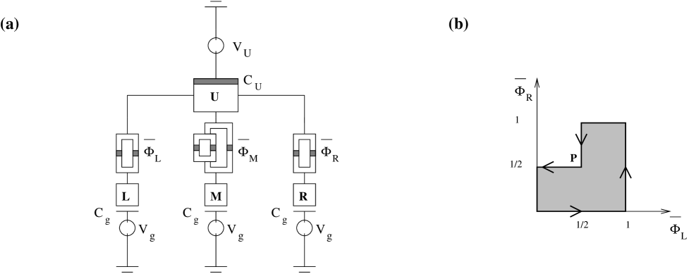
FIG. 1.: a)Elementary Josephson network for the investigation of non-Abelian geometric phases. Note that an asymmetric SQUID loop cannot be switched off completely [17]. Since $J_{\rm M}=0$ may be desirable for quantum computation the SQUID is designed such that this condition can be satisfied; b)Pumping cycle for $3$ islands. Starting from $P=(1/2,1/2)$ and adiabatically following the drawn path, the gate $\displaystyle{U=e^{i\frac{\pi}{2}\sigma_{y}}}$ can be achieved.

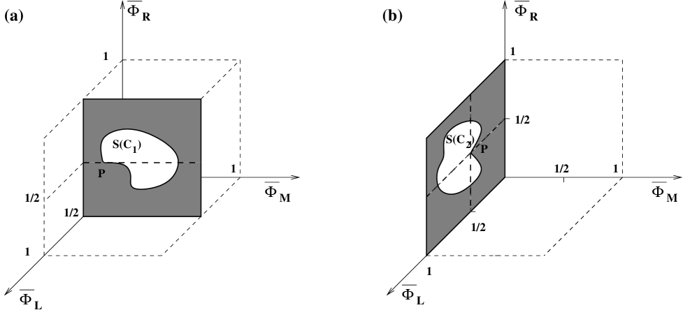
FIG. 2.: Geometric realizations of gates $U_{1}=e^{i\Sigma_{1}|1\rangle_{\ell\ell}\langle 1|}$ (a) and $U_{2}=e^{i\Sigma_{2}\sigma_{y}}$ (b). The structure (non-zero elements) of the unitary matrices $U_{1}$ and $U_{2}$ is determined by the choice of the plane containing the loop and by the starting/ending point of the closed path. Different values of phase $\Sigma_{1}$ $(\Sigma_{2})$ can be obtained by varying the area enclosed by loops $C_{1}$ $(C_{2})$.

FIG. 3.: Inter-qubit coupling for the implementation of the gate $U_{3}$ and its geometric realization.

REFERENCES

- [1] M.V. Berry, Proc. Roy. Soc. A 392, 45 (1984).
- [2] Geometric phases in physics, A. Shapere and F. Wilczek, Eds. World Scientific, (Singapore, 1989).
- [3] F. Wilczek and A. Zee, Phys. Rev. Lett. 52, 2111 (1984).
- [4] R. Tycko, Phys. Rev. Lett. 58, 2281 (1987).
- [5] R.G. Unanyan, B.W. Shore, and K. Bergmann, Phys. Rev. A 59, 2910 (1999).
- [6] L.-M. Duan, J.I. Cirac, and P. Zoller, Science 292, 1695 (2001).
- [7] M. Nielsen and I. Chuang, Quantum Computation and Quantum Communication, (Cambridge University Press, Cambridge, 2000).
- [8] A. Ekert and R. Jozsa, Rev. Mod. Phys. 68, 733-753 (1996).
- [9] D. DiVincenzo, Fortschr. Phys. 48, 771 (2000)
- [10] Yu. Makhlin, G. Schön, and A. Shnirman Rev. Mod. Phys. 73, 357 (2000).
- [11] G. Burkard, H.-A. Engel, and D. Loss, Fortschr. Phys. 48, 965 (2000).
- [12] J. Jones, V. Vedral, A.K. Ekert, C. Castagnoli, Nature, 403, 869 (2000); G. Falci, R. Fazio, G.M. Palma, J. Siewert, and V. Vedral, Nature 407, 355 (2000); Wang Xiang-Bin and Matsumoto Keiji, Phys. Rev. Lett. 97, 097901 (2001); A. Blais, A.-M.S. Tremblay, quant-ph/0105006; F.K. Wilhelm and J.E. Mooij, unpublished (2001).
- [13] P. Zanardi and M. Rasetti, Phys. Lett. A 264, 94 (1999); J. Pachos, P. Zanardi and M. Rasetti, Phys. Rev. A 61, R10305 (2000); J. Pachos, quant-ph/00031150.
- [14] While completing this work we became aware of a similar proposal by M.-S. Choi, quant-ph/0111019.
- [15] T.H. Oosterkamp et al. Nature 395, 873 (1998); Y. Nakamura, Yu. Pashkin, and J.S. Tsai, Nature 398, 786 (1999); D. Vion, et al., Science 296, 886 (2002)
- [16] We ignore quasiparticles since they are suppressed at low temperature.
- [17] In the case of an asymmetric SQUID loop is a complex number whose modulus and phase are and where , denote the Josephson energies of the left and right junction of each SQUID loop in Fig. 1. Tinkham M., Introduction to Superconductivity, 2nd edition, McGraw-Hill, (New York, 1996)
- [18] H. Pothier et al., Physica B 169, 573 (1991).
- [19] L.J. Geerligs et al., Z. Phys. B 85, 349 (1991).
- [20] J.P. Pekola et al., Phys. Rev. B 60, R9931 (1999).
- [21] We mention finally that one can imagine to realize this pumping mechanism also in a setup of semiconducting islands; B.L. Altshuler and L.I. Glazman, Science 283, 1864 (1999).
- [22] J. Siewert and R. Fazio, Phys. Rev. Lett. 87, 257905 (2001).
- [23] Y. Nakamura, Yu.A. Pashkin, T. Yamamoto, J.S. Tsai, Phys. Rev. Lett. 88, 047901 (2002).
- [24] E. Paladino, L. Faoro, G. Falci, and R. Fazio, Phys. Rev. Lett. 88, 228304 (2002).
- [25] The effect of an environment on the observability of the geometric phases requires further analysis, see R.S. Whitney and Y. Gefen, cond-mat/0208141.