Antiferromagnetism in the Exact Ground State of the Half Filled Hubbard Model on the Complete-Bipartite Graph

Abstract

As a prototype model of antiferromagnetism, we propose a repulsive Hubbard Hamiltonian defined on a graph $\Lambda={\cal A}\cup{\cal B}$ with ${\cal A}\cap{\cal B}=\emptyset$ and bonds connecting any element of ${\cal A}$ with all the elements of ${\cal B}$. Since all the hopping matrix elements associated with each bond are equal, the model is invariant under an arbitrary permutation of the ${\cal A}$-sites and/or of the ${\cal B}$-sites. This is the Hubbard model defined on the so called $(N_{A},N_{B})$-complete-bipartite graph, $N_{A}$ ($N_{B}$) being the number of elements in ${\cal A}$ (${\cal B}$). In this paper we analytically find the exact ground state for $N_{A}=N_{B}=N$ at half filling for any $N$; the repulsion has a maximum at a critical $N$-dependent value of the on-site Hubbard $U$. The wave function and the energy of the unique, singlet ground state assume a particularly elegant form for $N\rightarrow\infty$. We also calculate the spin-spin correlation function and show that the ground state exhibits an antiferromagnetic order for any non-zero $U$ even in the thermodynamic limit. We are aware of no previous explicit analytic example of an antiferromagnetic ground state in a Hubbard-like model of itinerant electrons. The kinetic term induces non-trivial correlations among the particles and an antiparallel spin configuration in the two sublattices comes to be energetically favoured at zero Temperature. On the other hand, if the thermodynamic limit is taken and then zero Temperature is approached, a paramagnetic behavior results. The thermodynamic limit does not commute with the zero-Temperature limit, and this fact can be made explicit by the analytic solutions.

I Introduction

The Hubbard Hamiltonian is one of the most popular models to describe strongly correlated electron systems. In spite of its simple definition, it can be exactly solved only in few cases. An example is the milestone solution of the Hubbard ring[1] by means of the Bethe-Ansatz[2] extended to fermions[3][4]. Other exact solutions were worked out for the one-dimensional Hubbard ring in the presence of an external magnetic field[5], for the one-dimensional Hubbard chain with open boundary conditions[6] and thereafter for the $SU(N)$ one-dimensional Hubbard ring[7]. However, when the space dimensionality becomes bigger than 1, few exact results are available and usually they concern the ground state properties. Among them, we mention the Lieb theorem on the ground state spin degeneracy[8] that will be explicitly used in this work. Exact ground state wave functions are even more infrequent. To the best of our knowledge the only non-trivial results are the ferromagnetic ground-state solutions devised by Nagaoka[9] (infinite repulsion and one hole over the half filled system), by Mielke and Tasaki[10][11] (for which the kinetic energy spectrum is macroscopically degenerate or at least very flat) and by Wang[12] (infinite-range hopping).

In the Hubbard Hamiltonian with infinite-range hopping a particle in any site can hop to any other site of the system; the associated graph is said to be complete. This model was numerically studied by Patterson on small clusters[13] in 1972 and solved in the thermodynamic limit by van Dongen and Vollhardt[14] only at the end of the eighties. Much more effort was needed to find the exact ground state(s) in the finite-size system. Verges et al. managed to accomplish this task for arbitrary numbers of particles and sites in the limit of infinite on-site repulsion $U$[15] by exploiting a scheme proposed by Brandt and Giesekus [16]. Two years later Wang constructed explicitly the ground states of the system for arbitrary $U$ and number of particles above half filling[12]. In the case of one particle added over the half-filled system the ferromagnetic ground-state solution follows as a special (and the easiest) case of general results by Mielke and Tasaki[17].

In this paper we find the exact ground state wave function of the half-filled Hubbard model on the Complete-Bipartite Graph (CBG) for arbitrary but finite $U$. The CBG $\Lambda={\cal A}\cup{\cal B}$ has bonds connecting any element of ${\cal A}$ with all the elements of ${\cal B}$ and can be considered as the natural further step (with respect to the complete graph previously described) towards the standard Hubbard Hamiltonian (defined on the hypercubic lattice and hopping between nearest-neighbours sites). Even if the CBG is still somewhat unrealistic, we feel that exact solutions should always be welcome, expecially because they lend themselves to be generalized. Furthermore, our solution is an example of antiferromagnetic ground state in a model of itinerant electrons, in contrast with the ferromagnetic solutions mentioned above; it may provide useful hints about antiferromagnetism outside of the strong coupling regime (where the Hubbard model can be mapped onto the Heisenberg model).

The paper has been organized as follows. In Section II we define the model and discuss the physics of the non-interacting ($U=0$) Hamiltonian together with few relevant examples of finite-size realizations. In Section III we study the thermodynamic limit of a class of Hubbard-like models, which includes the Hubbard Hamiltonian on the complete graph and on the complete bipartite graph, having a non-extensive number of isolated one-particle energy levels plus a single level whose degeneracy is proportional to the size of the system. Following the reasoning of van Dongen and Vollhardt[14], we show that the kinetic term is totally decoupled from the interaction term and that the system behaves as a paramagnet: the spin-spin correlation length is zero. These results are a consequence of the trivial behaviour of such models any time the thermodynamic limit is taken first. On the contrary, much more difficult is to find exact properties in finite-size systems and different answers may be obtained if the thermodynamic limit is taken only at the end of the calculations (as we shall show in Section VI). In Section IV we introduce the essential tools to face the problem. Let $N=N_{A}=N_{B}$ be the number of sites of each sublattice ${\cal A}$ and ${\cal B}$. First, we find a ($2N-2$)-body determinantal eigenstate $|\Phi_{AF}\rangle$ of the Hamiltonian with vanishing double occupation; then, we demonstrate that it is a key tool to build the ground state. We show that mapping the ${\cal A}$-sites onto the ${\cal B}$-sites and viceversa, $|\Phi_{AF}\rangle$ retains its form except for a spin-flip; we shall call this property the antiferromagnetic property. Several analogies with the properties of the half-filled standard $N\times N$ Hubbard model are pointed out at this stage. Here we also deal with the spin projection of $|\Phi_{AF}\rangle$ onto the singlet and the triplet subspace and useful identities between the two spin-projected states are obtained. Then, in Section V we propose an Ansatz for the ground state wave function at half filling containing the singlet and triplet projections of $|\Phi_{AF}\rangle$. We set up the Schrödinger equation and by exploiting the antiferromagnetic property we close the equations and get 3 exact eigenstates. The ground-state uniqueness proved by Lieb[8] is used to show that the lowest-energy state of our Ansatz actually corresponds to the ground state of the system. Remarkably, the ground state energy is negative for any value of the repulsion $U$; qualitatively, we may say that the particles manage to avoid the double occupation very effectively. In Section VI we study the ground state energy $E_{0}$ as a function of $U$ and of the volume of the system and we discuss the implications of exchanging the thermodynamic limit with the limit of zero temperture. We find that $E_{0}$ is a monotonically increasing function of $U$ and $N$ due to the existence of non-trivial correlations even for large $N$. The nature of these correlations is investigated by computing the expectation value of the repulsion. We show that for any finite $N$ there is a critical value of $U$ yielding maximum repulsion. From the exact spin-spin correlation function we find that the ground state average of the staggered magnetization operator squared is exstensive. Hence, the ground state is antiferromagnetically ordered; we underline that this holds not only at strong coupling, but for any value of $U$. Finally, a summary of the main results and conclusions are drawn in Section VII.

II Definition of the Model

Let $\Lambda={\cal A}\cup{\cal B}$ with ${\cal A}\cap{\cal B}=\emptyset$ be a collection of sites and

$$|{\cal A}|=N_{A},\;\;|{\cal B}|=N_{B}\;\Rightarrow|\Lambda|=N_{A}+N_{B}\;.$$ (1)

Here and in the following we shall denote by $|{\cal S}|$ the number of elements in the set ${\cal S}$. We consider the Hubbard Hamiltonian

$$H_{{\mathrm{H}ubbard}}=H_{0}+W,\;\;\;H_{0}=\sum_{x,y\in\Lambda}\sum_{\sigma}t_{x,y}c^{{\dagger}}_{x\sigma}c_{y\sigma},\;\;\;W=U\sum_{x\in\Lambda}\hat{n}_{x\uparrow}\hat{n}_{x\downarrow}$$ (2)

where $c_{x\sigma}$ ($c^{{\dagger}}_{x\sigma}$) is the annihilation (creation) operator of a particle at site $x$ with spin $\sigma=\uparrow,\downarrow$ and $\hat{n}_{x\sigma}=c^{{\dagger}}_{x\sigma}c_{x\sigma}$ is the corresponding particle number operator. The hopping matrix $T$ with elements $T_{x,y}=t_{x,y}=t_{y,x}$ is a real-symmetric matrix while $U$ is a positive constant. If

$$t_{x,y}=\left\{\begin{array}[]{ll}\tilde{t}&{\mathrm{f}or}\;x\in{\cal A}\;(x\in{\cal B})\;{\mathrm{a}nd}\;y\in{\cal B}\;(y\in{\cal A})\\ 0&{\mathrm{o}therwise}\end{array}\right.$$ (3)

the graph $\Lambda$ is said to be complete bipartite and we call the Hamiltonian in Eq.(2) the CBG-Hubbard Hamiltonian. The model is invariant under an arbitrary permutation of the ${\cal A}$-sites and/or of the ${\cal B}$-sites. Therefore, the symmetry group includes $S_{N_{A}}\otimes S_{N_{B}}$, $S_{N}$ being the set of permutations of $N$ objects. As usual, the full group is much bigger: the presence of spin and pseudospin symmetries[8][18] leads to an $SO(4)$ internal symmetry Group[19][20] and in the case $N_{A}=N_{B}$ there is a $Z_{2}$ symmetry because of the ${\cal A}\leftrightarrow{\cal B}$ exchange.

In Fig.(1) we have drawn a few examples of finite-size systems. For $N=1$ and $N=2$ the model is equivalent to a one dimensional ring of length $L=2,\;4$ respectively. For $N=3$ we have what can be understood as a prototype, (1,1) nanotube model, the one of smallest length $L=1$, with periodic boundary conditions. For general $N$, one can conceive a gedanken device, like the one illustrated pictorially for $N=6$ in Fig.(1.$d$). (The whole device should actually have the topology of a torus, and the two horizontal faces should coincide, but this is not shown in the Figure for the sake of clarity.) The $N$ vertical lines represent a realization of the ${\cal A}$ sublattice while the ${\cal B}$ sublattice is mimicked by the central object. The radial tracks in the Figure represent conducting paths linking each ${\cal A}$ site to each ${\cal B}$ site according to the topology of our model. The ${\cal A}$ sites are represented by one-dimensional electron-in-a-box systems of length $L$. Each ${\cal A}$ site has the one-body energy spectrum $\varepsilon_{{\mathrm{f}ree}}\sim n^{2}/mL^{2}$ where $n$ is an integer and $m$ is the electron mass. We assume that $L$ is so small that the excited states are at high energy and can be disregarded in the low-energy sector; this requires $mL^{2}\ll 1/U$. Here, of course, $U$ denotes the Coulomb self-energy of a box with two electrons. The ${\cal B}$ sites are hosted by $N$ quantum dots, that can be represented by $\delta$-function-like attractive potential wells of depth $V$; if $|V|$ is large and the radius of the dots is $\ll L$, these are practically independent of each other. The one-body energy of each ${\cal B}$ site is $\varepsilon_{{\mathrm{b}ound}}\sim-mV^{2}$; the unbound states can be neglected if $mV^{2}\gg U$. We are assuming for simplicity that the $U$ of the ${\cal B}$ sites is the same as for the ${\cal A}$ ones. Turning on a constant potential $V_{0}$ on the central object, one can arrange that the Hubbard Hamiltonian on the CBG $H_{{\mathrm{H}ubbard}}$ gives a good description of the system, with filling $\leq 2$ per site.

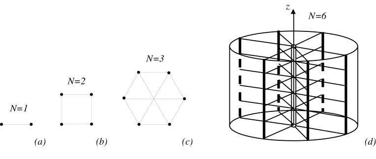
FIG. 1.: Physical representation of the CBG for $N=1$ ($a$) and $N=2$ ($b$) which is equivalent to a one dimensional ring of length $L=2,\;4$ respectively. For $N=3$ ($c$) we have the (1,1) nanotube of smallest length and periodic boundary conditions. For $N=6$ ($d$) we present the gedanken device described in the text.

It is convenient to label each site with an integer in such a way that $x=1,\ldots,N_{A}$ corresponds to sites in ${\cal A}$ and $x=N_{A}+1,\ldots,N_{A}+N_{B}$ corresponds to sites in ${\cal B}$. In the special case $N_{A}=N_{B}=N$ the hopping matrix can be written as

$$T=\tilde{t}\left(\begin{array}[]{ll}Z&J\\ J&Z\end{array}\right)$$ (4)

where $Z$ is the $N\times N$ null matrix and $J$ is the $N\times N$ matrix whose generic element $J_{x,y}=1$. The one-body spectrum has three different eigenvalues

$$\varepsilon_{g} = -N\tilde{t}\equiv-t\;\;$$ (5)

$$\varepsilon_{0} = 0\;\;$$ (6)

$$\varepsilon_{\bar{g}} = N\tilde{t}\equiv t$$ (7)

with degeneracy $d_{g}=1$, $d_{0}=2N-2$ and $d_{\bar{g}}=1$ respectively. We use the convention $t>0$ so that $\varepsilon_{g}$ is the lowest level and we shall call ${\cal S}_{hf}$ the set of zero-energy one-body eigenstates.

The orthogonal matrix $O$ that diagonalizes $T$ can be written in the form

$$O=\left(\begin{array}[]{ll}\begin{array}[]{c}\frac{1}{\sqrt{2N}}\;\frac{1}{\sqrt{2N}}\ldots\\ R\\ Z_{r}\\ \frac{1}{\sqrt{2N}}\;\frac{1}{\sqrt{2N}}\ldots\end{array}&\begin{array}[]{c}\frac{-1}{\sqrt{2N}}\;\frac{-1}{\sqrt{2N}}\ldots\\ Z_{r}\\ R\\ \frac{1}{\sqrt{2N}}\;\frac{1}{\sqrt{2N}}\ldots\end{array}\end{array}\right)$$ (8)

where $Z_{r}$ is the $(N-1)\times N$ rectangular null matrix, while $R$ is an $(N-1)\times N$ rectangular matrix whose rows are orthonormal vectors which are orthogonal to the $N-$dimensional vector $(1,1,\ldots,1,1)$. The zero-energy one-body orbitals can be visualized by a simple argument. Consider any pair $x,\;y$, with $x\neq y,$ of sites belonging to the same sublattice, say ${\cal A}$, and a wavefunction $\psi_{x,y}$ taking the values 1 and -1 on the pair and 0 elsewhere in ${\cal A}$ and in ${\cal B}$. It is evident that $\psi_{x,y}$ belongs to ${\cal S}_{hf}$. Operating on $\psi_{x,y}$ by the permutations of $S_{N}$ we can generate a (non-orthogonal) basis of $N-1$ eigenfunctions[21] vanishing in ${\cal B}$; further, by means of the $Z_{2}$ symmetry, we obtain the remaining orbitals of ${\cal S}_{hf}$, which vanish on ${\cal A}$. This exercise shows that the group considered above justifies the ($2N-2$)-fold degeneracy of the one-body spectrum.

Having obtained the one-body basis, one can form a suitable $R$ matrix by orthogonalization. Let us define the transformed operators:

$$g\equiv\sum_{x=1}^{2N}O_{1,x}c_{x}=\frac{1}{\sqrt{2N}}\sum_{x=1}^{N}(c_{x}-c_{x+N})$$ (9)

$$a_{i}\equiv\sum_{x=1}^{2N}O_{i+1,x}c_{x}=\sum_{x=1}^{N}R_{i,x}c_{x},\;\;i=1,\ldots,N-1$$ (10)

$$b_{i}\equiv\sum_{x=1}^{2N}O_{i+N,x}c_{x}=\sum_{x=1}^{N}R_{i,x}c_{x+N},\;\;i=1,\ldots,N-1$$ (11)

$$\bar{g}\equiv\sum_{x=1}^{2N}O_{2N,x}c_{x}=\frac{1}{\sqrt{2N}}\sum_{x=1}^{N}(c_{x}+c_{x+N}).$$ (12)

The inverse transformation reads

$$c_{x}=\frac{1}{\sqrt{2N}}(g+\bar{g})+\sum_{i}R_{i,x}a_{i},\;\;x\in{\cal A}$$ (13)

$$c_{x}=\frac{1}{\sqrt{2N}}(-g+\bar{g})+\sum_{i}R_{i,x-N}b_{i},\;\;x\in{\cal B}$$ (14)

and the kinetic term $H_{0}$ becomes

$$H_{0}=-t\sum_{\sigma}(g^{{\dagger}}_{\sigma}g_{\sigma}-\bar{g}^{{\dagger}}_{\sigma}\bar{g}_{\sigma})\;.$$ (15)

Hence, if we do not rescale the hopping constant, the average kinetic energy remains an extensive quantity proportional to $N\tilde{t}$: the kinetic energy of the two particles in the lowest level coincides with the kinetic energy of the whole system. On the other hand, if $\tilde{t}\sim 1/N$ the two energy gaps $\varepsilon_{0}-\varepsilon_{g}$ and $\varepsilon_{\bar{g}}-\varepsilon_{0}$ remain constant as $N$ increases. As we shall show in the next Section, the model can be exactly solved in the thermodynamic limit whatever is the dependence of $\varepsilon_{g}$ and $\varepsilon_{\bar{g}}$ on $|\Lambda|$.

III Thermodynamic Limit

The Hubbard Hamiltonian on the CBG (as on the complete graph) belongs to a class of Hubbard-like models that can be exactly solved in the thermodynamic limit. Here we generalize the results by van Dongen and Vollhardt[14] to the case of a non-extensive number of non-vanishing one-body eigenenergies and in the presence of a local external magnetic field coupled to the spin of the particles. Even if the reasoning is similar to that of Ref.[14], a detailed presentation of the main results is needed to clarify more subtle points and make our work self-contained. Furthermore, some of the results are absent in the original paper and we believe that their derivation will facilitate the reader in the comprehension of what follows.

Let us consider the Hamiltonian

$$H=H_{{\mathrm{H}ubbard}}-\mu\sum_{x\in\Lambda}\sum_{\sigma}\hat{n}_{x\sigma}-\sum_{x\in\Lambda}h_{x}(\hat{n}_{x\uparrow}-\hat{n}_{x\downarrow})\equiv H_{{\mathrm{H}ubbard}}+H_{\mu}+H_{h}$$ (16)

where $H_{{\mathrm{H}ubbard}}=H_{0}+W$ is defined in Eq.(2), $\mu$ is the chemical potential and $H_{h}$ represents the coupling with an external magnetic field. Let us assume that only a finite number f of eigenvalues of the hopping matrix $T$ are non-vanishing, $\varepsilon_{i}\neq 0$ for $i=1,\ldots,$f, while the remaining $|\Lambda|-$f are identically zero. Denoting with $\phi_{i}$ and $\phi^{{\dagger}}_{i}$ the annihilation and creation operators that diagonalize $H_{0}$ we have

$$H_{0}=\sum_{i=1}^{{\mathrm{f}}}\sum_{\sigma}\varepsilon_{i}\phi^{{\dagger}}_{i\sigma}\phi_{i\sigma}$$ (17)

and the CBG corresponds to the case f=2, see Eq.(15). The Gran-Partition Function ${\cal Z}_{\beta}[T,U,\{h_{x}\}]$ can always be written as

$${\cal Z}_{\beta}[T,U,\{h_{x}\}]={\cal Z}_{\beta}[T,0,\{h_{x}=0\}]e^{{\cal W}_{\beta}[T,U,\{h_{x}\}]},\;\;\;\;{\cal W}_{\beta}[T,U,\{h_{x}\}]=\langle e^{-\int_{0}^{\beta}H_{I}(\tau)d\tau}\rangle_{0}^{c}$$ (18)

where $\beta$ is the inverse Temperature, $H_{I}(\tau)=W(\tau)+H_{h}(\tau)$ is the interaction Hamiltonian in the imaginary-time Heisenberg representation and $\langle\ldots\rangle_{0}^{c}$ is the thermal average in terms of ${\cal Z}_{\beta}[T,0,\{h_{x}=0\}]\equiv{\cal Z}_{\beta}^{0}[T]$ where, by the linked-cluster theorem, one has to retain only those contributions represented by connected diagrams. As far as f remains fixed, we can safely substitute ${\cal W}_{\beta}[T,U,\{h_{x}\}]$ with ${\cal W}_{\beta}[T=0,U,\{h_{x}\}]$ in Eq.(18). Indeed,

$${\cal W}_{\beta}[T,U,\{h_{x}\}]={\cal W}_{\beta}[T=0,U,\{h_{x}\}]+O({\mathrm{f}}/|\Lambda|)\;$$ (19)

as long as the unperturbed one-body Green’s functions $G_{i\sigma}(\tau)=\langle{\cal T}\phi_{i\sigma}(\tau)\phi^{{\dagger}}_{i\sigma}(0)\rangle_{0}$, $i=1,\ldots,$f, do not diverge in the thermodynamic limit; here ${\cal T}$ is the Wick time-ordering operator and $\langle\ldots\rangle_{0}$ is the thermal average with $U=0$ and $\{h_{x}=0\}$. From the explicit expression of $G_{i\sigma}(\tau)$,

$$G_{i\sigma}(\tau)=\left\{\begin{array}[]{ll}e^{-(\varepsilon_{i}-\mu)\tau}(1-f_{i})&\tau>0\\ -e^{-(\varepsilon_{i}-\mu)\tau}f_{i}&\tau\leq 0\end{array}\right.\;,$$ (20)

with $f_{i}=[1+e^{\beta(\varepsilon_{i}-\mu)}]^{-1}$ the Fermi distribution function, it follows that $G_{i\sigma}(\tau)$ converges to a finite value whenever $\lim_{|\Lambda|\rightarrow\infty}\varepsilon_{i}$ is well defined. One can use the result in Eq.(19) to write the exact Gran-Partition Function in the thermodynamic limit

$${\cal Z}_{\beta}[T,U,\{h_{x}\}] = \frac{{\cal Z}_{\beta}^{0}[T]}{{\cal Z}_{\beta}^{0}[T=0]}{\cal Z}_{\beta}[T=0,U,\{h_{x}\}]=$$ (21)

$$= \prod_{i=1}^{{\mathrm{f}}}\left[\frac{1+2ze^{-\beta\varepsilon_{i}}+z^{2}e^{-2\beta\varepsilon_{i}}}{(1+z)^{2}}\right]\prod_{x\in\Lambda}\left[1+2z\cosh\beta h_{x}+z^{2}e^{-\beta U}\right]\;,$$ (22)

where $z=e^{\beta\mu}$ is the fugacity, and the thermodynamic potential $\Omega_{\beta}[T,U,\{h_{x}\}]=-\beta^{-1}\ln{\cal Z}_{\beta}[T,U,\{h_{x}\}]$

$$\Omega_{\beta}[T,U,\{h_{x}\}]=\frac{1}{\beta}\left\{2{\mathrm{f}}\ln(1+z)-\sum_{i=1}^{{\mathrm{f}}}\ln[1+2ze^{-\beta\varepsilon_{i}}+z^{2}e^{-2\beta\varepsilon_{i}}]-\sum_{x\in\Lambda}\ln\left[1+2z\cosh\beta h_{x}+z^{2}e^{-\beta U}\right]\right\}.\;\;$$ (23)

Eq.(23) reduces to the result of van Dongen and Vollhardt in the case f=1, $h_{x}=0$ $\forall x\in\Lambda$ and $\varepsilon_{1}\propto-|\Lambda|<0$. All the thermodynamic quantities can be derived from Eq.(23) and we defer the interested reader to the original paper by van Dongen and Vollhardt for further details. Here we calculate the magnetization at site $x$, $m_{x}=-\frac{1}{2}(\partial\Omega_{\beta}/\partial h_{x})=\frac{1}{2}\langle\hat{n}_{x\uparrow}-\hat{n}_{x\downarrow}\rangle\equiv\langle S^{z}_{x}\rangle$ and the connected spin-spin correlation function $\langle S^{z}_{x}S^{z}_{y}\rangle^{c}\equiv\langle S^{z}_{x}S^{z}_{y}\rangle-\langle S^{z}_{x}\rangle\langle S^{z}_{y}\rangle=-(1/4\beta)(\partial^{2}\Omega_{\beta}/\partial h_{x}\partial h_{y})$, where $\langle\ldots\rangle$ means the average in the gran-canonical ensemble. Due to the exact decoupling of the kinetic energy, we expect from the begining a paramagnetic behaviour. We have

$$m_{x}=-\frac{1}{2}\frac{\partial\Omega_{\beta}}{\partial h_{x}}=\frac{z\sinh\beta h_{x}}{1+2z\cosh\beta h_{x}+z^{2}e^{-\beta U}}$$ (24)

where $z$ can be expressed in terms of the number density by means of the relation

$$n=-\frac{1}{|\Lambda|}\frac{\partial\Omega_{\beta}}{\partial\mu}=\frac{2z}{|\Lambda|}\sum_{x\in\Lambda}\frac{\cosh\beta h_{x}+ze^{-\beta U}}{1+2z\cosh\beta h_{x}+z^{2}e^{-\beta U}}\;.$$ (25)

Since $z$ is finite for any non-zero Temperature, $m_{x}\rightarrow 0$ when $h_{x}\rightarrow 0$, i.e.

$$\lim_{\beta\rightarrow\infty}\lim_{h_{x}\rightarrow 0}\lim_{|\Lambda|\rightarrow\infty}m_{x}=0\;.$$ (26)

On the other hand, $m_{x}\neq 0$ if we exchange the last two limits in Eq.(26). Indeed, taking $h_{x}=h$=const$>0$ for the sake of clarity, Eq.(25) can be exactly solved for $z$:

$$z=\frac{\sqrt{(n-1)^{2}\cosh^{2}\beta h+n(2-n)e^{-\beta U}}-(1-n)\cosh\beta h}{(2-n)e^{-\beta U}}\rightarrow_{\beta\rightarrow\infty}\left\{\begin{array}[]{ll}e^{\beta(U+h)}(n-1)/(2-n)&n>1\\ e^{\beta U/2}[n/(2-n)]^{1/2}&n=1\\ e^{-\beta h}n/(1-n)&n<1\end{array}\right.\;.$$ (27)

Substitution of these asymptotic behaviours in Eq.(24) yields

$$\lim_{h_{x}\rightarrow 0^{+}}\lim_{\beta\rightarrow\infty}\lim_{|\Lambda|\rightarrow\infty}m_{x}=\left\{\begin{array}[]{ll}(2-n)/2&n>1\\ 1/2&n=1\\ n/2&n<1\end{array}\;.\right.$$ (28)

The case $h<0$ is similar and one can show that Eq.(28) remains true in the limit $h_{x}\rightarrow 0^{-}$ if $m_{x}\rightarrow-m_{x}$. Therefore, the magnetization does not depend on $U$ and the zero-Temperature limit of the model is the same of the paramagnetic Hamiltonian $H_{{\mathrm{p}ara}}=H_{\mu}+H_{h}$, where $H_{\mu}$ and $H_{h}$ are defined in Eq.(16). From Eq.(24) we also conclude that

$$\langle S^{z}_{x}S^{z}_{y}\rangle^{c}\equiv-\frac{1}{4\beta}\left(\frac{\partial^{2}\Omega_{\beta}}{\partial h_{x}\partial h_{y}}\right)=0\;\;\Rightarrow\langle S^{z}_{x}S^{z}_{y}\rangle=\langle S^{z}_{x}\rangle\langle S^{z}_{y}\rangle=m_{x}m_{y},$$ (29)

a result which is independent of the local external field configuration: in the thermodinamic limit two localized spins do not interact and the spin-spin correlation length is zero. Denoting with $G_{{\mathrm{s}pin}}(x,y;\beta,h,|\Lambda|)$ the thermal average of $S^{z}_{x}S^{z}_{y}$ at inverse Temperature $\beta$, external field $h$ and size of the system $|\Lambda|$, from Eq.(26) we get

$$\lim_{\beta\rightarrow\infty}\lim_{h\rightarrow 0}\lim_{|\Lambda|\rightarrow\infty}\langle S^{z}_{x}S^{z}_{y}\rangle=\lim_{\beta\rightarrow\infty}\lim_{h\rightarrow 0}\lim_{|\Lambda|\rightarrow\infty}G_{{\mathrm{s}pin}}(x,y;\beta,h,|\Lambda|)=0\;,$$ (30)

that is, the spin-spin correlation function vanishes if we first take the limit $h\rightarrow 0$ and then the limit of $\beta\rightarrow\infty$. We emphasize that the above results are correct only if we first take the limit $|\Lambda|\rightarrow\infty$. The thermodynamic limit makes the model trivial and different graph structures, like the complete graph and the complete bipartite graph, all yield the same thermodynamic behaviour. On the contrary, a much more difficult task consists in finding exact results in finite-size systems. To face such problems is not only a mathematical exercise. After that in Section V the exact ground state of the half-filled Hubbard model on the CBG is explicitly written down for arbitrary value of $U$ and $|\Lambda|$ and in the absence of an external field $h$, we shall see in Section VI that the thermodynamic limit, $|\Lambda|\rightarrow\infty$, and the limits of zero Temperature and external field, $\beta\rightarrow\infty,\;h\rightarrow 0$, do not commute.

IV The $W=0$ States

In this Section we introduce the essential tools to deal with the antiferromagnetic ground-state solution. Let us consider the one-body eigenstate $a^{{\dagger}}_{i}|0\rangle$ with vanishing amplitudes on the ${\cal B}$ sublattice, that is $\langle 0|c_{x}a^{{\dagger}}_{i}|0\rangle=0$ if $x\in{\cal B}$. Similarly, $b^{{\dagger}}_{i}|0\rangle$ has vanishing amplitude on the ${\cal A}$ sublattice and therefore the $(2N-2)$-body state

$$|\Phi_{AF}^{(\sigma)}\rangle=a^{{\dagger}}_{1\sigma}\ldots a^{{\dagger}}_{N-1\sigma}b^{{\dagger}}_{1\bar{\sigma}}\ldots b^{{\dagger}}_{N-1\bar{\sigma}}|0\rangle,\;\;\;\;\bar{\sigma}=-\sigma$$ (31)

is an eigenstate of $H_{0}$ and of $W$ with vanishing eigenvalue. In the following we shall use the wording $W=0$ state to denote any eigenstate of $H_{{\mathrm{H}ubbard}}$ in the kernel of $W$. It is worth to observe that by mapping the ${\cal A}$-sites onto the ${\cal B}$-sites and viceversa, $|\Phi_{AF}\rangle$ retains its form except for a spin-flip; we call this property the antiferromagnetic property for obvious reasons.

In the non-interacting ($U=0$) half filled system, the structure of the ground state is trivial: two particles of opposite spin sit in the lowest energy level $g$, while $|{\cal S}_{hf}|=(2N-2)$ particles lie on the shell ${\cal S}_{hf}$ of zero energy. In the spin $S^{z}=0$ subspace this ground state is $\left(\begin{array}[]{c}2N-2\\ N-1\end{array}\right)^{2}$ times degenerate. To first order in $W$, the degeneracy is only partially removed[22]. Indeed, if $P_{S,M_{S}}$ is the projection operator onto the subspace of total spin $S$ with $z$-component $M_{S}$, the structure of the determinantal state in Eq.(31) yields

$$P_{S,0}|\Phi_{AF}^{(\sigma)}\rangle\equiv|\Phi_{AF}^{S,0}\rangle\neq 0,\;\;\forall S=0,\ldots,N-1\;;$$ (32)

therefore, the states $\{g^{{\dagger}}_{\uparrow}g^{{\dagger}}_{\downarrow}|\Phi_{AF}^{S,0}\rangle,\;S=0,\ldots,N-1\}$ belong to the ground state multiplet in first order perturbation theory (being $W=0$ states). Since the Lieb’s theorem[8] ensures that the interacting ground state $|\Psi_{0}(N,U)\rangle$ is a singlet, only $g^{{\dagger}}_{\uparrow}g^{{\dagger}}_{\downarrow}|\Phi_{AF}^{0,0}\rangle$ can have a non-vanishing overlap with $|\Psi_{0}(N,U)\rangle$ in the limit $U\rightarrow 0^{+}$. In Section V we shall prove that $g^{{\dagger}}_{\uparrow}g^{{\dagger}}_{\downarrow}|\Phi_{AF}^{0,0}\rangle$ is the ground state for $U=0^{+}$, that is $\lim_{U\rightarrow 0}\langle\Psi_{0}(N,U)|g^{{\dagger}}_{\uparrow}g^{{\dagger}}_{\downarrow}|\Phi_{AF}^{0,0}\rangle=1$. In this model, the first-order solution has a peculiar significance. Usually, the exact ground state has no overlap with the non-interacting one, in the thermodynamic limit: this is because the $U=0$ ground states define a proper subspace of the full Hilbert space. Below, we prove that $\langle\Psi_{0}(N,U)|g^{{\dagger}}_{\uparrow}g^{{\dagger}}_{\downarrow}|\Phi_{AF}^{0,0}\rangle\neq 0\;\forall U$; that is, the lowest approximation keeps a finite weight.

At this stage, we note the analogy of the above results with those relevant to the standard Hubbard model defined on a $N\times N$ square lattice with periodic boundary conditions (hopping matrix elements only between nearest neighbor sites). The determinantal state $|\Phi_{AF}^{(\sigma)}\rangle$ resembles the $W=0$ state that we obtained for even $N$ in Ref.[23][24]. The degeneracy of the zero-energy one-body eigenspace was $2N-2$ and it was shown[25] that $N-1$ zero-energy eigenfunctions have vanishing amplitudes on a sublattice while the remaining $N-1$ vanish on the other.

As we shall see in the next Section, we need the explicit expression for the singlet $|\Phi_{AF}^{0,0}\rangle$ and the triplet $|\Phi_{AF}^{1,m}\rangle$, $m=0,\pm 1$, to calculate the ground state of the CBG-Hubbard model. Therefore, we now briefly review how to get the projection of the determinantal state $|\Phi_{AF}^{(\sigma)}\rangle$ onto the singlet and the triplet spin subspaces.

To obtain the singlet $|\Phi_{AF}^{0,0}\rangle$ one has to antisymmetrize each product $a^{{\dagger}}_{i\uparrow}b^{{\dagger}}_{j\downarrow}$, getting a two-body spin singlet operator, and subsequently antisymmetrize with respect to the $N-1$ indices of the $b^{{\dagger}}$’s; one sees easily that this entails the antisymmetrization of the $a^{{\dagger}}$’s. Hence

$$|\Phi_{AF}^{0,0}\rangle=\sum_{P}(-)^{P}\prod_{i=1}^{N-1}\sigma^{{\dagger}}_{i,P(i)}|0\rangle$$ (33)

where $\sigma^{{\dagger}}_{i,j}$ creates a two-body singlet state:

$$\sigma^{{\dagger}}_{i,j}=\frac{1}{\sqrt{2}}(a^{{\dagger}}_{i\uparrow}b^{{\dagger}}_{j\downarrow}-a^{{\dagger}}_{i\downarrow}b^{{\dagger}}_{j\uparrow})\;,$$ (34)

and $P$ is a permutation of the indices $1,\ldots,N-1$. Since $W$ commutes with the total spin operators and the determinant $|\Phi_{AF}^{(\sigma)}\rangle$ is a $W=0$ state, $W|\Phi_{AF}^{0,0}\rangle=0$ as already noted. Applying $W$ on the state in Eq.(33), one can verify this property by direct inspection.

In a similar way one obtains the triplet projection. We define $\tau^{(0)^{{\dagger}}}_{i,j}$ as the two-body triplet creation operator with vanishing $z$-component $m=0$ in the orbitals $a_{i}$ and $b_{j}$:

$$\tau^{(0)^{{\dagger}}}_{i,j}=\frac{1}{\sqrt{2}}(a^{{\dagger}}_{i\uparrow}b^{{\dagger}}_{j\downarrow}+a^{{\dagger}}_{i\downarrow}b^{{\dagger}}_{j\uparrow})\;.$$ (35)

Then, one has

$$|\Phi_{AF}^{1,0}\rangle=\sum_{P}(-)^{P}\sum_{j=1}^{N-1}\tau^{(0)^{{\dagger}}}_{j,P(j)}\prod_{i\neq j}\sigma^{{\dagger}}_{i,P(i)}|0\rangle\;.$$ (36)

The $m=\pm 1$ components of the triplet in Eq.(36) can be otained by means of the total raising and lowering spin operators. Let us introduce the following notations

$$S^{+a}_{i}=a^{{\dagger}}_{i\uparrow}a_{i\downarrow},\;\;\;S^{-a}_{i}=[S^{+a}_{i}]^{{\dagger}},\;\;\;S^{+a}=\sum_{i=1}^{N-1}S^{+a}_{i},\;\;\;S^{-a}=[S^{+a}]^{{\dagger}}$$ (37)

$$S^{+b}_{i}=b^{{\dagger}}_{i\uparrow}b_{i\downarrow},\;\;\;S^{-b}_{i}=[S^{+b}_{i}]^{{\dagger}},\;\;\;S^{+b}=\sum_{i=1}^{N-1}S^{+b}_{i},\;\;\;S^{-b}=[S^{+b}]^{{\dagger}}\;$$ (38)

$$\hat{n}^{a}_{i\sigma}=a^{{\dagger}}_{i\sigma}a_{i\sigma},\;\;\;S^{za}_{i}=\frac{1}{2}(\hat{n}^{a}_{i\uparrow}-\hat{n}^{a}_{i\downarrow}),\;\;\;\hat{n}^{a}_{\sigma}=\sum_{i=1}^{N-1}\hat{n}^{a}_{i\sigma},\;\;\;\hat{n}^{a}=\hat{n}^{a}_{\uparrow}+\hat{n}^{a}_{\downarrow},\;\;\;S^{za}=\frac{1}{2}(\hat{n}^{a}_{\uparrow}-\hat{n}^{a}_{\downarrow})$$ (39)

$$\hat{n}^{b}_{i\sigma}=b^{{\dagger}}_{i\sigma}b_{i\sigma},\;\;\;S^{zb}_{i}=\frac{1}{2}(\hat{n}^{b}_{i\uparrow}-\hat{n}^{b}_{i\downarrow}),\;\;\;\hat{n}^{b}_{\sigma}=\sum_{i=1}^{N-1}\hat{n}^{b}_{i\sigma},\;\;\;\hat{n}^{b}=\hat{n}^{a}_{\uparrow}+\hat{n}^{b}_{\downarrow},\;\;\;S^{zb}=\frac{1}{2}(\hat{n}^{b}_{\uparrow}-\hat{n}^{b}_{\downarrow})$$ (40)

$$\;.$$ (41)

The states $|\Phi_{AF}^{1,\pm 1}\rangle$ can be written as

$$|\Phi_{AF}^{1,1}\rangle=\frac{1}{\sqrt{2}}(S^{+a}+S^{+b})|\Phi_{AF}^{1,0}\rangle=\sum_{P}(-)^{P}\sum_{j=1}^{N-1}\tau^{(+1)^{{\dagger}}}_{j,P(j)}\prod_{i\neq j}\sigma^{{\dagger}}_{i,P(i)}|0\rangle$$ (42)

$$|\Phi_{AF}^{1,-1}\rangle=\frac{1}{\sqrt{2}}(S^{-a}+S^{-b})|\Phi_{AF}^{1,0}\rangle=\sum_{P}(-)^{P}\sum_{j=1}^{N-1}\tau^{(-1)^{{\dagger}}}_{j,P(j)}\prod_{i\neq j}\sigma^{{\dagger}}_{i,P(i)}|0\rangle$$ (43)

with

$$\tau^{(+1)^{{\dagger}}}_{i,j}=a^{{\dagger}}_{i\uparrow}b^{{\dagger}}_{j\uparrow},\;\;\;\;\;\tau^{(-1)^{{\dagger}}}_{i,j}=a^{{\dagger}}_{i\downarrow}b^{{\dagger}}_{j\downarrow}\;.$$ (44)

Equivalently, the triplet state $|\Phi_{AF}^{1,m}\rangle$, $m=0,\pm 1$, can also be expressed in terms of the singlet $|\Phi_{AF}^{0,0}\rangle$. It is a simple exercise to prove the following identities

$$\sum_{i=1}^{N-1}(S^{+a}_{i}-S^{+b}_{i})|\Phi_{AF}^{0,0}\rangle=(S^{+a}-S^{+b})|\Phi_{AF}^{0,0}\rangle=-\sqrt{2}|\Phi_{AF}^{1,1}\rangle$$ (45)

$$\sum_{i=1}^{N-1}(\hat{n}^{a}_{i\downarrow}-\hat{n}^{b}_{i\downarrow})|\Phi_{AF}^{0,0}\rangle=\sum_{i=1}^{N-1}(-\hat{n}^{a}_{i\uparrow}+\hat{n}^{b}_{i\uparrow})|\Phi_{AF}^{0,0}\rangle=(-S^{za}+S^{zb})|\Phi_{AF}^{0,0}\rangle=-|\Phi_{AF}^{1,0}\rangle$$ (46)

$$\sum_{i=1}^{N-1}(-S^{-a}_{i}+S^{-b}_{i})|\Phi_{AF}^{0,0}\rangle=(-S^{-a}+S^{-b})|\Phi_{AF}^{0,0}\rangle=-\sqrt{2}|\Phi_{AF}^{1,-1}\rangle\;.$$ (47)

As for the singlet, one can verify that $W|\Phi_{AF}^{1,m}\rangle=0$, $m=0,\pm 1$, using the definitions in Eqs.(36-42-43).

V The Ground State at Half Filling

We are now ready to calculate the ground state $|\Psi_{0}(N,U)\rangle$ of the half filled CBG-Hubbard model described in Section II. As already observed, $g^{{\dagger}}_{\uparrow}g^{{\dagger}}_{\downarrow}|\Phi_{AF}^{0,0}\rangle$ is a good candidate for the non-interacting ground state; its quantum numbers are the same as those of $|\Psi_{0}(N,U)\rangle$ and moreover it belongs to the first-order ground state multiplet. Using the short-hand notations

$$|g^{0}\rangle\equiv g^{{\dagger}}_{\uparrow}g^{{\dagger}}_{\downarrow}|0\rangle,\;\;\;\;\;|\bar{g}^{0}\rangle\equiv\bar{g}^{{\dagger}}_{\uparrow}\bar{g}^{{\dagger}}_{\downarrow}|0\rangle,\;\;\;\;\;|[g\bar{g}]^{0,0}\rangle\equiv\frac{1}{\sqrt{2}}(g^{{\dagger}}_{\uparrow}\bar{g}^{{\dagger}}_{\downarrow}-g^{{\dagger}}_{\downarrow}\bar{g}^{{\dagger}}_{\uparrow})|0\rangle$$ (48)

for the three different two-body singlets that one gets from the lowest and the highest energy orbitals $g$ and $\bar{g}$ and

$$|[g\bar{g}]^{1,1}\rangle\equiv g^{{\dagger}}_{\uparrow}\bar{g}^{{\dagger}}_{\uparrow}|0\rangle,\;\;\;\;\;|[g\bar{g}]^{1,0}\rangle\equiv\frac{1}{\sqrt{2}}(g^{{\dagger}}_{\uparrow}\bar{g}^{{\dagger}}_{\downarrow}+g^{{\dagger}}_{\downarrow}\bar{g}^{{\dagger}}_{\uparrow})|0\rangle,\;\;\;\;\;|[g\bar{g}]^{1,-1}\rangle\equiv g^{{\dagger}}_{\downarrow}\bar{g}^{{\dagger}}_{\downarrow}|0\rangle$$ (49)

for the triplet, we propose the following Ansatz for the interacting ground state $|\Psi_{0}(N,U)\rangle$:

$$|\Psi_{0}(N,U)\rangle=\left[\gamma_{g}|g^{0}\rangle+\gamma_{\bar{g}}|\bar{g}^{0}\rangle\right]\otimes|\Phi_{AF}^{0,0}\rangle+\gamma_{0}\sum_{m=-1}^{1}(-)^{m}|[g\bar{g}]^{1,m}\rangle\otimes|\Phi_{AF}^{1,-m}\rangle\;,$$ (50)

where the $\gamma$’s are $c$-numbers. It is worth to note that in $|\Psi_{0}(N,U)\rangle$ the number of particles in the shell ${\cal S}_{hf}$ is a constant given by $2N-2$. A priori, there is no reason for this choice since the total number operator $\hat{n}^{a}+\hat{n}^{b}$ of particles in the shell ${\cal S}_{hf}$ does not commute with the Hamiltonian. Nevertheless, we shall see that the scatterings which do not preserve this number cancel out provided in ${\cal S}_{hf}$ the $(2N-2)$-body state is a $W=0$ state. We shall refer to this very remarkable property as to the Shell Population Rigidity. We emphasize that even constraining the particle-number in ${\cal S}_{hf}$ to be $2N-2$ with vanishing total spin $z$-component, there are $\left(\begin{array}[]{c}2N-2\\ N-1\end{array}\right)^{2}$ configurations that can contribute to the ground state expansion in the interacting case, while the Ansatz (50) contains only $|\Phi_{AF}^{0,0}\rangle$ and $|\Phi_{AF}^{1,m}\rangle$, $m=0,\pm 1$. The reason why the $W=0$ states $|\Phi_{AF}^{S,M_{S}}\rangle$ with $S>1$ do not enter into the ground state expansion (50) comes from the Lieb’s theorem[8]: the ground state must be a singlet and with only two particles outside ${\cal S}_{hf}$ (in the $g$ and/or $\bar{g}$ states) the angular momentum composition law forbids $W=0$ states with $S>1$. However, we observe that the state $|[g\bar{g}]^{0,0}\rangle\otimes|\Phi_{AF}^{0,0}\rangle$ is a singlet and $|\Phi_{AF}^{0,0}\rangle$ is a $W=0$ state. It has the right quantum numbers and, in principle, it could have a non-zero overlap with $|\Psi_{0}(N,U)\rangle$. Nevertheless, the matrix elements of $W$ between this state and the ones in the Ansatz are zero. This is the reason why we have dropped it in the expansion (50).

The three states in Eq.(50) are eigenstates of the kinetic-energy operator $H_{0}$:

$$H_{0} |g^{0}\rangle\otimes|\Phi_{AF}^{0,0}\rangle=-2t|g^{0}\rangle\otimes|\Phi_{AF}^{0,0}\rangle$$ (51)

$$H_{0} |\bar{g}^{0}\rangle\otimes|\Phi_{AF}^{0,0}\rangle=2t|\bar{g}^{0}\rangle\otimes|\Phi_{AF}^{0,0}\rangle$$ (53)

$$H_{0} \sum_{m=-1}^{1}(-)^{m}|[g\bar{g}]^{1,m}\rangle\otimes|\Phi_{AF}^{1,-m}\rangle=0\;.$$ (54)

Expanding $c_{x\downarrow}c_{x\uparrow}$ occurring in $W$ in $a,\;b,\;g,\;\bar{g}$ operators of Eq.(12), we may take advantage from the fact that $|\Phi_{AF}^{0,0}\rangle$ and $|\Phi_{AF}^{1,m}\rangle$, $m=0,\pm 1$, are $W=0$ states. Indeed, since one cannot annihilate $g$ or $\bar{g}$ over them, taking for instance $x\in{\cal A}$,

$$0=c_{x\downarrow}c_{x\uparrow}|\Phi_{AF}^{S,M_{S}}\rangle=\sum_{i,j}R_{i,x}R_{j,x}a_{i\downarrow}a_{j\uparrow}|\Phi_{AF}^{S,M_{S}}\rangle\;;$$ (55)

then, multiplying by $g_{\uparrow}^{\dagger}g_{\downarrow}^{\dagger}$, and the like, one obtains that the contribution proportional to

$$\sum_{i,j}R_{i,x}R_{j,x}a_{i\downarrow}a_{j\uparrow}|\Psi_{0}(N,U)\rangle$$ (56)

yield nothing. Of course, if $x\in{\cal B}$, by the same reasoning we get

$$\sum_{i,j}R_{i,x}R_{j,x}b_{i\downarrow}b_{j\uparrow}|\Psi_{0}(N,U)\rangle=0.$$ (57)

Hence, we can write

$$W=W_{{\cal A}}+W_{{\cal B}}$$ (58)

with

$$W_{{\cal A}}:=U\sum_{x=1}^{N}c^{{\dagger}}_{x\uparrow}c^{{\dagger}}_{x\downarrow}\left[\frac{1}{2N}(g_{\downarrow}+\bar{g}_{\downarrow})(g_{\uparrow}+\bar{g}_{\uparrow})+\frac{1}{\sqrt{2N}}\sum_{i=1}^{N-1}R_{i,x}[(g_{\downarrow}+\bar{g}_{\downarrow})a_{i\uparrow}+a_{i\downarrow}(g_{\uparrow}+\bar{g}_{\uparrow})]\right]$$ (59)

and

$$W_{{\cal B}}:=U\sum_{x=N+1}^{2N}c^{{\dagger}}_{x\uparrow}c^{{\dagger}}_{x\downarrow}\left[\frac{1}{2N}(-g_{\downarrow}+\bar{g}_{\downarrow})(-g_{\uparrow}+\bar{g}_{\uparrow})+\frac{1}{\sqrt{2N}}\sum_{i=1}^{N-1}R_{i,x-N}[(-g_{\downarrow}+\bar{g}_{\downarrow})b_{i\uparrow}+b_{i\downarrow}(-g_{\uparrow}+\bar{g}_{\uparrow})\right]\;,$$ (60)

where $:=$ means that the two sides are equivalent when acting on $|\Psi_{0}(N,U)\rangle$. Next, we transform the remaining two $c^{{\dagger}}$ operators, using Eq.(14). We note that the terms containing the sequence $g^{\dagger}g^{\dagger}g\;a$ and similar terms with $b$ instead of $a$ and/or some $g$ replaced by $\bar{g}$ vanish by symmetry; this is evident since $\sum_{x=1}^{N}R_{i,x}=0$ for any $i=1,\ldots,N-1$. Similarly, the sequences like $a^{\dagger}g^{\dagger}gg$ also do not contribute. The sequences like $a^{\dagger}a^{\dagger}gg$ are diagonal in the orbital indices of the two $a^{\dagger}$ operators, since $\sum_{x=1}^{N}R_{i,x}R_{j,x}=\delta_{ij}$; hence, they annihilate $|\Psi_{0}(N,U)\rangle$ ( recall that in this state all the $a$ orbitals are singly occupied, as we can see by direct inspection of the expressions for $|\Phi_{AF}^{0,0}\rangle$ and $|\Phi_{AF}^{1,m}\rangle$, $m=0,\pm 1$, of Section IV). By a particle-hole transformation one can show that the remaining terms that create pairs in the shell ${\cal S}_{hf}$, like $a^{\dagger}a^{\dagger}ga$, etc., have no effect, as in Eqs.(56-57); we postpone the proof of this last spectacular cancellation until Appendix A. To sum up, no term in $W$ can change the number of particles in ${\cal S}_{hf}$, that is, that number is independent of $t$ and $U$! This proves the remarkable property that we have named Shell Population Rigidity: it holds for any finite $N$ and it is not specific of the thermodynamic limit. We shall see below that the Shell Population Rigidity characterizes the ground state and a suitable subspace of the total Hilbert space. In Fig.2 we have drawn a physical picture of the cancellation among diagrams which do not preserve the number $n_{a}+n_{b}$. We can say that the $W=0$ states entering in our Ansatz are stable with respect to the Hubbard interaction $W$ also in the presence of other particles in the system. This fact allows to exactly solve the Schrödinger equation.

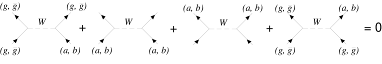
FIG. 2.: Cancellation among the scattering amplitudes in the ansatz of Equation (50) which do not preserve the number of particles in the shell ${\cal S}_{hf}$.

Taking these cancellations into account one obtains

$$W_{{\cal A}} := \frac{U}{4N}(g^{{\dagger}}_{\uparrow}+\bar{g}^{{\dagger}}_{\uparrow})(g^{{\dagger}}_{\downarrow}+\bar{g}^{{\dagger}}_{\downarrow})(g_{\downarrow}+\bar{g}_{\downarrow})(g_{\uparrow}+\bar{g}_{\uparrow})+$$ (61)

$$+ \frac{U}{2N}\sum_{i=1}^{N-1}\left[a^{{\dagger}}_{i\uparrow}(g^{{\dagger}}_{\downarrow}+\bar{g}^{{\dagger}}_{\downarrow})+(g^{{\dagger}}_{\uparrow}+\bar{g}^{{\dagger}}_{\uparrow})a^{{\dagger}}_{i\downarrow}\right]\left[(g_{\downarrow}+\bar{g}_{\downarrow})a_{i\uparrow}+a_{i\downarrow}(g_{\uparrow}+\bar{g}_{\uparrow})\right]$$ (62)

and

$$W_{{\cal B}} := \frac{U}{4N}(-g^{{\dagger}}_{\uparrow}+\bar{g}^{{\dagger}}_{\uparrow})(-g^{{\dagger}}_{\downarrow}+\bar{g}^{{\dagger}}_{\downarrow})(-g_{\downarrow}+\bar{g}_{\downarrow})(-g_{\uparrow}+\bar{g}_{\uparrow})+$$ (63)

$$+ \frac{U}{2N}\sum_{i=1}^{N-1}\left[b^{{\dagger}}_{i\uparrow}(-g^{{\dagger}}_{\downarrow}+\bar{g}^{{\dagger}}_{\downarrow})+(-g^{{\dagger}}_{\uparrow}+\bar{g}^{{\dagger}}_{\uparrow})b^{{\dagger}}_{i\downarrow}\right]\left[(-g_{\downarrow}+\bar{g}_{\downarrow})b_{i\uparrow}+b_{i\downarrow}(-g_{\uparrow}+\bar{g}_{\uparrow})\right]\;.$$ (64)

With $W$ written in the transformed picture one can calculate $W|\Psi_{0}(N,U)\rangle$. After very long, but standard algebra one finds

$$W|g^{0}\rangle\otimes|\Phi_{AF}^{0,0}\rangle = U\left\{\frac{2N-1}{2N}|g^{0}\rangle\otimes|\Phi_{AF}^{0,0}\rangle+\frac{1}{2N}|\bar{g}^{0}\rangle\otimes|\Phi_{AF}^{0,0}\rangle+\right.$$ (65)

$$+ \frac{1}{2N}\sum_{i=1}^{N-1}|[g\bar{g}]^{1,1}\rangle\otimes(-S^{-a}_{i}+S^{-b}_{i})|\Phi_{AF}^{0,0}\rangle+$$ (66)

$$+ \frac{1}{2N}\sum_{i=1}^{N-1}\left[\bar{g}^{{\dagger}}_{\uparrow}g^{{\dagger}}_{\downarrow}(\hat{n}^{a}_{i\downarrow}-n^{b}_{i\downarrow})+\bar{g}^{{\dagger}}_{\downarrow}g^{{\dagger}}_{\uparrow}(-\hat{n}^{a}_{i\uparrow}+n^{b}_{i\uparrow})\right]|\Phi_{AF}^{0,0}\rangle+$$ (67)

$$+ \left.\frac{1}{2N}\sum_{i=1}^{N-1}|[g\bar{g}]^{1,-1}\rangle\otimes(S^{+a}_{i}-S^{+b}_{i})|\Phi_{AF}^{0,0}\rangle\right\}$$ (68)

and

$$W|\bar{g}^{0}\rangle\otimes|\Phi_{AF}^{0,0}\rangle = U\left\{\frac{2N-1}{2N}|\bar{g}^{0}\rangle\otimes|\Phi_{AF}^{0,0}\rangle+\frac{1}{2N}|g^{0}\rangle\otimes|\Phi_{AF}^{0,0}\rangle+\right.$$ (69)

$$+ \frac{1}{2N}\sum_{i=1}^{N-1}|[g\bar{g}]^{1,1}\rangle\otimes(S^{-a}_{i}-S^{-b}_{i})|\Phi_{AF}^{0,0}\rangle+$$ (70)

$$+ \frac{1}{2N}\sum_{i=1}^{N-1}\left[g^{{\dagger}}_{\downarrow}\bar{g}^{{\dagger}}_{\uparrow}(-\hat{n}^{a}_{i\uparrow}+n^{b}_{i\uparrow})+g^{{\dagger}}_{\uparrow}\bar{g}^{{\dagger}}_{\downarrow}(\hat{n}^{a}_{i\downarrow}-n^{b}_{i\downarrow})\right]|\Phi_{AF}^{0,0}\rangle+$$ (71)

$$+ \left.\frac{1}{2N}\sum_{i=1}^{N-1}|[g\bar{g}]^{1,-1}\rangle\otimes(-S^{+a}_{i}+S^{+b}_{i})|\Phi_{AF}^{0,0}\rangle\right\}\;,$$ (72)

while for the singlet $\sum_{m=-1}^{1}(-)^{m}|[g\bar{g}]^{1,m}\rangle\otimes|\Phi_{AF}^{1,-m}\rangle$ one obtains

$$W\sum_{m=-1}^{1} (-)^{m} |[g\bar{g}]^{1,m}\rangle\otimes|\Phi_{AF}^{1,-m}\rangle=U\left\{\frac{N+1}{N}\sum_{m=-1}^{1}(-)^{m}|[g\bar{g}]^{1,m}\rangle\otimes|\Phi_{AF}^{1,-m}\rangle+\frac{1}{2N}(|g^{0}\rangle-|\bar{g}^{0}\rangle)\otimes\right.$$ (73)

$$\otimes \sum_{i=1}^{N-1}\left.\left[(S^{+a}_{i}-S^{+b}_{i})|\Phi_{AF}^{1,-1}\rangle+\frac{1}{\sqrt{2}}(n^{a}_{i\uparrow}-n^{a}_{i\downarrow}-n^{b}_{i\uparrow}+n^{b}_{i\downarrow})|\Phi_{AF}^{1,0}\rangle+(-S^{-a}_{i}+S^{-b}_{i})|\Phi_{AF}^{1,1}\rangle\right]\right\}\;.$$ (74)

By means of the identities in Eqs.(45-46-47) one can write Eqs.(68-72) in a compact form

$$W|g^{0}\rangle\otimes|\Phi_{AF}^{0,0}\rangle=U\left\{\frac{2N-1}{2N}|g^{0}\rangle\otimes|\Phi_{AF}^{0,0}\rangle+\frac{1}{2N}|\bar{g}^{0}\rangle\otimes|\Phi_{AF}^{0,0}\rangle+\frac{\sqrt{2}}{2N}\sum_{m=-1}^{1}(-)^{m}|[g\bar{g}]^{1,m}\rangle\otimes|\Phi_{AF}^{1,-m}\rangle\right\}$$ (75)

and

$$W|\bar{g}^{0}\rangle\otimes|\Phi_{AF}^{0,0}\rangle=U\left\{\frac{2N-1}{2N}|\bar{g}^{0}\rangle\otimes|\Phi_{AF}^{0,0}\rangle+\frac{1}{2N}|g^{0}\rangle\otimes|\Phi_{AF}^{0,0}\rangle-\frac{\sqrt{2}}{2N}\sum_{m=-1}^{1}(-)^{m}|[g\bar{g}]^{1,m}\rangle\otimes|\Phi_{AF}^{1,-m}\rangle\right\}\;.$$ (76)

Let us now consider the second row in Eq.(74). If our Ansatz is correct, the state in the square brackets must be proportional to $|\Phi_{AF}^{0,0}\rangle$. In this way one could close the equations and find an exact eigenstate. In Appendix B we prove that this is the case and in particular that

$$\sum_{i=1}^{N-1}\left[(S^{+a}_{i}-S^{+b}_{i})|\Phi_{AF}^{1,-1}\rangle+\frac{1}{\sqrt{2}}(n^{a}_{i\uparrow}-n^{a}_{i\downarrow}-n^{b}_{i\uparrow}+n^{b}_{i\downarrow})|\Phi_{AF}^{1,0}\rangle+(-S^{-a}_{i}+S^{-b}_{i})|\Phi_{AF}^{1,1}\rangle\right]=\sqrt{2}(N^{2}-1)|\Phi_{AF}^{0,0}\rangle\;.$$ (77)

Hence, Eq.(74) yields

$$W\sum_{m=-1}^{1}(-)^{m}|[g\bar{g}]^{1,m}\rangle\otimes|\Phi_{AF}^{1,-m}\rangle=U\left\{\frac{N+1}{N}\sum_{m=-1}^{1}(-)^{m}|[g\bar{g}]^{1,m}\rangle\otimes|\Phi_{AF}^{1,-m}\rangle+\right.$$ (78)

$$+\left.\sqrt{2}\frac{N^{2}-1}{2N}(|g^{0}\rangle-|\bar{g}^{0}\rangle)\otimes|\Phi_{AF}^{0,0}\rangle\right\}\;.$$ (79)

This result, together with Eqs.(75-76) and Eqs.(54), allows us to reduce the Schrodinger equation $(H_{{\mathrm{H}ubbard}}-E)|\Psi_{0}(N,U)\rangle=0$ to the diagonalization of the matrix

$$H(N,U)=\left(\begin{array}[]{ccc}-2t+\frac{2N-1}{2N}U&\frac{U}{2N}&\frac{\sqrt{2(N^{2}-1)}}{2N}U\\ &&\\ \frac{U}{2N}&2t+\frac{2N-1}{2N}U&-\frac{\sqrt{2(N^{2}-1)}}{2N}U\\ &&\\ \frac{\sqrt{2(N^{2}-1)}}{2N}U&-\frac{\sqrt{2(N^{2}-1)}}{2N}U&\frac{N+1}{N}U\end{array}\right)\;,$$ (80)

where the relations

$$\left[\langle g^{0}|\otimes\langle\Phi_{AF}^{0,0}|\right]\left[|g^{0}\rangle\otimes|\Phi_{AF}^{0,0}\rangle\right]=\left[\langle\bar{g}^{0}|\otimes\langle\Phi_{AF}^{0,0}|\right]\left[|\bar{g}^{0}\rangle\otimes|\Phi_{AF}^{0,0}\rangle\right]$$ (81)

and

$$\langle g^{0}|\otimes\langle\Phi_{AF}^{0,0}|W\sum_{m=-1}^{1}(-)^{m}|[g\bar{g}]^{1,m}\rangle\otimes|\Phi_{AF}^{1,-m}\rangle=\sum_{m=-1}^{1}(-)^{m}\langle\Phi_{AF}^{1,-m}|\otimes\langle[g\bar{g}]^{1,m}|W|g^{0}\rangle\otimes|\Phi_{AF}^{0,0}\rangle,$$ (82)

$$\langle\bar{g}^{0}|\otimes\langle\Phi_{AF}^{0,0}|W\sum_{m=-1}^{1}(-)^{m}|[g\bar{g}]^{1,m}\rangle\otimes|\Phi_{AF}^{1,-m}\rangle=\sum_{m=-1}^{1}(-)^{m}\langle\Phi_{AF}^{1,-m}|\otimes\langle[g\bar{g}]^{1,m}|W|\bar{g}^{0}\rangle\otimes|\Phi_{AF}^{0,0}\rangle$$ (83)

have been used to express $\sum_{m=-1}^{1}\langle\Phi_{AF}^{1,m}|\Phi_{AF}^{1,m}\rangle$ in terms of $\langle\Phi_{AF}^{0,0}|\Phi_{AF}^{0,0}\rangle$.

The thermodynamic limit $N\rightarrow\infty$ is well defined and non-trivial if we rescale $\tilde{t}$ in such a way that $N\tilde{t}=t=$const (which corresponds to the case of a fixed energy gap between the first two energy levels). The Hamiltonian matrix in Eq.(80) becomes

$$H(\infty,U)=\left(\begin{array}[]{ccc}-2t+U&0&U/\sqrt{2}\\ 0&2t+U&-U/\sqrt{2}\\ U/\sqrt{2}&-U/\sqrt{2}&U\end{array}\right)$$ (84)

with eigenvalues

$${\cal E}_{0}=U,\;\;\;{\cal E}_{\pm}=U\pm\Delta,\;\;\;\;\Delta\equiv\sqrt{U^{2}+4t^{2}}\;.$$ (85)

The (unnormalized) eigenvector corresponding to the lowest eigenvalue ${\cal E}_{-}$ gives

$$|\Psi_{0}(\infty,U)\rangle=\left[\left(\frac{U}{t}-\frac{2\Delta}{U}(2+\frac{\Delta}{t})\right)|g^{0}\rangle+\frac{U}{t}|\bar{g}^{0}\rangle\right]\otimes|\Phi_{AF}^{0,0}\rangle+\sqrt{2}(2+\frac{\Delta}{t})\sum_{m=-1}^{1}(-)^{m}|[g\bar{g}]^{1,m}\rangle\otimes|\Phi_{AF}^{1,-m}\rangle\;.$$ (86)

So far we have proved that the Ansatz in Eq.(50) gives three exact eigenstates of the CBG-Hubbard model at half filling. The eigenvalue of lowest energy ${\cal E}_{-}$ reduces to the non-interacting ground state energy for $U\rightarrow 0$, while the associated eigenstate (86) to the state $|g^{0}\rangle\otimes|\Phi_{AF}^{0,0}\rangle$. On the other hand, when $U\rightarrow\infty$ the original Hamiltonian can be mapped onto what we can define the CBG-Heisenberg Hamiltonian:

$$H_{{\mathrm{H}eisenberg}}=\frac{4\tilde{t}^{2}}{U}\sum_{x\in{\cal A}}\sum_{y\in{\cal B}}({\mathbf{S}}_{x}\cdot{\mathbf{S}}_{y}-\frac{1}{4})\;.$$ (87)

This model is exactly solvable and the ground state is obtained by projecting onto the singlet the state where $N$ particles lie on the ${\cal A}$-sites with spin up and the remaining $N$ on the ${\cal B}$-sites with spin down (Neel state): one finds

$$|\Psi_{0}(N,\infty)\rangle=\sum_{P}(-)^{P}\prod_{x=1}^{N}\sigma^{{\dagger}}_{x,P(x+N)}|0\rangle$$ (88)

with $\sigma^{{\dagger}}_{x,y}=\frac{1}{\sqrt{2}}(c^{{\dagger}}_{x\uparrow}c^{{\dagger}}_{y\downarrow}-c^{{\dagger}}_{x\downarrow}c^{{\dagger}}_{y\uparrow})$. The ground state energy is $-2t^{2}/U$ for $N\rightarrow\infty$ and is equal to the first order approximation of ${\cal E}_{-}$ in the small parameter $(t/U)^{2}$ (the same conclusion holds for any finite $N$, although it is more tedious to prove). Furthermore, by direct inspection of the lowest energy eigenvector of $H(N,U)$ one can show that $|\Psi_{0}(N,U)\rangle$ becomes the state in Eq.(88) when $U\rightarrow\infty$. Therefore, $|\Psi_{0}(N,U)\rangle$ reduces to the ground state of the CBG-Hubbard model in the two opposite limits $U\rightarrow 0$ and $U\rightarrow\infty$.

To prove that the lowest energy eigenstate of $H(N,U)$ is the unique ground state we are looking for, one can exploit the ground state uniqueness of the Heisenberg Hamiltonian proved in Ref.[26]. Since $|\Psi_{0}(N,\infty)\rangle$ is the ground state of the Heisenberg model and since the ground state of the half-filled Hubbard model is unique, a level crossing for some value of $U$ would be required if $|\Psi_{0}(N,U)\rangle$ were an excited state, contradicting the uniqueness.

In conclusion we have proved that the Ansatz in Eq.(50) with $(\gamma_{g},\gamma_{\bar{g}},\gamma_{0})$ given by the lowest energy eigenvector of the matrix in Eq.(80) is the exact ground state of the half-filled Hubbard model defined on the CBG of size $|\Lambda|=2N$ and repulsion $U$. In the next Section we shall calculate some physical quantities, as the spin-spin correlation function, and we shall prove that the particles are antiferromagnetically ordered.

VI Results and Discussion

The exact ground state solution for arbitrary but finite $N$ allows to study the ground state energy $E_{0}(N,U)$ as a function of $N$ and $U$. Taking $\tilde{t}N=t=1$, in Fig.(3) we have plotted $E_{0}(N,U)$ in the range $N=1,..,10$ and $0<U<20$.

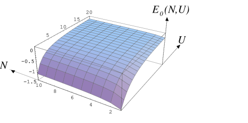
FIG. 3.: Ground state energy $E_{0}(N,U)$ of the half-filled Hubbard model on the CBG as a function of the on-site repulsion parameter $U$ and the number of lattice sites $N$ in each sublattice. The hopping parameter has been chosen to be $t=1$.

The figure shows that $E_{0}(N,U)$ is a monotonically increasing function of $N$ and $U$, that is $E_{0}(N+1,U)-E_{0}(N)>0$ and $\partial E_{0}(N,U)/\partial U>0$. The limit $N\rightarrow\infty$ at fixed $U$ is given by ${\cal E}_{-}$ in Eq.(85):

$$\lim_{|\Lambda|\rightarrow\infty}\lim_{\beta\rightarrow\infty}E^{(\beta)}(|\Lambda|,t,U)=U-\sqrt{U^{2}+4t^{2}}<0$$ (89)

where $E^{(\beta)}(|\Lambda|,t,U)$ is the internal energy of the system at inverse Temperature $\beta$ and number of lattice sites $|\Lambda|=2N$. On the other hand, one can calculate the internal energy at zero Temperature in thermodynamic limit: $E^{(\beta)}(|\Lambda|\rightarrow\infty,t,U)=\Omega_{\beta}+k_{B}S/\beta+\mu|\Lambda|n$ with $\Omega_{\beta}$ from Eq.(23) and $S$ the entropy. Following the procedure of van Dongen and Vollhardt one gets

$$\lim_{\beta\rightarrow\infty}\lim_{|\Lambda|\rightarrow\infty}E^{(\beta)}(|\Lambda|,t,U)=\left\{\begin{array}[]{ll}-2t=-2N\tilde{t}<0&{\mathrm{i}f}\;\tilde{t}\;{\mathrm{i}s}\;{\mathrm{n}ot}\;{\mathrm{r}escaled}\\ O(1)&{\mathrm{i}f}\;\tilde{t}\sim 1/|\Lambda|\end{array}\right.\;.$$ (90)

In the case $\tilde{t}$=const the two limits commute and the trivial thermodynamic behavior of the model originates from the infinite gap between the lowest level and the zero-energy levels: the two particles in the $g$ orbitals are completely decoupled from the dynamics of the system. On the other hand, if $\tilde{t}$ is rescaled the gap remains frozen and taking $|\Lambda|\rightarrow\infty$ first, we can only say that the ground state energy is $O(1)$, but we cannot predict the exact amount within the scheme proposed by van Dongen and Vollhardt. This is a consequence of the fact that in the limit $|\Lambda|\rightarrow\infty$, we retain only the extensive contributions to the internal energy.

The ground state energy Eq.(89) is always higher than that of the non-interacting case and hence non-trivial correlations survive in the thermodynamic limit. To understand the nature of these correlations we have calculated the ground state average of the number of doubly occupied sites:

$$\overline{D}(N,U)\equiv\frac{\overline{W}(N,U)}{U}\equiv\frac{1}{U}\langle\Psi_{0}(N,U)|W|\Psi_{0}(N,U)\rangle = \frac{1}{U}\langle\Psi_{0}(N,U)|H_{{\mathrm{H}ubbard}}-H_{0}|\Psi_{0}(N,U)\rangle=$$ (91)

$$= \frac{1}{U}E_{0}(N,U)+\frac{2t}{U}[\gamma^{2}_{g}(N,U)-\gamma^{2}_{{\bar{g}}}(N,U)]$$ (92)

where $\gamma_{g}$ and $\gamma_{{\bar{g}}}$ are the first two components of the normalized ground state vector, see Eq.(50). In Fig.(4$a$) we have plotted the trend of $\overline{D}(N,U)$ as $N$ increases for different values of $U$. As expected $\overline{D}(N,U)$ is a monotonically decreasing function of $U$, $\partial\overline{D}(N,U)/\partial U<0$, approaching zero for $U\rightarrow\infty$ [where the exact ground state reduces to the antiferromagnetic Neel state, see Eq.(88)]. Nevertheless, $\overline{D}(N,U)$ shows a non-trivial behaviour as $N$ increases at fixed $U$ values. In the weak coupling regime, $U\ll t$, the number of doubly occupied sites grows as $N$ becomes larger and larger converging to a finite value when $N\rightarrow\infty$. The opposite trend is observed in the strong coupling regime, $U\gg t$, where $\overline{D}(N,U)$ decreases as $N$ increases. In the intermediate regime $U\sim t$, $\overline{D}(N,U)$ is an increasing function of $N$ for small $N$, but becomes an decreasing function for large $N$. Hence, there is a critical value $U_{c}(N)$ where the analytic continuation of $\overline{D}(N,U)$ to real $N$ verifies

$$\left(\frac{\partial^{2}\overline{D}}{\partial U\partial N}\right)_{U_{c}(N)}=0$$ (93)

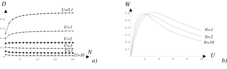
FIG. 4.: $a$) Trend of the ground state average of the number of doubly occupied sites versus $N$ in the range $1\leq N\leq 20$ for different values of the Hubbard interaction parameter $U=$0.1, 1, 2, 3, 5, 10. $b$) Ground state average of the interaction term $W$ as a function of $U$ in the range $0\leq U\leq 10$ for three different number of sublattice sites, $N=$ 1, 2, 10. The hopping parameter has been chosen to be $t=1$ in both cases.

In Fig.(4$b$) we report the ground state average of the interacting term $W$ as a function of $U$ for three different values of $N$. There is always a critical value for $U$ where the repulsion is maximized. Moreover, $\lim_{N\rightarrow\infty}\overline{W}(N,U)\equiv\overline{W}_{\infty}(U)\neq 0$ for any finite $U$ and the system cannot avoid double occupation neither in the thermodynamic limit. In the limit $U\rightarrow\infty$, $\overline{W}(N,U)\rightarrow 0$ according to the Gutzwiller Ansatz[27].

Next, we have calculated the spin-spin correlation function

$$G_{{\mathrm{s}pin}}(x,y)\equiv\langle\Psi_{0}(N,U)|S^{z}_{x}S^{z}_{y}|\Psi_{0}(N,U)\rangle=\lim_{\beta\rightarrow\infty}G_{{\mathrm{s}pin}}(x,y;\beta,h=0,|\Lambda|)=\lim_{\beta\rightarrow\infty}\lim_{h\rightarrow 0}G_{{\mathrm{s}pin}}(x,y;\beta,h,|\Lambda|)$$ (94)

where $G_{{\mathrm{s}pin}}(x,y;\beta,h,|\Lambda|)$ was defined in Section III, $S^{z}_{x}=\frac{1}{2}(\hat{n}_{x\uparrow}-\hat{n}_{x\downarrow})$ and $|\Psi_{0}\rangle$ is the normalized ground state

$$|\Psi_{0}\rangle=\left[\frac{\gamma_{g}}{{\cal N}_{0}}|g^{0}\rangle+\frac{\gamma_{\bar{g}}}{{\cal N}_{0}}|\bar{g}^{0}\rangle\right]\otimes|\Phi_{AF}^{0,0}\rangle+\frac{1}{\sqrt{3}}\frac{\gamma_{0}}{{\cal N}_{1}}\sum_{m=-1}^{1}(-)^{m}|[g\bar{g}]^{1,m}\rangle\otimes|\Phi_{AF}^{1,-m}\rangle\;,$$ (95)

with ${\cal N}^{2}_{0}=\langle\Phi_{AF}^{0,0}|\Phi_{AF}^{0,0}\rangle$, ${\cal N}^{2}_{1}=\langle\Phi_{AF}^{1,m}|\Phi_{AF}^{1,m}\rangle$, $m=0,\pm 1$, and $\gamma_{g}^{2}+\gamma_{\bar{g}}^{2}+\gamma_{0}^{2}=1$. Due to the $S_{N}\otimes S_{N}\otimes Z_{2}$ symmetry, $G_{{\mathrm{s}pin}}(x,y)$ can be written as

$$G_{{\mathrm{s}pin}}(x,y)=\left\{\begin{array}[]{ll}G_{0}&x=y\\ G_{{\mathrm{o}n}}&x\in{\cal A}\;(x\in{\cal B})\;{\mathrm{a}nd}\;y\in{\cal A}\;(y\in{\cal B})\\ G_{{\mathrm{o}ff}}&x\in{\cal A}\;(x\in{\cal B})\;{\mathrm{a}nd}\;y\in{\cal B}\;(x\in{\cal A})\end{array}\right.$$ (96)

and by exploiting the sum rule $\sum_{y\in\Lambda}G_{{\mathrm{s}pin}}(x,y)=G_{0}+(N-1)G_{{\mathrm{o}n}}+NG_{{\mathrm{o}ff}}=0$, one can express $G_{{\mathrm{o}n}}$ in terms of $G_{{\mathrm{o}ff}}$ and $G_{0}$:

$$G_{{\mathrm{o}n}}=-\frac{N}{N-1}G_{{\mathrm{o}ff}}-\frac{G_{0}}{N-1}\;.$$ (97)

The problem is then reduced to the evaluation of $G_{0}$ and $G_{{\mathrm{o}ff}}$. We have

$$G_{0} = G_{{\mathrm{s}pin}}(x,x)=\langle\Psi_{0}|(S^{z}_{x})^{2}|\Psi_{0}\rangle=\frac{1}{2N}\sum_{x\in\Lambda}\langle\Psi_{0}|(S^{z}_{x})^{2}|\Psi_{0}\rangle=$$ (98)

$$= \frac{1}{8N}\sum_{x\in\Lambda}\langle\Psi_{0}|\hat{n}_{x\uparrow}+\hat{n}_{x\downarrow}-2\hat{n}_{x\uparrow}\hat{n}_{x\downarrow}|\Psi_{0}\rangle=\frac{1}{4}(1-\frac{\overline{D}}{N})\;.$$ (99)

More effort is needed to calculate $G_{{\mathrm{o}ff}}$. Expanding the $c$ operators in $g$, ${\bar{g}}$, $a$ and $b$ operators of Eq.(12) and taking into account that $(\sum_{x\in\Lambda}S^{z}_{x})^{2}|\Psi_{0}\rangle=0$, we get

$$G_{{\mathrm{o}ff}}=-\frac{1}{N^{2}}\sum_{x\in{\cal A}}\sum_{y\in{\cal A}}\langle\Psi_{0}|S^{z}_{x}S^{z}_{y}|\Psi_{0}\rangle=-\frac{1}{N^{2}}\left[\frac{1}{16}\langle\Psi_{0}|\left(\sum_{\sigma}(-)^{\sigma}(g^{{\dagger}}_{\sigma}+\bar{g}^{{\dagger}}_{\sigma})(g_{\sigma}+\bar{g}_{\sigma})\right)^{2}|\Psi_{0}\rangle\right.+$$ (100)

$$+\left.\frac{1}{2}\langle\Psi_{0}|S^{za}\sum_{\sigma}(-)^{\sigma}(g^{{\dagger}}_{\sigma}+\bar{g}^{{\dagger}}_{\sigma})(g_{\sigma}+\bar{g}_{\sigma})|\Psi_{0}\rangle+\langle\Psi_{0}|S^{za}S^{za}|\Psi_{0}\rangle\right]$$ (101)

with $(-)^{\sigma}=+,-$ for $\sigma=\uparrow,\downarrow$. After long but standard algebra one obtains

$$G_{{\mathrm{o}ff}}=-\frac{1}{N^{2}}\left\{\frac{1}{8}\left[(\gamma_{g}-\gamma_{{\bar{g}}})^{2}+2\gamma_{0}^{2}\right]-\sqrt{\frac{2}{3}}\frac{\gamma_{0}(\gamma_{g}-\gamma_{{\bar{g}}})}{{\cal N}_{0}{\cal N}_{1}}\langle\Phi_{AF}^{1,0}|S^{za}|\Phi_{AF}^{0,0}\rangle+\frac{\gamma_{g}^{2}+\gamma^{2}_{{\bar{g}}}}{{\cal N}_{0}^{2}}\langle\Phi_{AF}^{0,0}|S^{za}S^{za}|\Phi_{AF}^{0,0}\rangle+\right.$$ (102)

$$+\left.\frac{\gamma_{0}^{2}}{3{\cal N}_{1}^{2}}\left[\langle\Phi_{AF}^{1,-1}|S^{za}|\Phi_{AF}^{1,-1}\rangle-\langle\Phi_{AF}^{1,1}|S^{za}|\Phi_{AF}^{1,1}\rangle+\sum_{m=-1}^{1}\langle\Phi_{AF}^{1,m}|S^{za}S^{za}|\Phi_{AF}^{1,m}\rangle\right]\right\}\;.$$ (103)

and exploiting the $Z_{2}$ symmetry $a_{i}\rightarrow b_{i}$ and $b_{i}\rightarrow a_{i}$, which implies $|\Phi_{AF}^{S,M_{S}}\rangle\rightarrow(-)^{S}|\Phi_{AF}^{S,M_{S}}\rangle$,

$$\langle\Phi_{AF}^{1,0}|S^{za}|\Phi_{AF}^{0,0}\rangle=-\langle\Phi_{AF}^{1,0}|S^{zb}|\Phi_{AF}^{0,0}\rangle=\frac{1}{2}\langle\Phi_{AF}^{1,0}|S^{za}-S^{zb}|\Phi_{AF}^{0,0}\rangle=\frac{1}{2}{\cal N}_{1}^{2}$$ (104)

$$\langle\Phi_{AF}^{1,1}|S^{za}|\Phi_{AF}^{1,1}\rangle=\frac{1}{2}\langle\Phi_{AF}^{1,1}|S^{za}+S^{zb}|\Phi_{AF}^{1,1}\rangle=\frac{1}{2}{\cal N}_{1}^{2}$$ (105)

$$\langle\Phi_{AF}^{1,-1}|S^{za}|\Phi_{AF}^{1,-1}\rangle=\frac{1}{2}\langle\Phi_{AF}^{1,-1}|S^{za}+S^{zb}|\Phi_{AF}^{1,-1}\rangle=-\frac{1}{2}{\cal N}_{1}^{2}$$ (106)

where in Eq.(104) we have used the identity Eq.(46). Finally we recall that the $W=0$ states $|\Phi_{AF}^{S,M_{S}}\rangle$ are eigenstates of the square of the total spin operators of each sublattice $S^{2}_{{\cal A}}\equiv(S^{za})^{2}+\frac{1}{2}(S^{+a}S^{-a}+S^{-a}S^{+a})$ and $S^{2}_{{\cal B}}\equiv(S^{zb})^{2}+\frac{1}{2}(S^{+b}S^{-b}+S^{-b}S^{+b})$ with eigenvalue $(\frac{N-1}{2})(\frac{N-1}{2}+1)=\frac{1}{4}(N^{2}-1)$; hence

$$\sum_{M_{S}=-S}^{S}\langle\Phi_{AF}^{S,M_{S}}|(S^{za})^{2}|\Phi_{AF}^{S,M_{S}}\rangle=\frac{N^{2}-1}{12}(2S+1){\cal N}^{2}_{S};\;\;\;\;{\cal N}^{2}_{S}=\langle\Phi_{AF}^{S,M_{S}}|\Phi_{AF}^{S,M_{S}}\rangle,\;\;M_{S}=-S,\ldots,S\;.$$ (107)

Substitution of Eqs.(104-105-106-107) in Eq.(103) yields

$$G_{{\mathrm{o}ff}}=-\frac{1}{N^{2}}\left\{\frac{N^{2}-1}{12}+\frac{1}{8}[(\gamma_{g}-\gamma_{{\bar{g}}})^{2}+2\gamma_{0}^{2}]-\frac{1}{3}\gamma_{0}^{2}-\sqrt{\frac{N^{2}-1}{18}}\gamma_{0}(\gamma_{g}-\gamma_{{\bar{g}}})\right\}$$ (108)

where we have taken into account Eq.(83) to evaluate the ratio ${\cal N}_{1}/{\cal N}_{0}=\sqrt{(N^{2}-1)/3}$.

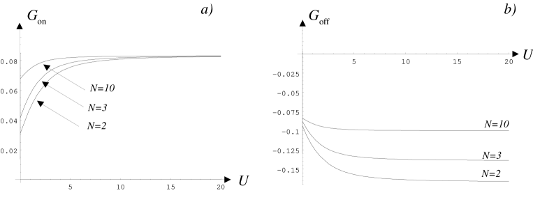
FIG. 5.: $a$) $G_{{\mathrm{o}n}}$ versus $U$ in the range $0\leq U\leq 20$ for three different values of the number of sites $N=2,\;3,\;10$. $b$) $G_{{\mathrm{o}ff}}$ versus $U$ in the range $0\leq U\leq 20$ for three different values of the number of sites $N=2,\;3,\;10$. The hopping parameter has been chosen to be $t=1$ in both cases.

In Fig.(5) we report the trend of $G_{{\mathrm{o}n}}$ and $G_{{\mathrm{o}ff}}$ versus $U$ for three different values of $N=2,\;3,\;10$. According to the Shen-Qiu-Tian theorem[28], $G_{{\mathrm{o}n}}$ is always larger than zero while $G_{{\mathrm{o}ff}}$ is always negative. Now consider the ground state average of the square of the staggered magnetization operator

$$m^{2}_{AF}\equiv\frac{1}{|\Lambda|}\langle\Psi_{0}|[\sum_{x\in\Lambda}\epsilon(x)S^{z}_{x}]^{2}|\Psi_{0}\rangle,\;\;\;\;\epsilon(x)=1,\;-1\;{\mathrm{f}or}\;\;x\in{\cal A},\;{\cal B}\;.$$ (109)

The Shen-Qiu-Tian theorem implies that each term in the expansion of Eq.(109) is non-negative. We emphasize, however, that for $|{\cal A}|=|{\cal B}|$ this does not imply that $m^{2}_{AF}$ is an extensive quantity! Remarkably, our results show that $m^{2}_{AF}=G_{0}+(N-1)G_{{\mathrm{o}n}}-NG_{{\mathrm{o}ff}}$ is extensive for any value of the on-site repulsion parameter $U$ and provide an example of antiferromagnetism in the ground state of an itinerant-electrons model of arbitrary size.

We also observe that the thermodynamic limit yields a non-vanishing result:

$$\lim_{|\Lambda|\rightarrow\infty}G_{0}=\frac{1}{4},\;\;\;\;\lim_{|\Lambda|\rightarrow\infty}G_{{\mathrm{o}n}}=-\lim_{|\Lambda|\rightarrow\infty}G_{{\mathrm{o}ff}}=\frac{1}{12},\;\;\;\;$$ (110)

or

$$\lim_{|\Lambda|\rightarrow\infty}\lim_{\beta\rightarrow\infty}\lim_{h\rightarrow 0}|G_{{\mathrm{s}pin}}(x,y;\beta,h,|\Lambda|)|=\frac{1}{12}\;\;\;{\mathrm{f}or}\;x\neq y\;.$$ (111)

By comparing Eq.(111) with Eq.(30), we see that the $\lim_{\beta\rightarrow\infty}\lim_{h\rightarrow 0}$ do not commute with the $\lim_{|\Lambda|\rightarrow\infty}$.

VII Summary and Conclusions

We have introduced the CBG-Hubbard model and explicitly written the ground state wave function at half filling for any repulsion parameter $U$. The topology of the graph $\Lambda$ allows $(2N-2)$-body eigenstates $|\Phi_{AF}^{S,M_{S}}\rangle$ of the Hamiltonian which are free of double occupation. They can be obtained projecting the determinantal state $|\Phi_{AF}\rangle$ on a given spin-$S$ subspace. $|\Phi_{AF}\rangle$ has the antiferromagnetic property, that is the map ${\cal A}\leftrightarrow{\cal B}$ is equivalent to a spin-flip.

We have shown that the ground state has a fixed number of particles in the zero-energy one-body shell ${\cal S}_{hf}$, independent of $t$ and $U$. This very remarkable Shell Population Rigidity holds in any finite-size system and it provides the closure of the equations. This implies extra-conservation laws in a suitable subspace of the full Hilbert space including the ground state. Only the singlet $|\Phi_{AF}^{0,0}\rangle$ and the triplet $|\Phi_{AF}^{1,m}\rangle$, $m=0,\pm 1$, are involved in the ground state expansion. Qualitatively, we may say that according to Eq.(86) the particles in the shell ${\cal S}_{hf}$ manage to avoid the double occupation.

We have calculated the spin-spin correlation function and shown that the ground state exhibits an antiferromagnetic order for any non-zero $U$ even in the thermodynamic limit. The kinetic term induces non-trivial correlations among the particles and an antiparallel spin configuration in the two sublattices turns out to be energetically favoured. Therefore, the model contains the basic ingredients to understand how the subtle competition between the delocalization induced by $H_{0}$ and the localization induced by $W$ may give rise to a magnetically ordered state even outside the strong coupling regime (where the Hubbard model is equivalent to the Heisenberg model). On the other hand, within the scheme proposed by van Dongen and Vollhardt, the model is well described by a paramagnetic Hamiltonian; the difference stems from taking the thermodynamic limit before the limit of zero Temperature, because then the kinetic term completly decouples from the interaction and loses any r$\hat{o}$le in the physical response functions.

The present formalism lends itself to solve more realistic Hubbard Hamiltonians with an increasing number of negative and positive energy levels. Higher-spin projections $|\Phi_{AF}^{S,M_{S}}\rangle$ are involved in the ground state expansions; the results will be published elsewhere. We are currently investigating group-theory aspects of this model and its extensions.

Finally, we recall[23][24][25] that the standard Hubbard model on a $N\times N$ square lattice and periodic boundary conditions also has $|\Phi_{AF}^{S,M_{S}}\rangle$-like eigenstates. It could be that the Shell Population Rigidity holds in this case too, but the proof is lacking.

A Shell Population Rigidity

We have seen in Section V that the most part of the contributions which do not preserve the number of particles in the shell ${\cal S}_{hf}$ yield nothing. To prove the Shell Popoulation Rigidity property we need to show that the sequences like $a^{{\dagger}}a^{{\dagger}}ga$ and similar terms with $b$ instead of $a$ and/or $g$ replaced by $\bar{g}$ vanish or in formulæ

$$\sum_{x\in{\cal A}}\sum_{ijm}R_{i,x}R_{j,x}R_{m,x}a^{{\dagger}}_{i\uparrow}a^{{\dagger}}_{j\downarrow}a_{m\sigma}|\Phi_{AF}^{S,M_{S}}\rangle=0$$ (A1)

and the like with $a$ replaced by $b$. This last spectacular cancellation can be seen by particle-hole transforming Eq.(A1). Under a particle-hole transformation $c_{x\sigma}\rightarrow c^{{\dagger}}_{x\sigma}$ and the $W=0$ states $|\Phi_{AF}^{S,M_{S}}\rangle\rightarrow|g^{0}\bar{g}^{0}\rangle\otimes|\Phi_{AF}^{S,-M_{S}}\rangle$, modulo a phase factor. Hence, Eq.(A1) is equivalent to

$$\sum_{x\in{\cal A}}\sum_{ijm}R_{i,x}R_{j,x}R_{m,x}a_{i\uparrow}a_{j\downarrow}a^{{\dagger}}_{m\sigma}|\Phi_{AF}^{S,M_{S}}\rangle=0\;.$$ (A2)

Let the spin of the operator $a^{{\dagger}}_{m\sigma}$ be up for the sake of definiteness (the same reasoning holds in the case of down spin). The l.h.s. of Eq.(A2) can be rewritten as

$$-\sum_{x\in{\cal A}}\sum_{ijm}R_{i,x}R_{j,x}R_{m,x}[\delta_{i,m}-a^{{\dagger}}_{m\uparrow}a_{i\uparrow}]a_{j\downarrow}|\Phi_{AF}^{S,M_{S}}\rangle=-\sum_{j}\left[\sum_{x}\sum_{i}R^{2}_{i,x}R_{j,x}\right]a_{j\downarrow}|\Phi_{AF}^{S,M_{S}}\rangle$$ (A3)

where we have exploited the lack of double occupation of the $W=0$ state, see Eq.(55). Therefore, we are left to prove that

$$\sum_{x=1}^{N}\sum_{i=1}^{N-1}R_{j,x}R^{2}_{i,x}=0,\;\;\;\forall j\;.$$ (A4)

We recall that $R$ is an $(N-1)\times N$ rectangular matrix whose rows are orthonormal vectors which are orthogonal to the $N-$dimensional vector $(1,1,\ldots,1,1)$. It is a simple exercise to verify that

$$R=\left(\begin{array}[]{cccccc}\frac{1}{\sqrt{2}}&-\frac{1}{\sqrt{2}}&0&0&\ldots&0\\ \frac{1}{\sqrt{6}}&\frac{1}{\sqrt{6}}&-\frac{2}{\sqrt{3}}&0&\ldots&0\\ :&:&:&:&:&:\\ \frac{1}{\sqrt{N(N+1)}}&\frac{1}{\sqrt{N(N+1)}}&\frac{1}{\sqrt{N(N+1)}}&\frac{1}{\sqrt{N(N+1)}}&\ldots&-\sqrt{\frac{N}{(N+1)}}\end{array}\right)\;\Rightarrow R_{m,x}=\left\{\begin{array}[]{ll}0&x>m+1\\ -\sqrt{\frac{m}{m+1}}&x=m+1\\ \frac{1}{m}\sqrt{\frac{m}{m+1}}&x\leq m\end{array}\right.$$ (A5)

is a correct choice and that Eq.(A4) is identically verified.

B Proof of Eq.(77)

To prove Eq.(77) we shall use the definitions (36-42-43) for the triplet $W=0$ state $|\Phi_{AF}^{1,m}\rangle$, $m=0,\pm 1$. The first term yields

$$\sum_{k}(S^{+a}_{k}-S^{+b}_{k})|\Phi_{AF}^{1,-1}\rangle = \sum_{P}(-)^{P}\sum_{k}(S^{+a}_{k}-S^{+b}_{P(k)})\sum_{j}\tau^{(-1)^{{\dagger}}}_{j,P(j)}\prod_{i\neq j}\sigma^{{\dagger}}_{i,P(i)}|0\rangle=$$ (B1)

$$= \sum_{P}(-)^{P}\sum_{j}(S^{+a}_{j}-S^{+b}_{P(j)})\tau^{(-1)^{{\dagger}}}_{j,P(j)}\prod_{i\neq j}\sigma^{{\dagger}}_{i,P(i)}|0\rangle+$$ (B2)

$$+ \sum_{P}(-)^{P}\sum_{j}\tau^{(-1)^{{\dagger}}}_{j,P(j)}\sum_{k\neq j}(S^{+a}_{k}-S^{+b}_{P(k)})\sigma^{{\dagger}}_{k,P(k)}\prod_{i\neq j,k}\sigma^{{\dagger}}_{i,P(i)}|0\rangle=$$ (B3)

$$= \sqrt{2}\sum_{P}(-)^{P}\sum_{j}\sigma^{{\dagger}}_{j,P(j)}\prod_{i\neq j}\sigma^{{\dagger}}_{i,P(i)}|0\rangle+$$ (B4)

$$- \sqrt{2}\sum_{P}(-)^{P}\sum_{j}\sum_{k\neq j}\tau^{(-1)^{{\dagger}}}_{j,P(j)}\tau^{(+1)^{{\dagger}}}_{k,P(k)}\prod_{i\neq j,k}\sigma^{{\dagger}}_{i,P(i)}|0\rangle=$$ (B5)

$$= \sqrt{2}(N-1)|\Phi_{AF}^{0,0}\rangle-\sqrt{2}\sum_{P}(-)^{P}\sum_{j}\sum_{k\neq j}\tau^{(-1)^{{\dagger}}}_{j,P(j)}\tau^{(+1)^{{\dagger}}}_{k,P(k)}\prod_{i\neq j,k}\sigma^{{\dagger}}_{i,P(i)}|0\rangle\;,$$ (B6)

while second term yields

$$\sum_{k}(\hat{n}^{a}_{k\uparrow}-\hat{n}^{a}_{k\downarrow} - \hat{n}^{b}_{k\uparrow}+\hat{n}^{b}_{k\downarrow})|\Phi_{AF}^{1,0}\rangle=\sum_{P}(-)^{P}\sum_{k}(\hat{n}^{a}_{k\uparrow}-\hat{n}^{a}_{k\downarrow}-\hat{n}^{b}_{P(k)\uparrow}+\hat{n}^{b}_{P(k)\downarrow})\sum_{j}\tau^{(0)^{{\dagger}}}_{j,P(j)}\prod_{i\neq j}\sigma^{{\dagger}}_{i,P(i)}|0\rangle=$$ (B7)

$$= \sum_{P}(-)^{P}\sum_{j}(\hat{n}^{a}_{j\uparrow}-\hat{n}^{a}_{j\downarrow}-\hat{n}^{b}_{P(j)\uparrow}+\hat{n}^{b}_{P(j)\downarrow})\tau^{(0)^{{\dagger}}}_{j,P(j)}\prod_{i\neq j}\sigma^{{\dagger}}_{i,P(i)}|0\rangle+$$ (B8)

$$+ \sum_{P}(-)^{P}\sum_{j}\tau^{(0)^{{\dagger}}}_{j,P(j)}\sum_{k\neq j}(\hat{n}^{a}_{k\uparrow}-\hat{n}^{a}_{k\downarrow}-\hat{n}^{b}_{P(k)\uparrow}+\hat{n}^{b}_{P(k)\downarrow})\sigma^{{\dagger}}_{k,P(k)}\prod_{i\neq j,k}\sigma^{{\dagger}}_{i,P(i)}|0\rangle=$$ (B9)

$$= 2\sum_{P}(-)^{P}\sum_{j}\sigma^{{\dagger}}_{j,P(j)}\prod_{i\neq j}\sigma^{{\dagger}}_{i,P(i)}|0\rangle+$$ (B10)

$$+ 2\sum_{P}(-)^{P}\sum_{j}\sum_{k\neq j}\tau^{(0)^{{\dagger}}}_{j,P(j)}\tau^{(0)^{{\dagger}}}_{k,P(k)}\prod_{i\neq j,k}\sigma^{{\dagger}}_{i,P(i)}|0\rangle=$$ (B11)

$$= 2(N-1)|\Phi_{AF}^{0,0}\rangle+2\sum_{P}(-)^{P}\sum_{j}\sum_{k\neq j}\tau^{(0)^{{\dagger}}}_{j,P(j)}\tau^{(0)^{{\dagger}}}_{k,P(k)}\prod_{i\neq j,k}\sigma^{{\dagger}}_{i,P(i)}|0\rangle\;.$$ (B12)

The third term can be computed following the same steps of Eq.(B6) and the final result is

$$\sum_{k}(-S^{-a}_{k}+S^{-b}_{k})|\Phi_{AF}^{1,1}\rangle=\sqrt{2}(N-1)|\Phi_{AF}^{0,0}\rangle-\sqrt{2}\sum_{P}(-)^{P}\sum_{j}\sum_{k\neq j}\tau^{(+1)^{{\dagger}}}_{j,P(j)}\tau^{(-1)^{{\dagger}}}_{k,P(k)}\prod_{i\neq j,k}\sigma^{{\dagger}}_{i,P(i)}|0\rangle\;.$$ (B13)

Denoting by $[..]$ the left hand side of Eq.(77), from Eqs.(B6-B12-B13) one obtains

$$[..]=3\sqrt{2}(N-1)|\Phi_{AF}^{0,0}\rangle-\sqrt{2}\sum_{P}(-)^{P}\sum_{j}\sum_{k\neq j}\left[\tau^{(-1)^{{\dagger}}}_{j,P(j)}\tau^{(+1)^{{\dagger}}}_{k,P(k)}-\tau^{(0)^{{\dagger}}}_{j,P(j)}\tau^{(0)^{{\dagger}}}_{k,P(k)}+\tau^{(+1)^{{\dagger}}}_{j,P(j)}\tau^{(-1)^{{\dagger}}}_{k,P(k)}\right]\prod_{i\neq j,k}\sigma^{{\dagger}}_{i,P(i)}|0\rangle.$$ (B14)

(B15)

Let us consider the first and the third term in the square bracket of the right hand side of Eq.(B15). We have

$$\sum_{P^{\prime}}(-)^{P^{\prime}}\left[\tau^{(-1)^{{\dagger}}}_{j,P^{\prime}(j)}\tau^{(+1)^{{\dagger}}}_{k,P^{\prime}(k)}+\tau^{(+1)^{{\dagger}}}_{j,P^{\prime}(j)}\tau^{(-1)^{{\dagger}}}_{k,P^{\prime}(k)}\right]\prod_{i\neq j,k}\sigma^{{\dagger}}_{i,P^{\prime}(i)}|0\rangle=$$ (B16)

$$=-\sum_{P}(-)^{P}\left[\tau^{(-1)^{{\dagger}}}_{j,P(k)}\tau^{(+1)^{{\dagger}}}_{k,P(j)}+\tau^{(+1)^{{\dagger}}}_{j,P(k)}\tau^{(-1)^{{\dagger}}}_{k,P(j)}\right]\prod_{i\neq j,k}\sigma^{{\dagger}}_{i,P(i)}|0\rangle$$ (B17)

where the permutations $P$ and $P^{\prime}$ satisfy

$$P^{\prime}(k)=P(j),\;\;\;\;P^{\prime}(j)=P(k),\;\;\;\;P^{\prime}(i)=P(i)\;\;\forall i\neq j,k\;;$$ (B18)

hence $(-)^{P^{\prime}}=-(-)^{P}$. Substituting Eq.(B17) into Eq.(B15) and taking into account that

$$\tau^{(-1)^{{\dagger}}}_{j,P(k)}\tau^{(+1)^{{\dagger}}}_{k,P(j)}+\tau^{(0)^{{\dagger}}}_{j,P(j)}\tau^{(0)^{{\dagger}}}_{k,P(k)}+\tau^{(+1)^{{\dagger}}}_{j,P(k)}\tau^{(-1)^{{\dagger}}}_{k,P(j)}=\sigma^{{\dagger}}_{j,P(j)}\sigma^{{\dagger}}_{k,P(k)}$$ (B19)

one obtains

$$[..]=3\sqrt{2}(N-1)|\Phi_{AF}^{0,0}\rangle+\sqrt{2}\sum_{P}(-)^{P}\sum_{j}\sum_{k\neq j}\sigma^{{\dagger}}_{j,P(j)}\sigma^{{\dagger}}_{k,P(k)}\prod_{i\neq j,k}\sigma^{{\dagger}}_{i,P(i)}|0\rangle=\sqrt{2}(N^{2}-1)|\Phi_{AF}^{0,0}\rangle\;,$$ (B20)

that is, Eq.(77).

REFERENCES

REFERENCES

- [1] E. H. Lieb and F. Y. Wu, Phys. Rev. Lett. 20, 1445 (1968).
- [2] H. A. Bethe, Zeits. f. Phys. 71, 205 (1931); E. H. Lieb and W. Liniger, Phys. Rev. 130, 1605 (1963).
- [3] J. B. McGuire, J. Math. Phys. 6, 432 (1965); M. Flicker and E. H. Lieb, Phys. Rev. 161, 179 (1967).
- [4] C. N. Yang, Phys. Rev. Lett. 19, 1312 (1967); M. Gaudin, Phys. Letters A 24, 55 (1967).
- [5] Gang Su, Bao-Heng Zhao and Mo-Liu Ge, Phys. Rev. B 46, 14909 (1992).
- [6] You-Quou Li and Christian Gruber, Phys. Rev. Lett. 80, 1034 (1998).
- [7] Boyu Hou, Dantao Peng and Ruihong Yue, cond-mat/0010485 (2000).
- [8] E. H. Lieb, Phys. Rev. Lett. 62, 1201 (1989).
- [9] Y. Nagaoka Phys. Rev. 147, 392 (1966).
- [10] A. Mielke J. Phys A 24, L73 (1991); A. Mielke J. Phys A 25, 4335 (1992); A. Mielke Phys. Lett. A 174, 443 (1993); A. Mielke Phys. Rev. Lett. 82, 4312 (1999); A. Mielke, J. Phys A 32, 8411 (1999).
- [11] H. Tasaki Phys. Rev. Lett. 69, 1608 (1992); H. Tasaki J. Stat. Phys. 84, 535 (1996).
- [12] D. F. Wang, cond-mat/9604121.
- [13] J. D. Patterson, Phys. Rev. B 6, 1041 (1972).
- [14] P. van Dongen and D. Vollhardt, Phys. Rev. B 40, 7252 (1989).
- [15] J. A. Verges, F. Guinea, J. Galan, P. van Dongen, G. Chiappe and E. Louis, Phys. Rev. B 49, 15400 (1994).
- [16] U. Brandt and A. Giesekus, Phys. Rev. Lett. 68, 2648 (1992).
- [17] A. Mielke, J. Phys. A 24, 3311 (1991); A. Mielke and H. Tasaki, Commun. Math. Phys. 158, 341 (1993).
- [18] O.J. Heilmann and E. H. Lieb, Annals N.Y. Acad. Sci. 172, 583 (1971).
- [19] Cheng Ning Yang, Phys. Rev. Lett. 63, 2144 (1989).
- [20] Cheng Ning Yang and S. C. Zhang, Mod. Phys. Lett. B 4, 759 (1990).
- [21] There is a simple trick to see that the number of independent wavefunctions obtained in this way is . Let be a permutation such that and . We get the full basis since takes values with independent .
- [22] At weak coupling it makes sense to speak about particles in filled shells, which behave much as core electrons in atomic physics, and particles in partially filled, or valence, shells. In first order, we must diagonalize the perturbation in the degenerate subspace, dropping the filled shells. Since is a positive semi-definite operator, with vanishing eigenvalue, 0 is necessarily the lowest one. Typically, the first-order solution is a crude approximation to the exact one, but below, when discussing the exact results, we shall demonstrate that many of the qualitative features hold for all .
- [23] Michele Cini and Gianluca Stefanucci, Solid State Communications 117, 451 (2001).
- [24] Michele Cini and Gianluca Stefanucci, J. Phys.: Condens. Matter 13, 1279 (2001).
- [25] Gianluca Stefanucci and Michele Cini, J. Phys.: Condens. Matter 14, 2653 (2002).
- [26] E. H. Lieb and D. C. Mattis, J. Math. Phys. 3, 749 (1962).
- [27] M. C. Gutzwiller, Phys. Rev. Lett. 10, 159 (1963).
- [28] S. Q. Shen, Z. M. Qiu and G. S. Tian, Phys. Rev. Lett. 72, 1280 (1994).