Random graphs as models of networks

Abstract

The random graph of Erdős and Rényi is one of the oldest and best studied models of a network, and possesses the considerable advantage of being exactly solvable for many of its average properties. However, as a model of real-world networks such as the Internet, social networks or biological networks it leaves a lot to be desired. In particular, it differs from real networks in two crucial ways: it lacks network clustering or transitivity, and it has an unrealistic Poissonian degree distribution. In this paper we review some recent work on generalizations of the random graph aimed at correcting these shortcomings. We describe generalized random graph models of both directed and undirected networks that incorporate arbitrary non-Poisson degree distributions, and extensions of these models that incorporate clustering too. We also describe two recent applications of random graph models to the problems of network robustness and of epidemics spreading on contact networks.

1 Introduction

In a series of seminal papers in the 1950s and 1960s, Paul Erdős and Alfréd Rényi proposed and studied one of the earliest theoretical models of a network, the random graph (Erdős and Rényi, 1959, 1960, 1961). This minimal model consists of $n$ nodes or vertices, joined by links or edges which are placed between pairs of vertices chosen uniformly at random. Erdős and Rényi gave a number of versions of their model. The most commonly studied is the one denoted $G_{n,p}$, in which each possible edge between two vertices is present with independent probability $p$, and absent with probability $1-p$. Technically, in fact, $G_{n,p}$ is the ensemble of graphs of $n$ vertices in which each graph appears with the probability appropriate to its number of edges.

Often one wishes to express properties of $G_{n,p}$ not in terms of $p$ but in terms of the average degree $z$ of a vertex. (The degree of a vertex is the number of edges connected to that vertex.) The average number of edges on the graph as a whole is $\mbox{$\frac{1}{2}$}n(n-1)p$, and the average number of ends of edges is twice this, since each edge has two ends. So the average degree of a vertex is

$$z={n(n-1)p\over n}=(n-1)p\simeq np,$$ (1)

where the last approximate equality is good for large $n$. Thus, once we know $n$, any property that can be expressed in terms of $p$ can also be expressed in terms of $z$.

The Erdős–Rényi random graph has a number of desirable properties as a model of a network. In particular it is found that many of its ensemble average properties can be calculated exactly in the limit of large $n$ (Bollobás, 1985; Janson et al., 1999). For example, one interesting feature, which was demonstrated in the original papers by Erdős and Rényi, is that the model shows a phase transition with increasing $z$ at which a giant component forms. A component is a subset of vertices in the graph each of which is reachable from the others by some path through the network. For small values of $z$, when there are few edges in the graph, it is not surprising to find that most vertices are disconnected from one another, and components are small, having an average size that remains constant as the graph becomes large. However, there is a critical value of $z$ above which the one largest component in the graph contains a finite fraction $S$ of the total number of vertices, i.e., its size $nS$ scales linearly with the size of the whole graph. This largest component is the giant component. In general there will be other components in addition to the giant component, but these are still small, having an average size that remains constant as the graph grows larger. The phase transition at which the giant component forms occurs precisely at $z=1$. If we regard the fraction $S$ of the graph occupied by the largest component as an order parameter, then the transition falls in the same universality class as the mean-field percolation transition (Stauffer and Aharony, 1992).

The formation of a giant component in the random graph is reminiscent of the behaviour of many real-world networks. One can imagine loose-knit networks for which there are so few edges that, presumably, the network has no giant component, and all vertices are connected to only a few others. The social network in which pairs of people are connected if they have had a conversation within the last 60 seconds, for example, is probably so sparse that it has no giant component. The network in which people are connected if they have ever had a conversation, on the other hand, is very densely connected and certainly has a giant component.

However, the random graph differs from real-world networks in some fundamental ways also. Two differences in particular have been noted in the recent literature (Strogatz, 2001; Albert and Barabási, 2002). First, as pointed out by Watts and Strogatz (1998; Watts 1999) real-world networks show strong clustering or network transitivity, where Erdős and Rényi’s model does not. A network is said to show clustering if the probability of two vertices being connected by an edge is higher when the vertices in question have a common neighbour. That is, there is another vertex in the network to which they are both attached. Watts and Strogatz measured this clustering by defining a clustering coefficient $C$, which is the average probability that two neighbours of a given vertex are also neighbours of one another. In many real-world networks the clustering coefficient is found to have a high value, anywhere from a few percent to 50 percent or even more. In the random graph of Erdős and Rényi on the other hand, the probabilities of vertex pairs being connected by edges are by definition independent, so that there is no greater probability of two vertices being connected if they have a mutual neighbour than if they do not. This means that the clustering coefficient for a random graph is simply $C=p$, or equivalently $C\simeq z/n$. In Table 1 we compare clustering coefficients for a number of real-world networks with their values on a random graph with the same number of vertices and edges. The graphs listed in the table are:

			clustering coefficient $C$
network	$n$	$z$	measured	random graph
Internet (autonomous systems)a	$6\,374$	$3.8$	$0.24$	$0.00060$
World-Wide Web (sites)b	$153\,127$	$35.2$	$0.11$	$0.00023$
power gridc	$4\,941$	$2.7$	$0.080$	$0.00054$
biology collaborationsd	$1\,520\,251$	$15.5$	$0.081$	$0.000010$
mathematics collaborationse	$253\,339$	$3.9$	$0.15$	$0.000015$
film actor collaborationsf	$449\,913$	$113.4$	$0.20$	$0.00025$
company directorsf	$7\,673$	$14.4$	$0.59$	$0.0019$
word co-occurrenceg	$460\,902$	$70.1$	$0.44$	$0.00015$
neural networkc	$282$	$14.0$	$0.28$	$0.049$
metabolic networkh	$315$	$28.3$	$0.59$	$0.090$
food webi	$134$	$8.7$	$0.22$	$0.065$

Table 1: Number of vertices $n$, mean degree $z$, and clustering coefficient $C$ for a number of different networks. Numbers are taken from ^aPastor-Satorras et al. (2001), ^bAdamic (1999), ^cWatts and Strogatz (1998), ^dNewman (2001b), ^eNewman (2001d), ^fNewman et al. (2001), ^gi Cancho and Solé (2001), ^hFell and Wagner (2000), ⁱMontoya and Solé (2002).

• Internet: a graph of the fibre optic connections that comprise the Internet, at the level of so-called “autonomous systems.” An autonomous system is a group of computers within which data flow is handled autonomously, while data flow between groups is conveyed over the public Internet. Examples of autonomous systems might be the computers at a company, a university, or an Internet service provider.

• World-Wide Web: a graph of sites on the World-Wide Web in which edges represent “hyperlinks” connecting one site to another. A site in this case means a collection of pages residing on a server with a given name. Although hyperlinks are directional, their direction has been ignored in this calculation of the clustering coefficient.

• Power grid: a graph of the Western States electricity transmission grid in the United States. Vertices represent stations and substations; edges represent transmission lines.

• Biology collaborations: a graph of collaborations between researchers working in biology and medicine. A collaboration between two scientists is defined in this case as coauthorship of a paper that was catalogued in the Medline bibliographic database between 1995 and 1999 inclusive.

• Mathematics collaborations: a similar collaboration graph for mathematicians, derived from the archives of Mathematical Reviews.

• Film actor collaborations: a graph of collaborations between film actors, where a collaboration means that the two actors in question have appeared in a film together. The data are from the Internet Movie Database.

• Company directors: a collaboration graph of the directors of companies in the Fortune 1000 for 1999. (The Fortune 1000 is the 1000 US companies with the highest revenues during the year in question.) Collaboration in this case means that two directors served on the board of a Fortune 1000 company together.

• Word co-occurrences: a graph in which the vertices represent words in the English language, and an edge signifies that the vertices it connects frequently occur in adjacent positions in sentences.

• Neural network: a graph of the neural network of the worm C. Elegans.

• Metabolic network: a graph of interactions forming a part of the energy generation and small building block synthesis metabolism of the bacterium E. Coli. Vertices represent substrates and products, and edges represent interactions.

• Food web: the food web of predator–prey interactions between species in Ythan Estuary, a marine estuary near Aberdeen, Scotland. Like the links in the World-Wide Web graph, the directed nature of the interactions in this food web have been neglected for the purposes of calculating the clustering coefficient.

As the table shows, the agreement between the clustering coefficients in the real networks and in the corresponding random graphs is not good. The real and theoretical figures differ by as much as four orders of magnitude in some cases. Clearly, the random graph does a poor job of capturing this particular property of networks.

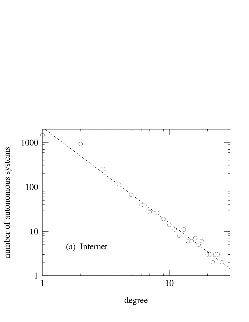
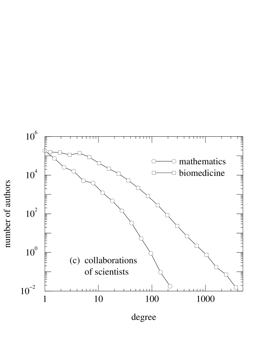
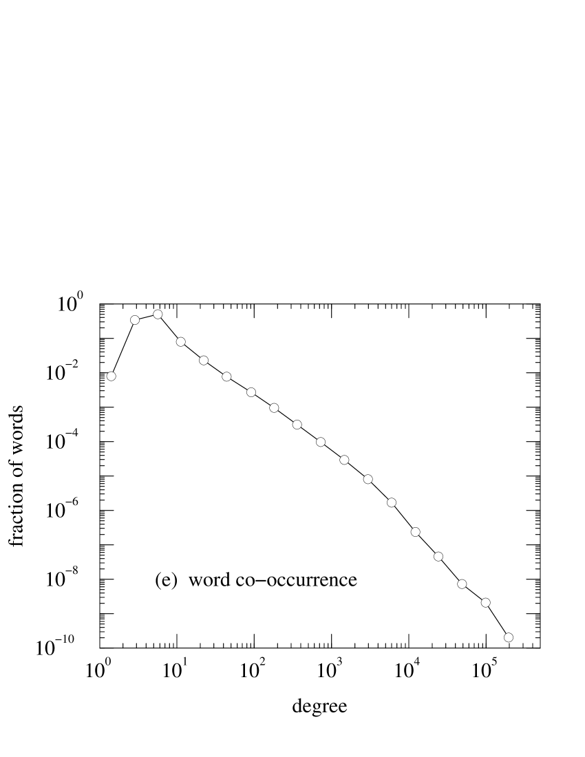
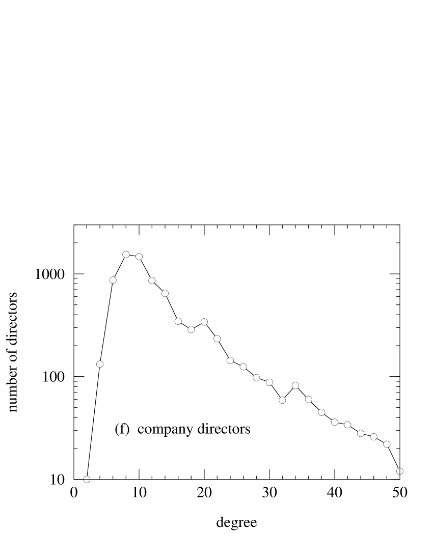
Figure 1: Measured degree distributions for a number of different networks. (a) Physical connections between autonomous systems on the Internet, circa 1997 (Faloutsos et al., 1999). (b) A 200 million page subset of the World-Wide Web, circa 1999 (Broder et al., 2000). The figure shows the out-degree of pages, i.e., numbers of links pointing from those pages to other pages. (c) Collaborations between biomedical scientists and between mathematicians (Newman, 2001b, d). (d) Collaborations of film actors (Amaral et al., 2000). (e) Co-occurrence of words in the English language (i Cancho and Solé, 2001). (f) Board membership of directors of Fortune 1000 companies for year 1999 (Newman et al., 2001).

A second way in which random graphs differ from their real-world counterparts is in their degree distributions, a point which has been emphasized particularly in the work of Albert, Barabási, and collaborators (Albert et al., 1999; Barabási and Albert, 1999). The probability $p_{k}$ that a vertex in an Erdős–Rényi random graph has degree exactly $k$ is given by the binomial distribution:

$$p_{k}={n-1\choose k}p^{k}(1-p)^{n-1-k}.$$ (2)

In the limit where $n\gg kz$, this becomes

$$p_{k}={z^{k}{\rm e}^{-z}\over k!},$$ (3)

which is the well-known Poisson distribution. Both binomial and Poisson distributions are strongly peaked about the mean $z$, and have a large-$k$ tail that decays rapidly as $1/k!$. We can compare these predictions to the degree distributions of real networks by constructing histograms of the degrees of vertices in the real networks. We show some examples, taken from the networks described above, in Fig. 1. As the figure shows, in most cases the degree distribution of the real network is very different from the Poisson distribution. Many of the networks, including Internet and World-Wide Web graphs, appear to have power-law degree distributions (Albert et al., 1999; Faloutsos et al., 1999; Broder et al., 2000), which means that a small but non-negligible fraction of the vertices in these networks have very large degree. This behaviour is quite unlike the rapidly decaying Poisson degree distribution, and can have profound effects on the behaviour of the network, as we will see later in this paper. Other networks, particularly the collaboration graphs, appear to have power-law degree distributions with an exponential cutoff at high degree (Amaral et al., 2000; Newman, 2001a, b), while others still, such as the graph of company directors, seem to have degree distributions with a purely exponential tail (Newman et al., 2001). The power grid of Table 1 is another example of a network that has an exponential degree distribution (Amaral et al., 2000).

In this paper we show how to generalize the Erdős–Rényi random graph to mimic the clustering and degree properties of real-world networks. In fact, most of the paper is devoted to extensions that correct the degree distribution, for which an elegant body of theory has been developed in the last few years. However, towards the end of the paper we also consider ways in which clustering can be introduced into random graphs. Work on this latter problem is significantly less far advanced than work on degree distributions, and we have at present only a few preliminary results. Whether these results can be extended, and how, are open questions.

2 Random graphs with specified degree distributions

It is relatively straightforward to generate random graphs that have non-Poisson degree distributions. The method for doing this has been discussed a number of times in the literature, but appears to have been put forward first by Bender and Canfield (1978). The trick is to restrict oneself to a specific degree sequence, i.e., to a specified set $\{k_{i}\}$ of the degrees of the vertices $i=1\ldots n$. Typically this set will be chosen in such a way that the fraction of vertices having degree $k$ will tend to the desired degree distribution $p_{k}$ as $n$ becomes large. For practical purposes however, such as numerical simulation, it is almost always adequate simply to draw a degree sequence $\{k_{i}\}$ from the distribution $p_{k}$ directly.

Once one has one’s degree sequence, the method for generating the graph is as follows: one gives each vertex $i$ a number $k_{i}$ of “stubs”—ends of edges emerging from the vertex—and then one chooses pairs of these stubs uniformly at random and joins them together to make complete edges. When all stubs have been used up, the resulting graph is a random member of the ensemble of graphs with the desired degree sequence. Note that, because of the $k_{i}!$ possible permutations of the stubs emerging from the $i$th vertex, there are $\prod_{i}k_{i}!$ different ways of generating each graph in the ensemble. However, this factor is constant so long as the degree sequence $\{k_{i}\}$ is held fixed, so it does not prevent the method from sampling the ensemble correctly. This is the reason why we restrict ourselves to a fixed degree sequence—merely fixing the degree distribution is not adequate to ensure that the method described here generates graphs uniformly at random from the desired ensemble.

The method of Bender and Canfield does not allow us to specify a clustering coefficient for our graph. (The clustering coefficient had not been invented yet when Bender and Canfield were writing in 1978.) Indeed the fact that the clustering coefficient is not specified is one of the crucial properties of these graphs that makes it possible, as we will show, to solve exactly for many of their properties in the limit of large graph size. As an example of why this is important, consider the following simple calculation. The mean number of neighbours of a randomly chosen vertex A in a graph with degree distribution $p_{k}$ is $z=\langle k\rangle=\sum_{k}kp_{k}$. Suppose however that we want to know the mean number of second neighbours of vertex A, i.e., the mean number of vertices two steps away from A in the graph. In a network with clustering, many of the second neighbours of a vertex are also first neighbours—the friend of my friend is also my friend—and we would have to allow for this effect to order avoid overcounting the number of second neighbours. In our random graphs however, no allowances need be made. The probability that one of the second neighbours of A is also a first neighbour goes as $n^{-1}$ in the random graph, regardless of degree distribution, and hence can be ignored in the limit of large $n$.

There is another effect, however, that we certainly must take into account if we wish to compute correctly the number of second neighbours: the degree distribution of the first neighbour of a vertex is not the same as the degree distribution of vertices on the graph as a whole. Because a high-degree vertex has more edges connected to it, there is a higher chance that any given edge on the graph will be connected to it, in precise proportion to the vertex’s degree. Thus the probability distribution of the degree of the vertex to which an edge leads is proportional to $kp_{k}$ and not just $p_{k}$ (Feld, 1991; Molloy and Reed, 1995; Newman, 2001d). This distinction is absolutely crucial to all the further developments of this paper, and the reader will find it worthwhile to make sure that he or she is comfortable with it before continuing.

In fact, we are interested here not in the complete degree of the vertex reached by following an edge from A, but in the number of edges emerging from such a vertex other than the one we arrived along, since the latter edge only leads back to vertex A and so does not contribute to the number of second neighbours of A. This number is one less than the total degree of the vertex and its correctly normalized distribution is therefore $q_{k-1}=kp_{k}/\sum_{j}jp_{j}$, or equivalently

$$q_{k}={(k+1)p_{k+1}\over\sum_{j}jp_{j}}.$$ (4)

The average degree of such a vertex is then

$$\sum_{k=0}^{\infty}kq_{k}={\sum_{k=0}^{\infty}k(k+1)p_{k+1}\over\sum_{j}jp_{j}}={\sum_{k=0}^{\infty}(k-1)kp_{k}\over\sum_{j}jp_{j}}={\langle k^{2}\rangle-\langle k\rangle\over\langle k\rangle}.$$ (5)

This is the average number of vertices two steps away from our vertex A via a particular one of its neighbours. Multiplying this by the mean degree of A, which is just $z=\langle k\rangle$, we thus find that the mean number of second neighbours of a vertex is

$$z_{2}=\langle k^{2}\rangle-\langle k\rangle.$$ (6)

If we evaluate this expression using the Poisson degree distribution, Eq. (3), then we get $z_{2}=\langle k\rangle^{2}$—the mean number of second neighbours of a vertex in an Erdős–Rényi random graph is just the square of the mean number of first neighbours. This is a special case however. For most degree distributions Eq. (6) will be dominated by the term $\langle k^{2}\rangle$, so the number of second neighbours is roughly the mean square degree, rather than the square of the mean. For broad distributions such as those seen in Fig. 1, these two quantities can be very different (Newman, 2001d).

We can extend this calculation to further neighbours also. The average number of edges leading from each second neighbour, other than the one we arrived along, is also given by (5), and indeed this is true at any distance $m$ away from vertex A. Thus the average number of neighbours at distance $m$ is

$$z_{m}={\langle k^{2}\rangle-\langle k\rangle\over\langle k\rangle}z_{m-1}={z_{2}\over z_{1}}z_{m-1},$$ (7)

where $z_{1}\equiv z=\langle k\rangle$ and $z_{2}$ is given by Eq. (6). Iterating this equation we then determine that

$$z_{m}=\biggl{[}{z_{2}\over z_{1}}\biggr{]}^{m-1}z_{1}.$$ (8)

Depending on whether $z_{2}$ is greater than $z_{1}$ or not, this expression will either diverge or converge exponentially as $m$ becomes large, so that the average total number of neighbours of vertex A at all distances is finite if $z_{2}<z_{1}$ or infinite if $z_{2}>z_{1}$ (in the limit of infinite $n$). If this number is finite, then clearly there can be no giant component in the graph. Conversely, if it is infinite, then there must be a giant component. Thus the graph shows a phase transition similar to that of the Erdős–Rényi graph precisely at the point where $z_{2}=z_{1}$. Making use of Eq. (6) and rearranging, we find that this condition is also equivalent to $\langle k^{2}\rangle-2\langle k\rangle=0$, or, as it is more commonly written,

$$\sum_{k=0}^{\infty}k(k-2)p_{k}=0.$$ (9)

This condition for the position of the phase transition in a random graph with arbitrary degree sequence was first given by Molloy and Reed (1995).

An interesting feature of Eq. (9) is that, because of the factor $k(k-2)$, vertices of degree zero and degree two contribute nothing to the sum, and therefore the number of such vertices does not affect the position of the phase transition or the existence of the giant component. It is easy to see why this should be the case for vertices of degree zero; obviously one can remove (or add) degree-zero vertices without changing the fact of whether a giant component does or does not exist in a graph. But why vertices of degree two? This has a simple explanation also: removing vertices of degree two does not change the topological structure of a graph because all such vertices fall in the middle of edges between other pairs of vertices. We can therefore remove (or add) any number of such vertices without affecting the existence of the giant component.

Another quantity of interest in many networks is the typical distance through the network between pairs of vertices (Milgram, 1967; Travers and Milgram, 1969; Pool and Kochen, 1978; Watts and Strogatz, 1998; Amaral et al., 2000). We can use Eq. (8) to make a calculation of this quantity for our random graph as follows. If we are “below” the phase transition of Eq. (9), in the regime where there is no giant component, then most pairs of vertices will not be connected to one another at all, so vertex–vertex distance has little meaning. Well above the transition on the other hand, where there is a giant component, all vertices in this giant component are connected by some path to all others. Eq. (8) tells us the average number of vertices a distance $m$ away from a given vertex A in the giant component. When the total number of vertices within distance $m$ is equal to the size $n$ of the whole graph, $m$ is equal to the so-called “radius” $r$ of the network around vertex A. Indeed, since $z_{2}/z_{1}\gg 1$ well above the transition, the number of vertices at distance $m$ grows quickly with $m$ in this regime (see Eq. (8) again), which means that most of the vertices in the network will be far from A, around distance $r$, and $r$ is thus also approximately equal to the average vertex–vertex distance $\ell$. Well above the transition therefore, $\ell$ is given approximately by $z_{\ell}\simeq n$, or

$$\ell={\log(n/z_{1})\over\log(z_{2}/z_{1})}+1.$$ (10)

For the special case of the Erdős–Rényi random graph, for which $z_{1}=z$ and $z_{2}=z^{2}$ as noted above, this expression reduces to the well-known standard formula for this case: $\ell=\log n/\log z$ (Bollobás, 1985).

The important point to notice about Eq. (10) is that the vertex–vertex distance increases logarithmically with the graph size $n$, i.e., it grows rather slowly. Even for very large networks we expect the typical distance through the network from one vertex to another to be quite small. In social networks this effect is known as the small-world effect, and was famously observed by the experimental psychologist Stanley Milgram in the letter-passing experiments he conducted in the 1960s (Milgram, 1967; Travers and Milgram, 1969; Kleinfeld, 2000). More recently it has been observed also in many other networks including non-social networks (Watts and Strogatz, 1998; Amaral et al., 2000). This should come as no great surprise to us however. On the contrary, it would be surprising if most networks did not show the small-world effect. If we define the diameter $d$ of a graph to be the maximum distance between any two connected vertices in the graph, then it can be proven rigorously that the fraction of all possible graphs with $n$ vertices and $m$ edges for which $d>c\log n$ for some constant $c$ tends to zero as $n$ becomes large (Bollobás, 1985). And clearly if the diameter increases as $\log n$ or slower, then so also must the average vertex–vertex distance. Thus our chances of finding a network that does not show the small-world effect are very small for large $n$.

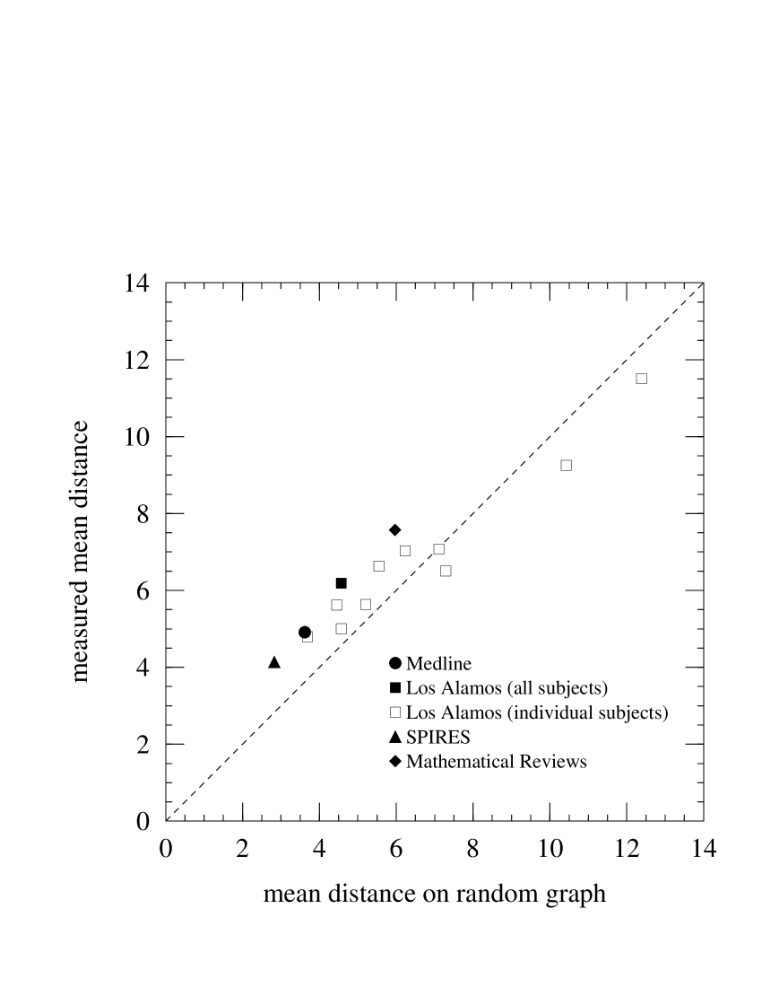
Figure 2: Comparison of mean vertex–vertex distance measured in fourteen collaboration networks against our theoretical predictions of the same quantities from Eq. (10). The networks are constructed using bibliographic data for papers in biology and medicine (Medline), physics (Los Alamos E-print Archive), high-energy physics (SPIRES), and mathematics (Mathematical Reviews). If empirical results and theory agreed perfectly, the points would fall on the dotted diagonal line. After Newman (2001c).

As a test of Eq. (10), Fig. 2 compares our predictions of average distance $\ell$ with direct measurements for fourteen different scientific collaboration networks, including the biology and mathematics networks of Table 1. In this figure, each network is represented by a single point, whose position along the horizontal axis corresponds to the theoretically predicted value of $\ell$ and along the vertical axis the measured value. If Eq. (10) were exactly correct, all the points in the figure would fall on the dotted diagonal line. Since we know that the equation is only approximate, it comes as no surprise that the points do not fall perfectly along this line, but the results are encouraging nonetheless; in most cases the theoretical prediction is close to the correct result and the overall scaling of $\ell$ with $\log n$ is clear. If the theory were equally successful for networks of other types, it would provide a useful way of estimating average vertex–vertex separation. Since $z_{1}$ and $z_{2}$ are local quantities that can be calculated at least approximately from measurements on only a small portion of the network, it would in many cases be considerably simpler and more practical to apply Eq. (10) than to measure $\ell$ directly.

Although our random graph model does not allow us to fix the level of clustering in the network, we can still calculate an average clustering coefficient for the Bender–Canfield ensemble easily enough. Consider a particular vertex A again. The $i$th neighbour of A has $k_{i}$ edges emerging from it other than the edge attached to A, and $k_{i}$ is distributed according to the distribution $q_{k}$, Eq. (4). The probability that this vertex is connected to another neighbour $j$ is $k_{i}k_{j}/(nz)$, where $k_{j}$ is also distributed according to $q_{k}$, and average of this probability is precisely the clustering coefficient:

$$C={\langle k_{i}k_{j}\rangle\over nz}={1\over nz}\,\Bigl{[}\sum_{k}kq_{k}\Bigr{]}^{2}={z\over n}\,\biggl{[}{\langle k^{2}\rangle-\langle k\rangle\over\langle k\rangle^{2}}\biggr{]}^{2}={z\over n}\,\biggl{[}c_{v}^{2}+{z-1\over z}\biggr{]}^{2}.$$ (11)

The quantity $c_{v}$ is the so-called coefficient of variation of the degree distribution—the ratio of the standard deviation to the mean. Thus the clustering coefficient for the random graph with a non-Poisson degree distribution is equal to its value $z/n$ for the Poisson-distributed case, times a function whose leading term goes as the fourth power of the coefficient of variation of the degree distribution. So the clustering coefficient still vanishes with increasing graph size, but may have a much larger leading coefficient, since $c_{v}$ can be quite large, especially for degree distributions with long tails, such as those seen in Fig. 1.

Take for example the World-Wide Web. If one ignores the directed nature of links on the Web, then the resulting graph is measured to have quite a high clustering coefficient of $0.11$ (Adamic, 1999), as shown in Table 1. The Erdős–Rényi random graph with the same $n$ and $z$, by contrast, has a clustering coefficient of only $0.00023$. However, if we use the degree distribution shown in Fig. 1a to calculate a mean degree and coefficient of variation for the Web, we get $z=10.23$ and $c_{v}=3.685$, which means that $(c_{v}^{2}+(z-1)/z)^{2}=209.7$. Eq. (11) then tells us that the random graph with the correct degree distribution would actually have a clustering coefficient of $C=0.00023\times 209.7=0.048$. This is still about a factor of two away from the correct answer, but a lot closer to the mark than the original estimate, which was off by a factor of more than 400. Furthermore, the degree distribution used in this calculation was truncated at $k=4096$. (The data were supplied to author in this form.) Without this truncation, the coefficient of variation would presumably be larger still. It seems possible therefore, that most, if not all, of the clustering seen in the Web can be accounted for merely as a result of the long-tailed degree distribution. Thus the fact that our random graph models do not explicitly include clustering is not necessarily a problem.

On the other hand, some of the other networks of Table 1 do show significantly higher clustering than would be predicted by Eq. (11). For these, our random graphs will be an imperfect model, although as we will see they still have much to contribute. Extension of our models to include clustering explicitly is discussed in Section 6.

It would be possible to continue the analysis of our random graph models using the simple methods of this section. However, this leads to a lot of tedious algebra which can be avoided by introducing an elegant tool, the probability generating function.

3 Probability generating functions

In this section we describe the use of probability generating functions to calculate the properties of random graphs. Our presentation closely follows that of Newman et al. (2001).

A probability generating function is an alternative representation of a probability distribution. Take the probability distribution $p_{k}$ introduced in the previous section, for instance, which is the distribution of vertex degrees in a graph. The corresponding generating function is

$$G_{0}(x)=\sum_{k=0}^{\infty}p_{k}x^{k}.$$ (12)

It is clear that this function captures all of the information present in the original distribution $p_{k}$, since we can recover $p_{k}$ from $G_{0}(x)$ by simple differentiation:

$$p_{k}={1\over k!}{{\rm d}^{k}G_{0}\over{\rm d}x^{k}}\bigg{|}_{x=0}.$$ (13)

We say that the function $G_{0}$ “generates” the probability distribution $p_{k}$.

We can also define a generating function for the distribution $q_{k}$, Eq. (4), of other edges leaving the vertex we reach by following an edge in the graph:

$$G_{1}(x)=\sum_{k=0}^{\infty}q_{k}x^{k}={\sum_{k=0}^{\infty}(k+1)p_{k+1}x^{k}\over\sum_{j}jp_{j}}={\sum_{k=0}^{\infty}kp_{k}x^{k-1}\over\sum_{j}jp_{j}}={G_{0}^{\prime}(x)\over z},$$ (14)

where $G_{0}^{\prime}(x)$ denotes the first derivative of $G_{0}(x)$ with respect to its argument. This generating function will be useful to us in following developments.

3.1 Properties of generating functions

Generating functions have some properties that will be of use in this paper. First, if the distribution they generate is properly normalized then

$$G_{0}(1)=\sum_{k}p_{k}=1.$$ (15)

Second, the mean of the distribution can be calculated directly by differentiation:

$$G^{\prime}_{0}(1)=\sum_{k}kp_{k}=\langle k\rangle.$$ (16)

Indeed we can calculate any moment of the distribution by taking a suitable derivative. In general,

$$\langle k^{n}\rangle=\sum_{k}k^{n}p_{k}=\biggl{[}\biggl{(}x{{\rm d}\over{\rm d}x}\biggr{)}^{\!n}G_{0}(x)\biggr{]}_{x=1}.$$ (17)

Third, and most important, if a generating function generates the probability distribution of some property $k$ of an object, such as the degree of a vertex, then the sum of that property over $n$ independent such objects is distributed according to the $n$th power of the generating function. Thus the sum of the degrees of $n$ randomly chosen vertices on our graph has a distribution which is generated by the function $[G_{0}(x)]^{n}$. To see this, note that the coefficient of $x^{m}$ in $[G_{0}(x)]^{n}$ has one term of the form $p_{k_{1}}p_{k_{2}}\ldots p_{k_{n}}$ for every set $\{k_{i}\}$ of the degrees of the $n$ vertices such that $\sum_{i}k_{i}=m$. But these terms are precisely the probabilities that the degrees sum to $m$ in every possible way, and hence $[G_{0}(x)]^{n}$ is the correct generating function. This property is the reason why generating functions are useful in the study of random graphs. Most of the results of this paper rely on it.

3.2 Examples

To make these ideas more concrete, let us consider some specific examples of generating functions. Suppose for instance that we are interested in the standard Erdős–Rényi random graph, with its Poisson degree distribution. Substituting Eq. (3) into (12), we get

$$G_{0}(x)={\rm e}^{-z}\sum_{k=0}^{\infty}{z^{k}\over k!}x^{k}={\rm e}^{z(x-1)}.$$ (18)

This is the generating function for the Poisson distribution. The generating function $G_{1}(x)$ for vertices reached by following an edge is also easily found, from Eq. (14):

$$G_{1}(x)={G_{0}^{\prime}(x)\over z}={\rm e}^{z(x-1)}.$$ (19)

Thus, for the case of the Poisson distribution we have $G_{1}(x)=G_{0}(x)$. This identity is the reason why the properties of the Erdős–Rényi random graph are particularly simple to solve analytically.

As a second example, consider a graph with an exponential degree distribution:

$$p_{k}=(1-{\rm e}^{-1/\kappa}){\rm e}^{-k/\kappa},$$ (20)

where $\kappa$ is a constant. The generating function for this distribution is

$$G_{0}(x)=(1-{\rm e}^{-1/\kappa})\sum_{k=0}^{\infty}{\rm e}^{-k/\kappa}x^{k}={1-{\rm e}^{-1/\kappa}\over 1-x{\rm e}^{-1/\kappa}},$$ (21)

and

$$G_{1}(x)=\biggl{[}{1-{\rm e}^{-1/\kappa}\over 1-x{\rm e}^{-1/\kappa}}\biggr{]}^{2}.$$ (22)

As a third example, consider a graph in which all vertices have degree 0, 1, 2, or 3 with probabilities $p_{0}\ldots p_{3}$. Then the generating functions take the form of simple polynomials

$$G_{0}(x) = p_{3}x^{3}+p_{2}x^{2}+p_{1}x+p_{0},$$ (23)

$$G_{1}(x) = q_{2}x^{2}+q_{1}x+q_{0}={3p_{3}x^{2}+2p_{2}x+p_{1}\over 3p_{3}+2p_{2}+p_{1}}.$$ (24)

4 Properties of undirected graphs

We now apply our generating functions to the calculation of a variety of properties of undirected graphs. In Section 5 we extend the method to directed graphs as well.

4.1 Distribution of component sizes

The most basic property we will consider is the distribution of the sizes of connected components of vertices in the graph. Let us suppose for the moment that we are below the phase transition, in the regime in which there is no giant component. (We will consider the regime above the phase transition in a moment.) As discussed in Section 2, the calculations will depend crucially on the fact that our graphs do not have significant clustering. Instead, the clustering coefficient—the probability that two of your friends are also friends of one another—is given by Eq. (11), which tends to zero as $n\to\infty$. The probability of any two randomly chosen vertices $i$ and $j$ with degrees $k_{i}$ and $k_{j}$ being connected is the same regardless of where the vertices are. It is always equal to $k_{i}k_{j}/(nz)$, and hence also tends to zero as $n\to\infty$. This means that any finite component of connected vertices has no closed loops in it, and this is the crucial property that makes exact solutions possible. In physics jargon, all finite components are tree-like.

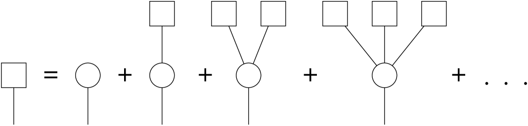
Figure 3: Schematic representation of the possible forms for the connected component of vertices reached by following a randomly chosen edge. The total probability of all possible forms (left-hand side) can be represented self-consistently as the sum of the probabilities (right-hand side) of having only a single vertex (the circle), having a single vertex connected to one other component, or two other components, and so forth. The entire sum can be expressed in closed form as Eq. (25).

Given this, we can calculate the distribution of component sizes below the transition as follows. Consider a randomly chosen edge somewhere in our graph and imagine following that edge to one of its ends and then to every other vertex reachable from that end. This set of vertices we refer to as the cluster at the end of a randomly chosen edge. Let $H_{1}(x)$ be the generating function that generates the distribution of sizes of such clusters, in terms of numbers of vertices. Each cluster can take many different forms, as shown in Fig. 3. We can follow our randomly chosen edge and find only a single vertex at its end, with no further edges emanating from it. Or we can find a vertex with one or more edges emanating from it. Each edge then leads to another complete cluster whose size is also distributed according to $H_{1}(x)$.

The number of edges $k$ emanating from our vertex, other than the one along which we arrived, is distributed according to the distribution $q_{k}$ of Eq. (4), and, using the multiplication property of generating functions from Section 3.1, the distribution of the sum of the sizes of the $k$ clusters that they lead to is generated by $[H_{1}(x)]^{k}$. Thus the total number of vertices reachable by following our randomly chosen edge is generated by

$$H_{1}(x)=x\sum_{k=0}^{\infty}q_{k}[H_{1}(x)]^{k}=xG_{1}(H_{1}(x)),$$ (25)

where the leading factor of $x$ accounts for the one vertex at the end of our edge, and we have made use of Eq. (14).

The quantity we actually want to know is the distribution of the sizes of the clusters to which a randomly chosen vertex belongs. The number of edges emanating from such a vertex is distributed according to the degree distribution $p_{k}$, and each such edge leads to a cluster whose size in vertices is drawn from the distribution generated by the function $H_{1}(x)$ above. Thus the size of the complete component to which a randomly vertex belongs is generated by

$$H_{0}(x)=x\sum_{k=0}^{\infty}p_{k}[H_{1}(x)]^{k}=xG_{0}(H_{1}(x)).$$ (26)

Now we can calculate the complete distribution of component sizes by solving (25) self-consistently for $H_{1}(x)$ and then substituting the result into (26).

Consider for instance the third example from Section 3.2, of a graph in which all vertices have degree three or less. Then Eq. (25) implies that $u=H_{1}(x)$ is a solution of the quadratic equation

$$q_{2}u^{2}+\left(q_{1}-{1\over x}\right)u+q_{0}=0,$$ (27)

or

$$H_{1}(x)={{1\over x}-q_{1}\pm\sqrt{\bigl{(}q_{1}-{1\over x}\bigr{)}^{2}-4q_{0}q_{2}}\over 2q_{2}}.$$ (28)

Substituting this into Eq. (26) and differentiating $m$ times then gives the probability that a randomly chosen vertex belongs to a component of exactly $m$ vertices total.

Unfortunately, cases such as this in which we can solve exactly for $H_{0}(x)$ and $H_{1}(x)$ are rare. More often no closed-form solution is possible. (For the simple Poissonian case of the Erdős–Rényi random graph, for instance, Eq. (25) is transcendental and has no closed-form solution.) We can still find closed-form expressions for the generating functions up to any finite order in $x$ however, by iteration of (25). To see this, suppose that we have an approximate expression for $H_{1}(x)$ that is correct up to some finite order $x^{m}$, but possibly incorrect at order $x^{m+1}$ and higher. If we substitute this approximate expression into the right-hand side of Eq. (25), we get a new expression for $H_{1}(x)$ and, because of the leading factor of $x$, the only contributions to the coefficient of $x^{m+1}$ in this expression come from the coefficients of $x^{m}$ and lower in the old expression. Since these lower coefficients were exactly correct, it immediately follows that the coefficient of $x^{m+1}$ in the new expression is correct also. Thus, if we start with the expression $H_{1}(x)=q_{0}x$, which is correct to order $x^{1}$, substitute it into (25), and iterate, then on each iteration we will generate an expression for $H_{1}(x)$ that is accurate to one order higher. After $m$ iterations, we will have an expression in which the coefficients for all orders up to and including $x^{m+1}$ are exactly correct.

Take for example the Erdős–Rényi random graph with its Poisson degree distribution, for which $G_{0}(x)=G_{1}(x)={\rm e}^{z(x-1)}$, as shown in Section 3.2. Then, noting that $q_{0}={\rm e}^{-z}$ for this case, we find that the first few iterations of Eq. (25) give

$$zH_{1}^{(1)}(x) = xz{\rm e}^{-z}+{\rm O}(x^{2}),$$ (29a)

$$zH_{1}^{(2)}(x) = xz{\rm e}^{-z}+(xz{\rm e}^{-z})^{2}+{\rm O}(x^{3}),$$

$$\vdots$$

$$zH_{1}^{(5)}(x) = xz{\rm e}^{-z}+(xz{\rm e}^{-z})^{2}+\mbox{$\frac{3}{2}$}(xz{\rm e}^{-z})^{3}+\mbox{$\frac{5}{3}$}(xz{\rm e}^{-z})^{4}+\mbox{$\frac{8}{3}$}(xz{\rm e}^{-z})^{5}+{\rm O}(x^{6}),$$

and so forth, from which we conclude that the probabilities $P_{s}$ of a randomly chosen site belonging to components of size $s=1,2,3\ldots$ are

$$P_{1}={\rm e}^{-z},\quad P_{2}=z{\rm e}^{-2z},\quad P_{3}=\mbox{$\frac{3}{2}$}z^{2}{\rm e}^{-3z},\quad P_{4}=\mbox{$\frac{5}{3}$}z^{3}{\rm e}^{-4z},\quad P_{5}=\mbox{$\frac{8}{3}$}z^{4}{\rm e}^{-5z}.$$ (30)

With a good symbolic manipulation program it is straightforward to calculate such probabilities to order 100 or so. If we require probabilities to higher order it is still possible to use Eqs. (25) and (26) to get answers, by iterating (25) numerically from a starting value of $H_{1}(x)=q_{0}x$. Doing this for a variety of different values of $x$ close to $x=0$, we can use the results to calculate the derivatives of $H_{0}(x)$ and so evaluate the $P_{s}$. Unfortunately, this technique is only usable for the first few $P_{s}$, because, as is usually the case with numerical derivatives, limits on the precision of floating-point numbers result in large errors at higher orders. To circumvent this problem we can employ a technique suggested by Moore and Newman (2000), and evaluate the derivatives instead by numerically integrating the Cauchy formula

$$P_{s}={1\over s!}{\partial^{s}H_{0}\over\partial x^{s}}\biggr{|}_{x=0}={1\over 2\pi{\rm i}}\oint{H_{0}(\zeta)\>{\rm d}\zeta\over\zeta^{s}},$$ (31)

where the integral is performed around any contour surrounding the origin but inside the first pole in $H_{0}(\zeta)$. For the best precision, Moore and Newman suggest using the largest such contour possible. In the present case, where $P_{s}$ is a properly normalized probability distribution, it is straightforward to show that $H_{0}(\zeta)$ must always converge within the unit circle and hence we recommend using this circle as the contour. Doing so appears to give excellent results in practice (Newman et al., 2001), with a thousand or more derivatives easily calculable in reasonable time.

4.2 Mean component size

Although, as we have seen, it is not usually possible to calculate the probability distribution of component sizes $P_{s}$ to all orders in closed form, we can calculate moments of the distribution, which in many cases is more useful anyway. The simplest case is the first moment, the mean component size. As we saw in Section 3.1, the mean of the distribution generated by a generating function is given by the derivative of the generating function evaluated at unity (Eq. (16)). Below the phase transition, the component size distribution is generated by $H_{0}(x)$, Eq. (26), and hence the mean component size below the transition is

$$\langle s\rangle=H_{0}^{\prime}(1)=\bigl{[}G_{0}(H_{1}(x))+xG_{0}^{\prime}(H_{1}(x))H_{1}^{\prime}(x)\bigr{]}_{x=1}=1+G_{0}^{\prime}(1)H_{1}^{\prime}(1),$$ (32)

where we have made use of the fact, Eq. (15), that properly normalized generating functions are equal to 1 at $x=1$, so that $G_{0}(1)=H_{1}(1)=1$. The value of $H_{1}^{\prime}(1)$ we can calculate from Eq. (25) by differentiating and rearranging to give

$$H_{1}^{\prime}(1)={1\over 1-G_{1}^{\prime}(1)},$$ (33)

and substituting into (32) we find

$$\langle s\rangle=1+{G_{0}^{\prime}(1)\over 1-G_{1}^{\prime}(1)}.$$ (34)

This expression can also be written in a number of other forms. For example, we note that

$$G_{0}^{\prime}(1) = \sum_{k}kp_{k}=\langle k\rangle=z_{1},$$ (35)

$$G_{1}^{\prime}(1) = {\sum_{k}k(k-1)p_{k}\over\sum_{k}kp_{k}}={\langle k^{2}\rangle-\langle k\rangle\over\langle k\rangle}={z_{2}\over z_{1}},$$ (36)

where we have made use of Eq. (6). Substituting into (34) then gives the average component size below the transition as

$$\langle s\rangle=1+{z_{1}^{2}\over z_{1}-z_{2}}.$$ (37)

This expression has a divergence at $z_{1}=z_{2}$, which signifies the formation of the giant component and gives an alternative and more rigorous derivation of the position of the critical point to that given in Section 2. Using Eq. (34), we could also write the condition for the phase transition as $G_{1}^{\prime}(1)=1$.

4.3 Above the phase transition

The calculations of the previous sections concerned the behaviour of the graph below the phase transition where there is no giant component in the graph. Almost all graphs studied empirically seem to be in the regime above the transition and do have a giant component. (This may be a tautologous statement, since it probably rarely occurs to researchers to consider a network representation of a set of objects or people so loosely linked that there is no connection between most pairs.) Can our generating function techniques be extended to this regime? As we now show, they can, although we will have to use some tricks to make things work. The problem is that the giant component is not a component like those we have considered so far. Those components had a finite average size, which meant that in the limit of large graph size they were all tree-like, containing no closed loops, as discussed in Section 4.1. The giant component, on the other hand, scales, by definition, as the size of the graph as a whole, and therefore becomes infinite as $n\to\infty$. This means that there will in general be loops in the giant component, which makes all the arguments of the previous sections break down. This problem can be fixed however by the following simple ploy. Above the transition, we define $H_{0}(x)$ and $H_{1}(x)$ to be the generating functions for the distributions of component sizes excluding the giant component. The non-giant components are still tree-like even above the transition, so Eqs. (25) and (26) are correct for this definition. The only difference is that now $H_{0}(1)$ is no longer equal to 1 (and neither is $H_{1}(1)$). Instead,

$$H_{0}(1)=\sum_{s}P_{s}=\mbox{fraction of vertices not in giant component},$$ (38)

which follows because the sum over $s$ is now over only the non-giant components, so the probabilities $P_{s}$ no longer add up to 1. This result is very useful; it allows us to calculate the size $S$ of the giant component above the transition as a fraction of the total graph size, since $S=1-H_{0}(1)$. From Eqs. (25) and (26), we can see that $S$ must be the solution of the equations

$$S=1-G_{0}(v),\qquad v=G_{1}(v),$$ (39)

where $v\equiv H_{1}(1)$. As with the calculation of the component size distribution in Section 4.1, these equations are not normally solvable in closed form, but a solution can be found to arbitrary numerical accuracy by iteration starting from a suitable initial value of $v$, such as $v=0$.

We can also calculate the average sizes of the non-giant components in the standard way by differentiating Eq. (26). We must be careful however, for a couple of reasons. First, we can no longer assume that $H_{0}(1)=H_{1}(1)=1$ as is the case below the transition. Second, since the distribution $P_{s}$ is not normalized to 1, we have to perform the normalization ourselves. The correct expression for the average component size is

$$\langle s\rangle = {H_{0}^{\prime}(1)\over H_{0}(1)}={1\over H_{0}(1)}\biggl{[}G_{0}(H_{1}(1))+{G_{0}^{\prime}(H_{1}(1))G_{1}(H_{1}(1))\over 1-G_{1}^{\prime}(H_{1}(1))}\biggr{]}$$ (40)

$$= 1+{zv^{2}\over[1-S][1-G_{1}^{\prime}(v)]},$$

where $v$ and $S$ are found from Eq. (39). It is straightforward to verify that this becomes equal to Eq. (34) when we are below the transition and $S=0$, $v=1$.

Figure 4: Behaviour of a random graph with an exponential degree distribution of the form of Eq. (20). Top: fraction of the graph occupied by the giant component. Bottom: average component size. Note that the horizontal axis is logarithmic.

As an example of these results, we show in Fig. 4 the size of the giant component and the average (non-giant) component size for graphs with an exponential degree distribution of the form of Eq. (20), as a function of the exponential constant $\kappa$. As the figure shows, there is a divergence in the average component size at the phase transition, with the giant component becoming non-zero smoothly above the transition. Those accustomed to the physics of continuous phase transitions will find this behaviour familiar; the size of the giant component acts as an order parameter here, as it did in the Erdős–Rényi random graph in the introduction to this paper, and the average component size behaves like a susceptibility. Indeed one can define and calculate critical exponents for the transition using this analogy, and as with the Erdős–Rényi model, their values put us in the same universality class as the mean-field (i.e., infinite dimension) percolation transition (Newman et al., 2001). The phase transition in Fig. 4 takes place just a little below $\kappa=1$ when $G_{1}^{\prime}(1)=1$, which gives a critical value of $\kappa_{c}=(\log 3)^{-1}=0.910\ldots$

5 Properties of directed graphs

Some of the graphs discussed in the introduction to this paper are directed graphs. That is, the edges in the network have a direction to them. Examples are the World-Wide Web, in which hyperlinks from one page to another point in only one direction, and food webs, in which predator–prey interactions are asymmetric and can be thought of as pointing from predator to prey. Other recently studied examples of directed networks include telephone call graphs (Abello et al., 1998; Hayes, 2000; Aiello et al., 2000), citation networks (Redner, 1998; Vazquez, 2001), and email networks (Ebel et al., 2002).

Directed networks are more complex than their undirected counterparts. For a start, each vertex in an directed network has two degrees, an in-degree, which is the number of edges that point into the vertex, and an out-degree, which is the number pointing out. There are also, correspondingly, two degree distributions. In fact, to be completely general, we must allow for a joint degree distribution of in- and out-degree: we define $p_{jk}$ to be the probability that a randomly chosen vertex simultaneously has in-degree $j$ and out-degree $k$. Defining a joint distribution like this allows for the possibility that the in- and out-degrees may be correlated. For example in a graph where every vertex had precisely the same in- and out-degree, $p_{jk}$ would be non-zero if and only if $j=k$.

The component structure of a directed graph is more complex than that of an undirected graph also, because a directed path may exist through the network from vertex A to vertex B, but that does not guarantee that one exists from B to A. As a result, any vertex A belongs to components of four different types:

1. The in-component is the set of vertices from which A can be reached.

2. The out-component is the set of vertices which can be reached from A.

3. The strongly connected component is the set of vertices from which vertex A can be reached and which can be reached from A.

4. The weakly connected component is the set of vertices that can be reached from A ignoring the directed nature of the edges altogether.

The weakly connected component is just the normal component to which A belongs if one treats the graph as undirected. Clearly the details of weakly connected components can be worked out using the formalism of Section 4, so we will ignore this case. For vertex A to belong to a strongly connected component of size greater than one, there must be at least one other vertex that can both be reached from A and from which A can be reached. This however implies that there is a closed loop of directed edges in the graph, something which, as we saw in Section 4.1, does not happen in the limit of large graph size. So we ignore this case also. The two remaining cases, the in- and out-components, we consider in more detail in the following sections.

5.1 Generating functions

Because the degree distribution $p_{jk}$ for a directed graph is a function of two variables, the corresponding generating function is also:

$$\mathcal{G}(x,y)=\sum_{j,k=0}^{\infty}p_{jk}x^{j}y^{k}.$$ (41)

This function satisfies the normalization condition $\mathcal{G}(1,1)=1$, and the means of the in- and out-degree distributions are given by its first derivatives with respect to $x$ and $y$. However, there is only one mean degree $z$ for a directed graph, since every edge must start and end at a site. This means that the total and hence also the average numbers of in-going and out-going edges are the same. This gives rise to a constraint on the generating function of the form

$${\partial\mathcal{G}\over\partial x}\bigg{|}_{x,y=1}=z={\partial\mathcal{G}\over\partial y}\bigg{|}_{x,y=1},$$ (42)

and there is a corresponding constraint on the probability distribution $p_{jk}$ itself, which can be written

$$\sum_{jk}(j-k)p_{jk}=0.$$ (43)

From $\mathcal{G}(x,y)$, we can now define single-argument generating functions $G_{0}$ and $G_{1}$ for the number of out-going edges leaving a randomly chosen vertex, and the number leaving the vertex reached by following a randomly chosen edge. These play a similar role to the functions of the same name in Section 4. We can also define generating functions $F_{0}$ and $F_{1}$ for the number of edges arriving at a vertex. These functions are given by

$$F_{0}(x) = \mathcal{G}(x,1),\qquad F_{1}(x)={1\over z}\,{\partial\mathcal{G}\over\partial y}\bigg{|}_{y=1},$$ (44)

$$G_{0}(y) = \mathcal{G}(1,y),\hskip 21.33955ptG_{1}(y)={1\over z}\,{\partial\mathcal{G}\over\partial x}\bigg{|}_{x=1}.$$ (45)

Once we have these functions, many results follow as before.

5.2 Results

The probability distribution of the numbers of vertices reachable from a randomly chosen vertex in a directed graph—i.e., of the sizes of the out-components—is generated by the function $H_{0}(y)=yG_{0}(H_{1}(y))$, where $H_{1}(y)$ is a solution of $H_{1}(y)=yG_{1}(H_{1}(y))$, just as before. (A similar and obvious pair of equations governs the sizes of the in-components.) The average out-component size for the case where there is no giant component is then given by Eq. (34), and thus the point at which a giant component first appears is given once more by $G_{1}^{\prime}(1)=1$. Substituting Eq. (45) into this expression gives the explicit condition

$$\sum_{jk}(2jk-j-k)p_{jk}=0$$ (46)

for the first appearance of the giant component. This expression is the equivalent for the directed graph of Eq. (9). It is also possible, and equally valid, to define the position at which the giant component appears by $F_{1}^{\prime}(1)=1$, which provides an alternative derivation for Eq. (46).

But this raises an interesting issue. Which giant component are we talking about? Just as with the small components, there are four types of giant component, the giant in- and out-components, and the giant weakly and strongly connected components. Furthermore, while the giant weakly connected component is as before trivial, the giant strongly connected component does not normally vanish as the other strongly connected components do. There is no reason why a giant component should contain no loops, and therefore no reason why we should not have a non-zero giant strongly connected component.

The condition for the position of the phase transition given above is derived from the point at which the mean size of the out-component reachable from a vertex diverges, and thus this is the position at which the giant in-component forms (since above this point an extensive number of vertices can be reached starting from one vertex, and hence that vertex must belong to the giant in-component). Furthermore, as we have seen, we get the same condition if we ask where the mean in-component size diverges, i.e., where the giant out-component forms, and so we conclude that both giant in- and out-components appear at the same time, at the point given by Eq. (46).

The sizes of these two giant components can also be calculated with only a little extra effort. As before, we can generalize the functions $H_{0}(y)$ and $H_{1}(y)$ to the regime above the transition by defining them to be the generating functions for the non-giant out-components in this regime. In that case, $H_{0}(1)$ is equal to the fraction of all vertices that have a finite out-component. But any vertex A that has only a finite out-component cannot, by definition, belong to the giant in-component, i.e., there definitely do not exist an extensive number of vertices that can be reached from A. Thus the size of the giant in-component is simply $S_{\rm in}=1-H_{0}(1)$, which can be calculated as before from Eq. (39). Similarly the size of the giant out-component can be calculated from (39) with $G_{0}\to F_{0}$ and $G_{1}\to F_{1}$.

To calculate the size of the giant strongly connected component, we observe the following (Dorogovtsev et al., 2001). If at least one of a vertex’s outgoing edges leads to anywhere in the giant in-component, then one can reach the giant strongly connected component from that vertex. Conversely, if at least one of a vertex’s incoming edges leads from anywhere in the giant out-component, then the vertex can be reached from the strongly connected component. If and only if both of these conditions are satisfied simultaneously, then the vertex belongs to the giant strongly connected component itself.

Consider then the outgoing edges. The function $H_{1}(x)$ gives the probability distribution of the sizes of finite out-components reached by following a randomly chosen edge. This implies that $H_{1}(1)$ is the total probability that an edge leads to a finite out-component (i.e., not to the giant in-component) and as before (Eq. (39)) $H_{1}(1)$ is the fixed point of $G_{1}(x)$, which we denote by $v$. For a vertex with $k$ outgoing edges, $v^{k}$ is then the probability that all of them lead to finite components and $1-v^{k}$ is the probability that at least one edge leads to the giant in-component. Similarly the probability that at least one incoming edge leads from the giant out-component is $1-u^{j}$, where $u$ is the fixed point of $F_{1}(x)$ and $j$ is the in-degree of the vertex. Thus the probability that a vertex with in- and out-degrees $j$ and $k$ is in the giant strongly connected component is $(1-u^{j})(1-v^{k})$, and the average of this probability over all vertices, which is also the fractional size of the giant strongly connected component, is

$$S_{s} = \sum_{jk}p_{jk}(1-u^{j})(1-v^{k})=\sum_{jk}p_{jk}(1-u^{j}-v^{k}+u^{j}v^{k})$$ (47)

$$= 1-\mathcal{G}(u,1)-\mathcal{G}(1,v)+\mathcal{G}(u,v),$$

where $u$ and $v$ are solutions of

$$u=F_{1}(u),\qquad v=G_{1}(v),$$ (48)

and we have made use of the definition, Eq. (41), of $\mathcal{G}(x,y)$. Noting that $u=v=1$ below the transition at which the giant in- and out-components appear, and that $\mathcal{G}(1,1)=1$, we see that the giant strongly connected component also first appears at the transition point given by Eq. (46). Thus there are in general two phase transitions in a directed graph: the one at which the giant weakly connected component appears, and the one at which the other three giant components all appear.

Applying the theory of directed random graphs to real directed networks has proved difficult so far, because experimenters rarely measure the joint in- and out-degree distribution $p_{jk}$ that is needed to perform the calculations described above. A few results can be calculated without the joint distribution—see Newman et al. (2001), for instance. By and large, however, the theory presented in this section is still awaiting empirical tests.

6 Networks with clustering

Far fewer analytical results exist for networks that incorporate clustering than for the non-clustered networks of the previous sections. A first attempt at extending random graph models to incorporate clustering has been made by the present author, who studied the correction to the quantity $z_{2}$—the average number of next-nearest neighbours of a vertex—in graphs with a non-zero clustering coefficient $C$ (Newman, 2001d).

Consider a vertex A, with its first and second neighbours in the network arrayed around it in two concentric rings. In a normal random graph, a neighbour of A that has degree $m$ contributes $m-1$ vertices to the ring of second neighbours of A, as discussed in Section 2. That is, all of the second neighbours of A are independent; each of them is a new vertex never before seen. This is the reasoning that led to our earlier expression, Eq. (6): $z_{2}=\langle k^{2}\rangle-\langle k\rangle$. In a clustered network however, the picture is different. In a clustered network, many of the neighbours of A’s neighbour are neighbours of A themselves. This is the meaning of clustering: your friend’s friend is also your friend. In fact, by definition, an average fraction $C$ of the $m-1$ neighbours are themselves neighbours of the central vertex A and hence should not be counted as second neighbours. Correspondingly, this reduces our estimate of $z_{2}$ by a factor of $1-C$ to give $z_{2}=(1-C)(\langle k^{2}\rangle-\langle k\rangle)$.

But this is not all. There is another effect we need to take into account if we are to estimate $z_{2}$ correctly. It is also possible that we are overcounting the second neighbours of A because some of them are neighbours of more than one of the first neighbours. In other words, you may know two people who have another friend in common, whom you personally don’t know. Such connections create “squares” in the network, whose density can be quantified by the so-called mutuality $M$:

$$M={\mbox{mean number of vertices two steps away from a vertex}\over\mbox{mean number of paths of length two to those vertices}}.$$ (49)

In words, $M$ measures the average number of paths of length two leading to a vertex’s second neighbour. As a result of the mutuality effect, our current estimate of $z_{2}$ will be too great by a factor of $1/M$, and hence a better estimate is

$$z_{2}=M(1-C)(\langle k^{2}\rangle-\langle k\rangle).$$ (50)

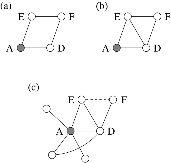
Figure 5: (a) An example of a vertex (F) that is two steps away from the center vertex (A, shaded), but is connected to two of A’s neighbours (D and E). F should only be counted once as a second neighbour of A, not twice. (b) A similar situation in which D and E are also neighbours of one another. (c) The probability of situation (b) can be calculated by considering this situation. Since D is friends with both E and F, the probability that E and F also know one another (dotted line), thereby completing the quadrilateral in (b), is by definition equal to the clustering coefficient.

But now we have a problem. Calculating the mutuality $M$ using Eq. (49) requires that we know the mean number of individuals two steps away from the central vertex A. But this mean number is precisely the quantity $z_{2}$ that our calculation is supposed to estimate in the first place. There is a partial solution to this problem. Consider the two configurations depicted in Fig. 5, parts (a) and (b). In (a) our vertex A has two neighbours D and E, both of whom are connected to F, although F is not itself an neighbour of A. The same is true in (b), but now D and E are friends of one another also. Empirically, it appears that in many networks situation (a) is quite uncommon, while situation (b) is much more common. And we can estimate the frequency of occurrence of (b) from a knowledge of the clustering coefficient.

Consider Fig. 5c. The central vertex A shares an edge with D, which shares an edge with F. How many other paths of length two are there from A to F? Well, if A has $k_{1}$ neighbours, then by the definition of the clustering coefficient, D will be connected to $C(k_{1}-1)$ of them on average. The edge between vertices D and E in the figure is an example of one such. But now D is connected to both E and F, and hence, using the definition of the clustering coefficient again, E and F will themselves be connected (dotted line) with probability equal to the clustering coefficient $C$. Thus there will on average be $C^{2}(k_{1}-1)$ other paths of length 2 to F, or $1+C^{2}(k_{1}-1)$ paths in total, counting the one that runs through D. This is the average factor by which we will overcount the number of second neighbours of A because of the mutuality effect. As shown by Newman (2001d), the mutuality coefficient is then given by

$$M={\langle k/[1+C^{2}(k-1)]\rangle\over\langle k\rangle}.$$ (51)

Substituting this into Eq. (50) then gives us an estimate of $z_{2}$.

In essence what Eq. (51) does is estimate the value of $M$ in a network in which triangles of ties are common, but squares that are not composed of adjacent triangles are assumed to occur with frequency no greater than one would expect in a purely random network. It is only an approximate expression, since this assumption will usually not be obeyed perfectly. Nonetheless, it appears to give good results. The author applied Eqs. (50) and (51) to estimation of $z_{2}$ for the two coauthorship networks of Fig. 1c, and found that they gave results accurate to within 10% in both cases.

This calculation is certainly only a first step. Ideally we would like to be able to calculate numbers of vertices at any distance from a randomly chosen central vertex in the presence of clustering, and to do it exactly rather than just approximately. If this were possible, then, as in Section 2, one could use the ratio of the numbers of vertices at different distances to derive a condition for the position of the phase transition at which a giant component forms on a clustered graph. At present it is not clear if such a calculation is possible.

7 Models defined on random graphs

In addition to providing an analytic framework for calculating topological properties of networks, such as typical path lengths or distributions of cluster sizes, random graphs form a useful substrate for studying the behaviour of phenomena that take place on networks. Analytic work in this area is in its infancy; here we describe two examples of recent work on models that use ideas drawn from percolation theory.

7.1 Network resilience

As emphasized by Albert and co-workers, the highly skewed degree distributions of Fig. 1 have substantial implications for the robustness of networks to the removal of vertices (Albert et al., 2000). Because most of the vertices in a network with such a degree distribution typically have low degree, the random removal of vertices from the network has little effect on the connectivity of the remaining vertices, i.e., on the existence of paths between pairs of vertices, a crucial property of networks such as the Internet, for which functionality relies on connectivity. In particular, removal of vertices with degree zero or one will never have any effect on the connectivity of the remaining vertices. (Vertices of degree zero are not connected to anyone else anyway, and vertices of degree one do not lie on any path between another pair of vertices.)

Conversely, however, the specific removal of the vertices in the network with the highest degree frequently has a devastating effect. These vertices lie on many of the paths between pairs of other vertices and their removal can destroy the connectivity of the network in short order. This was first demonstrated numerically by Albert et al. (2000) and independently by Broder et al. (2000) using data for subsets of the World-Wide Web. More recently however it has been demonstrated analytically also, for random graphs with arbitrary degree distributions, by Callaway et al. (2000) and by Cohen et al. (2001). Here we follow the derivation of Callaway et al., which closely mirrors some of the earlier mathematical developments of this paper.

Consider a simple model defined on a network in which each vertex is either “present” or “absent”. Absent vertices are vertices that have either been removed, or more realistically are present but non-functional, such as Internet routers that have failed or Web sites whose host computer has gone down. We define a probability $b_{k}$ of being present which is some arbitrary function of the degree $k$ of a vertex, and then define the generating function

$$F_{0}(x)=\sum_{k=0}^{\infty}p_{k}b_{k}x^{k},$$ (52)

whose coefficients are the probabilities that a vertex has degree $k$ and is present. Note that this generating function is not equal to 1 at $x=1$; instead it is equal to the fraction of all vertices that are present. By analogy with Eq. (14) we also define

$$F_{1}(x)=\frac{\sum_{k}kp_{k}b_{k}x^{k-1}}{\sum_{k}kp_{k}}=\frac{F_{0}^{\prime}(x)}{z}.$$ (53)

Then the distributions of the sizes of connected clusters of present vertices reachable from a randomly chosen vertex or edge are generated respectively by

$$H_{0}(x)=1-F_{0}(1)+xF_{0}(H_{1}(x)),\qquad H_{1}(x)=1-F_{1}(1)+xF_{1}(H_{1}(x)),$$ (54)

which are logical equivalents of Eqs. (25) and (26).

Take for instance the case of random failure of vertices. In this case, the probability $b_{k}$ of a vertex being present is independent of the degree $k$ and just equal to a constant $b$, which means that

$$H_{0}(x)=1-b+bxG_{0}(H_{1}(x)),\qquad H_{1}(x)=1-b+bxG_{1}(H_{1}(x)),$$ (55)

where $G_{0}(x)$ and $G_{1}(x)$ are the standard generating functions for vertex degree, Eqs. (12) and (14). This implies that the mean size of a cluster of connected and present vertices is

$$\langle s\rangle=H_{0}^{\prime}(1)=b+bF_{0}^{\prime}(1)H_{1}^{\prime}(1)=b\left[1+\frac{bG_{0}^{\prime}(1)}{1-bG_{1}^{\prime}(1)}\right],$$ (56)

and the model has a phase transition at the critical value of $b$

$$b_{c}=\frac{1}{G_{1}^{\prime}(1)}.$$ (57)

If a fraction $b<b_{c}$ of the vertices are present in the network, then there will be no giant component. This is the point at which the network ceases to be functional in terms of connectivity. When there is no giant component, connecting paths exist only within small isolated groups of vertices, but no long-range connectivity exists. For a communication network such as the Internet, this would be fatal. As we would expect from the arguments above however, $b_{c}$ is usually a very small number for networks with skewed degree distributions. For example, if a network has a pure power-law degree distribution with exponent $\alpha$, as both the Internet and the World-Wide Web appear to do (see Fig. 1a and 1b), then

$$b_{c}={\zeta(\alpha-1)\over\zeta(\alpha-2)-\zeta(\alpha-1)},$$ (58)

where $\zeta(x)$ is the Riemann $\zeta$-function. This expression is formally zero for all $\alpha\leq 3$. Since none of the distributions in Fig. 1 have an exponent greater than 3, it follows that, at least to the extent that these graphs can be modelled as random graphs, none of them has a phase transition at all. No matter how many vertices fail in these networks, as long as the failing vertices are selected at random without regard for degree, there will always be a giant component in the network and an extensive fraction of the vertices will be connected to one another. In this sense, networks with power-law distributed degrees are highly robust, as the numerical experiments of Albert et al. (2000) and Broder et al. (2000) also found.

But now consider the case in which the vertices are removed in decreasing order of their degrees, starting with the highest degree vertex. Mathematically we can represent this by setting

$$b_{k}=\theta(k_{\rm max}-k),$$ (59)

where $\theta(x)$ is the Heaviside step function

$$\theta(x)=\biggl{\{}\begin{array}[]{ll}0&\mbox{for $x<0$}\\ 1\hbox{}&\mbox{for $x\geq 0$.}\end{array}$$ (60)

This is equivalent to setting the upper limit of the sum in Eq. (52) to $k_{\rm max}$.

For this case we need to use the full definition of $H_{0}(x)$ and $H_{1}(x)$, Eq. (54), which gives the position of the phase transition as the point at which $F_{1}^{\prime}(1)=1$, or

$${\sum_{k=1}^{\infty}k(k-1)p_{k}b_{k}\over\sum_{k=1}^{\infty}kp_{k}}=1.$$ (61)

Taking the example of our power-law degree distribution again, $p_{k}\propto k^{-\alpha}$, this then implies that the phase transition occurs at a value $k_{c}$ of $k_{\rm max}$ satisfying

$$H_{k_{c}}^{(\alpha-2)}-H_{k_{c}}^{(\alpha-1)}=\zeta(\alpha-1),$$ (62)

where $H_{n}^{(r)}$ is the $n$th harmonic number of order $r$:

$$H_{n}^{(r)}=\sum_{k=1}^{n}{1\over k^{r}}.$$ (63)

This solution is not in a very useful form however. What we really want to know is what fraction $f_{c}$ of the vertices have been removed when we reach the transition. This fraction is given by

$$f_{c}=1-{H_{k_{c}}^{(\alpha)}\over\zeta(\alpha)}.$$ (64)

Although we cannot eliminate $k_{c}$ from (62) and (64) to get $f_{c}$ in closed form, we can solve Eq. (62) numerically for $k_{c}$ and substitute into (64). The result is shown as a function of $\alpha$ in Fig. 6. As the figure shows, one need only remove a very small fraction of the high-degree vertices to destroy the giant component in a power-law graph, always less than 3%, with the most robust graphs being those around $\alpha=2.2$, interestingly quite close to the exponent seen in a number of real-world networks (Fig. (1)). Below $\alpha=2$, there is no real solution for $f_{c}$: power-law distributions with $\alpha<2$ have no finite mean anyway and therefore make little sense physically. And $f_{c}=0$ for all values $\alpha>3.4788\ldots$, where the latter figure is the solution of $\zeta(\alpha-2)=2\zeta(\alpha-1)$, because the underlying network itself has no giant component for such values of $\alpha$ (Aiello et al., 2000).

Figure 6: The critical fraction, Eq. (64), of highest degree vertices that must be removed in order to destroy the giant component in a graph with a power-law degree distribution having exponent $\alpha$.

Overall, therefore, our results agree with the findings of the previous numerical studies that graphs with skewed degree distributions, such as power laws, can be highly robust to the random removal of vertices, but extremely fragile to the specific removal of their highest-degree vertices.

7.2 Epidemiology

An important application of the theory of networks is in epidemiology, the study of the spread of disease. Diseases are communicated from one host to another by physical contact, and the pattern of who has contact with whom forms a contact network whose structure has implications for the shape of epidemics. In particular, the small-world effect discussed in Section 2 means that diseases will spread through a community much faster than one might otherwise imagine.

In the standard mathematical treatments of diseases, researchers use the so-called fully mixed approximation, in which it is assumed that every individual has equal chance of contact with every other. This is an unrealistic assumption, but it has proven popular because it allows one to write differential equations for the time evolution of the disease that can be solved or numerically integrated with relative ease. More realistic treatments have also been given in which populations are divided into groups according to age or other characteristics. These models are still fully mixed within each group however. To go beyond these approximations, we need to incorporate a full network structure into the model, and the random graphs of this paper and the generating function methods we have developed to handle them provide a good basis for doing this.

In this section we show that the most fundamental standard model of disease propagation, the SIR model, and a large set of its generalized forms, can be solved on random graphs by mapping them onto percolation problems. These solutions provide exact criteria for deciding when an epidemic will occur, how many people will be affected, and how the network structure or the transmission properties of the disease could be modified in order to prevent the epidemic.

7.3 The SIR model

First formulated (though never published) by Lowell Reed and Wade Hampton Frost in the 1920s, the SIR model (Bailey, 1975; Anderson and May, 1991; Hethcote, 2000) is a model of disease propagation in which members of a population are divided into three classes: susceptible (S), meaning they are free of the disease but can catch it; infective (I), meaning they have the disease and can pass it on to others; and removed (R), meaning they have recovered from the disease or died, and can no longer pass it on. There is a fixed probability per unit time that an infective individual will pass the disease to a susceptible individual with whom they have contact, rendering that individual infective. Individuals who contract the disease remain infective for a certain time period before recovering (or dying) and thereby losing their infectivity.

As first pointed out by Grassberger (1983), the SIR model on a network can be simply mapped to a bond percolation process. Consider an outbreak on a network that starts with a single individual and spreads to encompass some subset of the network. The vertices of the network represent potential hosts and the edges represent pairs of hosts who have contact with one another. If we imagine occupying or colouring in all the edges that result in transmission of the disease during the current outbreak, then the set of vertices representing the hosts infected in this outbreak form a connected percolation cluster of occupied edges. Furthermore, it is easy to convince oneself that each edge is occupied with independent probability. If we denote by $\tau$ the time for which an infected host remains infective and by $r$ the probability per unit time that that host will infect one of its neighbours in the network, then the total probability of infection is

$$T=1-\lim_{\delta t\to 0}(1-r\,\delta t)^{\tau/\delta t}=1-{\rm e}^{-r\tau}.$$ (65)

This quantity we call the transmissibility, and it is the probability that any edge on the network is occupied. The size distribution of outbreaks of the disease is then given by the size distribution of percolation clusters on the network when edges are occupied with this probability. When the mean cluster size diverges, we get outbreaks that occupy a finite fraction of the entire network, i.e., epidemics; the percolation threshold corresponds to what an epidemiologist would call the epidemic threshold for the disease. Above this threshold, there exists a giant component for the percolation problem, whose size corresponds to the size of the epidemic. Thus, if we can solve bond percolation on our random graphs, we can also solve the SIR model.

In fact, we can also solve a generalized form of the SIR in which both $\tau$ and $r$ are allowed to vary across the network. If $\tau$ and $r$ instead of being constant are picked at random for each vertex or edge from some distributions $P(\tau)$ and $P(r)$, then the probability of percolation along any edge is simply the average of Eq. (65) over these two distributions (Warren et al., 2001, 2002):

$$T=1-\int P(r)P(\tau)\,{\rm e}^{-r\tau}\>{\rm d}r\>{\rm d}\tau.$$ (66)

7.4 Solution of the SIR model

The bond percolation problem on a random graph can be solved by techniques very similar to those of Section 7.1 (Callaway et al., 2000; Newman, 2002). The equivalent of Eq. (55) for bond percolation with bond occupation probability $T$ is

$$H_{0}(x)=xG_{0}(H_{1}(x)),\qquad H_{1}(x)=1-T+TxG_{1}(H_{1}(x)),$$ (67)

which gives an average outbreak size below the epidemic threshold of

$$\langle s\rangle=H_{0}^{\prime}(1)=1+{TG_{0}^{\prime}(1)\over 1-TG_{1}^{\prime}(1)}.$$ (68)

The threshold itself then falls at the point where $TG_{1}^{\prime}(1)=1$, giving a critical transmissibility of

$$T_{c}={1\over G_{1}^{\prime}(1)}={\langle k\rangle\over\langle k^{2}\rangle-\langle k\rangle}={z_{1}\over z_{2}},$$ (69)

where we have used Eq. (6). The size $S$ of the epidemic above the epidemic transition can be calculated by finding the solution of

$$S=1-G_{0}(v),\qquad v=1-T+TG_{1}(v),$$ (70)

which will normally have to be solved numerically, since closed form solutions are rare. It is also interesting to ask what the probability is that an outbreak starting with a single carrier will become an epidemic. This is precisely equal to the probability that the carrier belongs to the giant percolating cluster, which is also just equal to $S$. The probability that a given infection event (i.e., transmission along a given edge) will give rise to an epidemic is $v\equiv H_{1}^{\prime}(1)$.

Newman and co-workers have given a variety of further generalizations of these solutions to networks with structure of various kinds, models in which the probabilities of transmission between pairs of hosts are correlated in various ways, and models incorporating vaccination, either random or targeted, which is represented as a site percolation process (Ancel et al., 2001; Newman, 2002). To give one example, consider the network by which a sexually transmitted disease is communicated, which is also the network of sexual partnerships between individuals. In a recent study of 2810 respondents, Liljeros et al. (2001) recorded the numbers of sexual partners of men and women over the course of a year. From their data it appears that the distributions of these numbers follow a power law similar to those of the distributions in Fig. 1, with exponents $\alpha$ that fall in the range $3.1$ to $3.3$. If we assume that the disease of interest is transmitted primarily by contacts between men and women (true only for some diseases), then to a good approximation the network of contacts is bipartite, having two separate sets of vertices representing men and women and edges representing contacts running only between vertices of unlike kinds. We define two pairs of generating functions for males and females:

$$F_{0}(x) = \sum_{j}p_{j}x^{j},\qquad F_{1}(x)=\frac{1}{\mu}\sum_{j}jp_{j}x^{j-1},$$ (71)

$$G_{0}(x) = \sum_{k}q_{k}x^{k},\hskip 19.34787ptG_{1}(x)=\frac{1}{\nu}\sum_{k}kq_{k}x^{k-1},$$ (72)

where $p_{j}$ and $q_{k}$ are the two degree distributions and $\mu$ and $\nu$ are their means. We can then develop expressions similar to Eqs. (68) and (69) for an epidemic on this new network. We find, for instance, that the epidemic transition takes place at the point where $T_{mf}T_{fm}=1/[F_{1}^{\prime}(1)G_{1}^{\prime}(1)]$ where $T_{mf}$ and $T_{fm}$ are the transmissibilities for male-to-female and female-to-male infection respectively.

One important result that follows immediately is that if the degree distributions are truly power-law in form, then there exists an epidemic transition only for a small range of values of the exponent $\alpha$ of the power law. Let us assume, as appears to be the case (Liljeros et al., 2001), that the exponents are roughly equal for men and women: $\alpha_{m}=\alpha_{f}=\alpha$. Then if $\alpha\leq 3$, we find that $T_{mf}T_{fm}=0$, which is only possible if at least one of the transmissibilities $T_{mf}$ and $T_{fm}$ is zero. As long as both are positive, we will always be in the epidemic regime, and this would clearly be bad news. No amount of precautionary measures to reduce the probability of transmission would ever eradicate the disease. (Similar results have been seen in other types of models also (Pastor-Satorras and Vespignani, 2001; Lloyd and May, 2001).) Conversely, if $\alpha>\alpha_{c}$, where $\alpha_{c}=3.4788\ldots$ is the solution of $\zeta(\alpha-2)=2\zeta(\alpha-1)$, we find that $T_{mf}T_{fm}>1$, which is not possible. (This latter result arises because networks with $\alpha>\alpha_{c}$ have no giant component at all, as mentioned in Section 7.1 (Aiello et al., 2000).) In this regime then, no epidemic can ever occur, which would be good news. Only in the small intermediate region $3<\alpha<3.4788\ldots$ does the model possess an epidemic transition. Interestingly, the real-world network measured by Liljeros et al. (2001) appears to fall precisely in this region, with $\alpha\simeq 3.2$. If true, this would be both good and bad news. On the bad side, it means that epidemics can occur. But on the good side, it means that that it is in theory possible to prevent an epidemic by reducing the probability of transmission, which is precisely what most health education campaigns attempt to do. The predicted critical value of the transmissibility is $\zeta(\alpha-1)/[\zeta(\alpha-2)-\zeta(\alpha-1)]$, which gives $T_{c}=0.363\ldots$ for $\alpha=3.2$. Epidemic behaviour would cease were it possible to arrange that $T_{mf}T_{fm}<T_{c}^{2}$.

8 Summary

In this paper we have given an introduction to the use of random graphs as models of real-world networks. We have shown (Section 2) how the much studied random graph model of Erdős and Rényi can be generalized to the case of arbitrary degree distributions, allowing us to mimic the highly skewed degree distributions seen in many networks. The resulting models can be solved exactly using generating function methods in the case where there is no clustering (Sections 3 and 4). If clustering is introduced, then solutions become significantly harder, and only a few approximate analytic results are known (Section 6). We have also given solutions for the properties of directed random graphs (Section 5), in which each edge has a direction that it points in. Directed graphs are useful as models of the World-Wide Web and food webs, amongst other things. In the last part of this paper (Section 7) we have given two examples of the use of random graphs as a substrate for models of dynamical processes taking place on networks, the first being a model of network robustness under failure of vertices (e.g., failure of routers on the Internet), and the second being a model of the spread of disease across the network of physical contacts between disease hosts. Both of these models can be mapped onto percolation problems of one kind of another, which can then be solved exactly, again using generating function methods.

There are many conceivable extensions of the theory presented in this paper. In particular, there is room for many more and diverse models of processes taking place on networks. It would also be of great interest if it proved possible to extend the results of Section 6 to obtain exact or approximate estimates of the global properties of networks with non-zero clustering.

- (1)
- Abello et al. (1998) Abello, J., Buchsbaum, A. and Westbrook, J., 1998. A functional approach to external graph algorithms. In Proceedings of the 6th European Symposium on Algorithms. Springer, Berlin.
- Adamic (1999) Adamic, L. A., 1999. The small world web. In Lecture Notes in Computer Science, volume 1696, pp. 443–454. Springer, New York.
- Aiello et al. (2000) Aiello, W., Chung, F. and Lu, L., 2000. A random graph model for massive graphs. In Proceedings of the 32nd Annual ACM Symposium on Theory of Computing, pp. 171–180. Association of Computing Machinery, New York.
- Albert and Barabási (2002) Albert, R. and Barabási, A.-L., 2002. Statistical mechanics of complex networks. Rev. Mod. Phys. 74, 47–97.
- Albert et al. (1999) Albert, R., Jeong, H. and Barabási, A.-L., 1999. Diameter of the world-wide web. Nature 401, 130–131.
- Albert et al. (2000) Albert, R., Jeong, H. and Barabási, A.-L., 2000. Attack and error tolerance of complex networks. Nature 406, 378–382.
- Amaral et al. (2000) Amaral, L. A. N., Scala, A., Barthélémy, M. and Stanley, H. E., 2000. Classes of small-world networks. Proc. Natl. Acad. Sci. USA 97, 11149–11152.
- Ancel et al. (2001) Ancel, L. W., Newman, M. E. J., Martin, M. and Schrag, S., 2001. Applying network theory to epidemics: Modelling the spread and control of Mycoplasma pneumoniae. Working paper 01–12–078, Santa Fe Institute.
- Anderson and May (1991) Anderson, R. M. and May, R. M., 1991. Infectious Diseases of Humans. Oxford University Press, Oxford.
- Bailey (1975) Bailey, N. T. J., 1975. The Mathematical Theory of Infectious Diseases and its Applications. Hafner Press, New York.
- Barabási and Albert (1999) Barabási, A.-L. and Albert, R., 1999. Emergence of scaling in random networks. Science 286, 509–512.
- Bender and Canfield (1978) Bender, E. A. and Canfield, E. R., 1978. The asymptotic number of labeled graphs with given degree sequences. Journal of Combinatorial Theory A 24, 296–307.
- Bollobás (1985) Bollobás, B., 1985. Random Graphs. Academic Press, New York.
- Broder et al. (2000) Broder, A., Kumar, R., Maghoul, F., Raghavan, P., Rajagopalan, S., Stata, R., Tomkins, A. and Wiener, J., 2000. Graph structure in the web. Computer Networks 33, 309–320.
- Callaway et al. (2000) Callaway, D. S., Newman, M. E. J., Strogatz, S. H. and Watts, D. J., 2000. Network robustness and fragility: Percolation on random graphs. Phys. Rev. Lett. 85, 5468–5471.
- i Cancho and Solé (2001) i Cancho, R. F. and Solé, R. V., 2001. The small world of human language. Proc. R. Soc. London B 268, 2261–2265.
- Cohen et al. (2001) Cohen, R., Erez, K., ben-Avraham, D. and Havlin, S., 2001. Breakdown of the Internet under intentional attack. Phys. Rev. Lett. 86, 3682–3685.
- Dorogovtsev et al. (2001) Dorogovtsev, S. N., Mendes, J. F. F. and Samukhin, A. N., 2001. Giant strongly connected component of directed networks. Phys. Rev. E 64, 025101.
- Ebel et al. (2002) Ebel, H., Mielsch, L.-I. and Bornholdt, S., 2002. Scale-free topology of e-mail networks. Preprint cond-mat/0201476.
- Erdős and Rényi (1959) Erdős, P. and Rényi, A., 1959. On random graphs. Publicationes Mathematicae 6, 290–297.
- Erdős and Rényi (1960) Erdős, P. and Rényi, A., 1960. On the evolution of random graphs. Publications of the Mathematical Institute of the Hungarian Academy of Sciences 5, 17–61.
- Erdős and Rényi (1961) Erdős, P. and Rényi, A., 1961. On the strength of connectedness of a random graph. Acta Mathematica Scientia Hungary 12, 261–267.
- Faloutsos et al. (1999) Faloutsos, M., Faloutsos, P. and Faloutsos, C., 1999. On power-law relationships of the internet topology. Computer Communications Review 29, 251–262.
- Feld (1991) Feld, S., 1991. Why your friends have more friends than you do. Am. J. Sociol. 96, 1464–1477.
- Fell and Wagner (2000) Fell, D. A. and Wagner, A., 2000. The small world of metabolism. Nature Biotechnology 18, 1121–1122.
- Grassberger (1983) Grassberger, P., 1983. On the critical behavior of the general epidemic process and dynamical percolation. Math. Biosci. 63, 157–172.
- Hayes (2000) Hayes, B., 2000. Graph theory in practice: Part I. American Scientist 88(1), 9–13.
- Hethcote (2000) Hethcote, H. W., 2000. Mathematics of infectious diseases. SIAM Review 42, 599–653.
- Janson et al. (1999) Janson, S., Łuczak, T. and Rucinski, A., 1999. Random Graphs. John Wiley, New York.
- Kleinfeld (2000) Kleinfeld, J., 2000. Could it be a big world after all? What the Milgram papers in the Yale archives reveal about the original small world study. Working paper, University of Alaska, Fairbanks.
- Krzywicki (2001) Krzywicki, A., 2001. Defining statistical ensembles of random graphs. Preprint cond-mat/0110574.
- Liljeros et al. (2001) Liljeros, F., Edling, C. R., Amaral, L. A. N., Stanley, H. E. and Åberg, Y., 2001. The web of human sexual contacts. Nature 411, 907–908.
- Lloyd and May (2001) Lloyd, A. L. and May, R. M., 2001. How viruses spread among computers and people. Science 292, 1316–1317.
- Milgram (1967) Milgram, S., 1967. The small world problem. Psychology Today 2, 60–67.
- Molloy and Reed (1995) Molloy, M. and Reed, B., 1995. A critical point for random graphs with a given degree sequence. Random Structures and Algorithms 6, 161–179.
- Montoya and Solé (2002) Montoya, J. M. and Solé, R. V., 2002. Small world patterns in food webs. J. Theor. Bio. 214, 405–412.
- Moore and Newman (2000) Moore, C. and Newman, M. E. J., 2000. Exact solution of site and bond percolation on small-world networks. Phys. Rev. E 62, 7059–7064.
- Newman (2001a) Newman, M. E. J., 2001a. The structure of scientific collaboration networks. Proc. Natl. Acad. Sci. USA 98, 404–409.
- Newman (2001b) Newman, M. E. J., 2001b. Scientific collaboration networks: I. Network construction and fundamental results. Phys. Rev. E 64, 016131.
- Newman (2001c) Newman, M. E. J., 2001c. Scientific collaboration networks: II. Shortest paths, weighted networks, and centrality. Phys. Rev. E 64, 016132.
- Newman (2001d) Newman, M. E. J., 2001d. Ego-centered networks and the ripple effect. Preprint cond-mat/0111070.
- Newman (2002) Newman, M. E. J., 2002. Exact solutions of epidemic models on networks. Preprint cond-mat/0201433.
- Newman et al. (2001) Newman, M. E. J., Strogatz, S. H. and Watts, D. J., 2001. Random graphs with arbitrary degree distributions and their applications. Phys. Rev. E 64, 026118.
- Pastor-Satorras and Vespignani (2001) Pastor-Satorras, R. and Vespignani, A., 2001. Epidemic spreading in scale-free networks. Phys. Rev. Lett. 86, 3200–3203.
- Pastor-Satorras et al. (2001) Pastor-Satorras, R., Vázquez, A. and Vespignani, A., 2001. Dynamical and correlation properties of the Internet. Phys. Rev. Lett. 87, 258701.
- Pool and Kochen (1978) Pool, I. and Kochen, M., 1978. Contacts and influence. Social Networks 1, 1–48.
- Redner (1998) Redner, S., 1998. How popular is your paper? An empirical study of the citation distribution. Eur. Phys. J. B 4, 131–134.
- Stauffer and Aharony (1992) Stauffer, D. and Aharony, A., 1992. Introduction to Percolation Theory. Taylor and Francis, London, 2nd edition.
- Strogatz (2001) Strogatz, S. H., 2001. Exploring complex networks. Nature 410, 268–276.
- Travers and Milgram (1969) Travers, J. and Milgram, S., 1969. An experimental study of the small world problem. Sociometry 32, 425–443.
- Vazquez (2001) Vazquez, A., 2001. Statistics of citation networks. Preprint cond-mat/0105031.
- Warren et al. (2001) Warren, C. P., Sander, L. M. and Sokolov, I., 2001. Firewalls, disorder, and percolation in epidemics. Preprint cond-mat/0106450.
- Warren et al. (2002) Warren, C. P., Sander, L. M., Sokolov, I., Simon, C. and Koopman, J., 2002. Percolation on disordered networks as a model for epidemics. Math. Biosci., in press.
- Watts (1999) Watts, D. J., 1999. Small Worlds. Princton University Press, Princeton.
- Watts and Strogatz (1998) Watts, D. J. and Strogatz, S. H., 1998. Collective dynamics of ‘small-world’ networks. Nature 393, 440–442.