Phase diagram of a driven interacting three-state lattice gas

Abstract

We present Monte Carlo simulations of a three-state lattice gas, half-filled with two types of particles which attract one another, irrespective of their identities. A bias drives the two particle species in opposite directions, establishing and maintaining a non-equilibrium steady state. We map out the phase diagram at fixed bias, as a function of temperature and fraction of the second species. As the temperature is lowered, a continuous transition occurs, from a disordered homogeneous into two distinct strip-like ordered phases. Which of the latter is selected depends on the admixture of the second species. A first order line separates the two ordered states at lower temperatures, emerging from the continuous line at a non-equilibrium bicritical point. For intermediate fraction of the second species, all three phases can be observed.

Introduction. For systems in thermal equilibrium, the theoretical framework is firmly laid, resting on the work of Boltzmann and Gibbs over a hundred years ago. In particular, the study of simple equilibrium models has a long and illustrious history, as reduction in complexity facilitates the development of theoretical techniques and intuition. In contrast, for systems far from equilibrium there exists no general theoretical framework, and the field remains in an undeveloped state. The strategy of investigating simple models motivates our Monte Carlo study of a driven diffusive system far from equilibrium. A modification of the Ising model, our system departs from well-travelled ground in equilibrium statistical mechanics. Our goal is to develop some intuition about systems far from equilibrium while extending earlier work in the field [1].

Almost twenty years ago, Katz, Lebowitz, and Spohn (KLS) [2] introduced a generalization of the Ising lattice gas [3], motivated by the physics of fast ionic conductors [4]: A bias $E$ is applied along a specified lattice axis, driving the particles much like an electric field would drive positive charges. With conserved density and periodic boundary conditions, the system settles into a non-equilibrium steady state, characterized by a uniform particle current. Similar to the equilibrium Ising model, the KLS phase space consists of a high temperature disordered phase and a low temperature phase-separated phase, characterized by a particle-rich strip parallel to the field direction. At half-filling, the transition remains continuous, but shifts to a higher temperature $T_{c}(E)$. Remarkably, the transition belongs to a novel universality class [5, 6, 7], distinct from the Ising class. One of its key signals is strong anisotropy: wave vectors scale as $k_{\|}\sim k_{\bot}^{1+\Delta}$, with $k_{\|}$ in the bias direction and $\Delta=2$ in dimension $d=2$. Away from $T_{c}(E)$, a conserved order parameter, coupled with the lifting of the detailed balance constraint, generates power law decays of correlations at all $T>T_{c}$ [8].

A natural generalization [9] of the KLS model introduces a second, negatively “charged” particle species, driven in the opposite direction by the bias. In the high $T$, high $E$ limit where interparticle interactions can be neglected, the system has a line of phase transitions, separating a disordered phase from an inhomogeneous ordered phase. In the ordered phase, which prevails at high density, particles of opposite charge block each other’s progress, forming a charge-segregated strip transverse to the field. Both first and second order transitions can occur [10, 11]. The blocking transition persists in systems carrying nonzero charge, giving rise to slowly drifting strips [12, 13]. Slow and fast cars, observed in a co-moving frame, offer a good analogy: a blocking transition (traffic jam) occurs when vehicles are sufficiently dense [14]. We refer to this noninteracting system as the ‘two-species model’ for short.

It is natural to wonder what will happen if we lift the high field, high temperature constraint. Now the particles should “feel” the Ising interaction over some range of temperatures, and all three phases (disorder, parallel and transverse strips) may exist in phase space. Several questions emerge immediately. First, we can explore the stability of the KLS universality class by replacing a few positive particles by negative ones. Eventually, however, a blocking transition will occur when a critical charge is exceeded. Similarly, the two-species limit can be probed by taking the strength of interparticle interactions to zero. In this letter, we limit ourselves to establishing the presence of all three phases: the disordered phase, the transverse strip associated with the blocking transition, and the parallel strip associated with KLS order. Details will be deferred to a future publication [16]. In the next section, we will introduce the model specifications and our choice of order parameters, to set the stage for our Monte Carlo results. We conclude with some open questions.

The microscopic model and order parameters. The configurations of our model are specified by a set of occupation variables, $\left\{s\left({\bf r}\right)\right\}$, where ${\bf r}\equiv\left(x,y\right)$ labels a site on a fully periodic square lattice of dimensions $L_{x}\times L_{y}$, and each $s\left({\bf r}\right)$ can take the values $+1$, $-1$, or $0$ for a positive particle, negative particle, or hole. The drive $E$ points in the positive $y$-direction. We also introduce the variable $n\left({\bf r}\right)\equiv\left|s\left({\bf r}\right)\right|$ to distinguish particles (of either species) from holes. For later reference, we define the mass density $m=\frac{1}{L_{x}L_{y}}\sum_{{\bf r}}n\left({\bf r}\right)$ and the charge density $q=\frac{1}{L_{x}L_{y}}\sum_{{\bf r}}s\left({\bf r}\right)$. To ensure access to the KLS critical point, we study systems with $m=0.5$, i.e., half-filled lattices. The particles are endowed with attractive nearest-neighbor interactions of strength $J>0$, which are independent of charge and controlled by the usual Ising Hamiltonian

$$H=-4J\sum\limits_{\left\langle{\bf r,r}^{\prime}\right\rangle}n\left({\bf r}\right)n\left({\bf r}^{\prime}\right)$$ (1)

We may set $J=1$ without losing any interesting physics. A given configuration evolves in time as follows. A nearest-neighbor bond is chosen at random, and, if occupied by a particle-hole pair, its contents are exchanged according to the Metropolis [15] rate $\min\left\{1,\exp\left[-\left(\Delta H-\delta yEs\left({\bf r}\right)\right)/T\right]\right\}$. Here, the second term models the effect of the drive: if the particle, of charge $s$, is initially located at ${\bf r}$, $\delta y$ is the change in its $y$-coordinate due to the jump. Thus, positive (negative) charges jump preferentially along (against) the field direction. The parameter $T$ (“temperature”) models the coupling to a thermal bath. Particle-particle (i.e., charge) exchanges are not allowed.

We note, first, that this dynamics is diffusive, i.e., it conserves particle and charge densities. Second, even though the drive mimics an electrostatic potential, the boundary conditions prohibit the existence of a global Hamiltonian. As a consequence, the system settles into a generic nonequilibrium steady state. Third, we briefly review the different limits of this model: For $q=m=0.5$, we obtain the KLS model, while $J/T\rightarrow 0$ at finite $E/T$ is the two species case. Of course, the equilibrium Ising model is recovered for $E=0$, $q=0.5$. Thus, the natural control parameters for our study are temperature $T$ (measured in units of the Onsager value), the drive $E$ (measured in units of $J$) and the system charge $q$.

Due to the conservation laws, the ordered phases are spatially inhomogeneous. Anticipating strip-like ordered domains, we select an order parameter sensitive to such structures, i.e., the equal-time structure factor associated with the particle distribution,

$$\left\langle\Phi(m_{x},m_{y})\right\rangle\equiv\left\langle\left|\frac{\pi}{L_{x}L_{y}}\sum_{x,y}n(x,y)e^{2\pi i(m_{x}x/L_{x}+m_{y}y/L_{y})}\right|^{2}\right\rangle$$ (2)

Here, $\left\langle\cdot\right\rangle$ denotes a configurational average, and the integers $m_{x},m_{y}$ index the wave vector. Strips transverse and parallel to the drive are easily identified by considering the smallest nonzero wavevectors in the $x$- and $y$-directions, respectively. Specifically, a perfect strip along the $y$-direction corresponds to $\left\langle\Phi(1,0)\right\rangle=1$ while a random configuration gives $\left\langle\Phi\right\rangle=O(\frac{1}{L_{x}L_{y}})$. By disregarding the phase, the fluctuations in the strip position do not interfere with the averaging procedure. While other choices of order parameter are of course possible, we prefer $\left\langle\Phi(m_{x},m_{y})\right\rangle$ since both its high- and low-temperature limits are exactly known. All simulations are run on $40\times 40$ lattices, starting from random initial configurations except where noted. One Monte Carlo step (MCS) is defined as $2L_{x}L_{y}$ update attempts. When averaging, the first $2\times 10^{5}$ MCS are discarded to let the system reach the steady state, and measurements are taken every $200$ MCS for the next $8\times 10^{5}$ MCS.

Monte Carlo results. The parameter space for our model is spanned by $T$, $E$, and $q$. In order to establish the presence of all three phases, $E$ must be chosen judiciously. To date, the driven Ising model has mostly been studied at infinite drive, where jumps against $E$ are completely suppressed, in order to maximize its nonequilibrium characteristics. This choice, however, renders our two-species system non-ergodic: any configuration in which the minority species forms a blockage, even if it is just a single row spanning the system in the transverse direction, will never break up, regardless of whether such a configuration is stable, metastable, or just a random fluctuation. Thus, a much smaller $E$ must be selected if we wish to observe transitions from transverse to parallel strips, with reasonable decay times. Exploratory runs show $E=2$ to be a good choice. The remaining parameter space is now two-dimensional with axes $(T,q)$, and we map out the phase diagram in this plane. We first consider $q=0.5$, corresponding to zero negative charges, at finite $E$. On this line, we find a single continuous transition, at $T_{c}(2)\simeq 1.15$, to the KLS ordered state, i.e., a single strip aligned with $E$. A detailed anisotropic finite-size scaling [7] study, to be published elsewhere [16], indicates that this transition is in the usual KLS class, consistent with field-theoretic predictions [5]. Next, we turn to a smaller charge, $q=0.425$, which corresponds to exactly $60$ negative particles, i.e., $1.5$ rows, on a half-filled $40\times 40$ lattice. Fig. 1 shows time traces of $\Phi\left(1,0\right)$ and $\Phi\left(0,1\right)$ at $4$ different temperatures, all starting from a random initial configuration. At high temperatures, the system is disordered, with both modes essentially zero. As $T$ is lowered to $T\simeq 1.80$, the blocking transition occurs first, evidenced by $\Phi\left(0,1\right)$ emerging from the noise. At $T=1.00$, the system settles quickly into a well-developed transverse strip with a strong nonzero signal in $\Phi\left(0,1\right)$. Lowering $T$ further to $T=0.90$, we observe signatures of metastability: the corresponding time trace initially develops a large $\Phi\left(1,0\right)$ which decays after about $2.5\times 10^{5}$ MCS and reorganizes itself into a transverse strip, signalled by $\Phi\left(0,1\right)$. Finally, a well-developed parallel strip is observed at $T=0.80$. Thus, we establish a sequence of two transitions at $q=0.425$, with the blocking transition occuring first as the temperature is lowered.

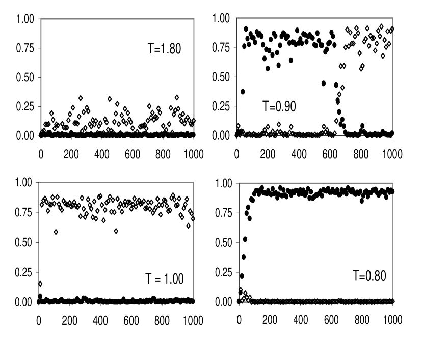
Figure 1: Time traces for $\Phi\left(0,1\right)$ ($\diamond$) and $\Phi\left(1,0\right)$ ($\bullet$) vs time (in units of 400 MCS), at four different temperatures for $q=0.425$.

The results of our simulation study are summarized in Fig. 2 which shows the phase diagram in the $q$-$T$ plane, for a $40\times 40$ system. As $q$ decreases from $0.5$ to $0$, the number of negatively charged particles increases from $0$ to $400$. To locate and distinguish continuous and first order transitions, we monitor time traces of the order parameters and extract their fluctuations, i.e., $\left\langle\Phi^{2}\left(1,0\right)\right\rangle-\left\langle\Phi\left(1,0\right)\right\rangle^{2}$ and $\left\langle\Phi^{2}\left(0,1\right)\right\rangle-\left\langle\Phi\left(0,1\right)\right\rangle^{2}$. Crossing a continuous transition, the appropriate order parameter rises smoothly from the noise, accompanied by a peak in its fluctuations. For example, at $q=0.425$, the fluctuations of the $\left(0,1\right)$ mode peak at $T=1.80\pm 0.05$, whence we use this value to (approximately) locate the transition. Proceeding in this manner, we find two lines of continuous transitions, separating the disordered phase from two different ordered phases: For $0.50\geq q\geq$ $0.46$, the disordered (D) phase becomes unstable with respect to a parallel strip (PS) as in the KLS model, while for $q\leq$ $0.45$ the system orders into the transverse strip (TS) associated with the blocking transition. However, the parallel strip reemerges, as the true low-temperature configuration: A line of first order transitions begins at $q\simeq 0.46$, $T\simeq 1.1$, extending to smaller $q$’s and $T$’s. This line separates two ordered phases: transverse strips which persist at higher temperatures, and parallel strips at lower $T$’s. Near this line, time traces of the order parameters show metastability and hysteresis. To separate stable from metastable configurations (to the accuracy of our simulations), we analyzed long runs up to $2.4\times 10^{6}$ MCS, starting from different initial configurations. For $q=0.425$, a sharp transition is easily located at $T=0.84\pm 0.01$. This becomes more difficult as $q$ increases since the continuous and first order lines approach one another and the first order character of the lower transition weakens. For smaller $q$, the first order transition shifts to such low temperatures that metastable states are effectively frozen on the time scales of our simulations.

./LS_fig2.eps

Figure 2: Phase diagram for a $40\times 40$ system in the $q,T$ plane, for $E=2$. The D-PS ($\diamond$) and D-TS ($\triangle$) transition lines are second order. The PS and TS phases are separated by first order transitions ($\circ$). The junction of the three lines marks the bicritical point.

Provided our qualitative picture is confirmed by further tests, the junction of the first and second order lines, at $q\simeq 0.46$, $T\simeq 1.1,$ is a non-equilibrium bicritical point. In fact, the system shows markedly different behavior at $q=0.45$ and $q=0.46$. At $q=0.46$ the order parameter signalling transverse strips, $\left\langle\Phi\left(0,1\right)\right\rangle$, reaches a maximum value of just $0.09$ at $T=1.2$, in stark contrast to a maximum value of $0.33$ at $T=1.1$ if $q=0.45$. Moreover, the $q=0.45$ system clearly shows a lower transition with signs of metastability, while none is observed at $q=0.46$. While it is quite remarkable that changing the sign of just eight particles makes such a difference, we emphasize that $q=0.45$ corresponds to precisely one full row of negative particles in a $40\times 40$ system while $q=0.46$ results only in a partially filled row ($32$ negative charges).

Conclusions. We have simulated a lattice gas, consisting of two oppositely charged particle species and holes subject to an “electric” field. The particles attract one another, independent of charge. This model interpolates between two well-studied limits: the KLS model [2] which has just a single species, and the high-field, high-temperature version of this model [9] where the interactions are irrelevant. Both limits exhibit order-disorder transitions, characterized however, by different ordered phases: a density-segregated strip parallel to the drive in the KLS limit, and a density- and charge-segregated strip transverse to $E$ for the two-species limit. Here, we have mapped out the phase diagram for an intermediate value of the drive, where both ordered phases are observed in different regions of parameter space. Lines of first and second order transitions, joined at a bicritical point, demarkate their stability domains.

We conclude with some remarks on work in progress [16] and open questions. Clearly, we have explored only a limited portion of the huge parameter space. Moreover, a systematic finite-size scaling analysis is needed to obtain a better estimate of the transition lines and to extract the critical properties of the continuous transitions. Preliminary studies show that the mean features of our phase diagram are independent of system size. Analytic work, ranging from mean-field to full-fledged renormalized field theory, should provide further insights. A particularly intriguing question is how $q$ and $E$ should scale with the lattice dimensions. If both are held fixed when performing the standard finite size analysis for the KLS model, the blocking transition will eventually supersede the KLS transition: a fixed charge density corresponding to a single row in a square system becomes several rows thick in a “long skinny” system. Clearly, much remains to be explored before this rich system is understood in detail.

Acknowledgements. We thank R.K.P. Zia, R.J. Astalos and U.C. Täuber for helpful discussions. Partial support from the National Science Foundation through DMR-0088451 is gratefully acknowledged.

References

References

- [1] Schmittmann B and Zia R K P 1995 Phase Transitions and Critical Phenomena vol 17, ed C Domb and J L Lebowitz (London: Academic)
- [2] Katz S, Lebowitz J L and Spohn H 1983 Phys. Rev. B28 1655 and 1984 J. Stat. Phys. 34 497
- [3] Ising E 1925 Z. Physik 31 253; McCoy B M and Wu T T 1973 The Two-dimensional Ising Model (Cambridge, Mass: Harvard Univ. Press)
- [4] See, e.g., Chandra S 1981 Superionic Solids. Principles and Applications (Amsterdam: North Holland)
- [5] Janssen H K and Schmittmann B 1986 Z. Phys B64 503; Leung K-t and Cardy J L 1986 J. Stat. Phys. 44 567 and 45 1087 (erratum)
- [6] Wang J-S 1996 J. Stat. Phys 82 1409; Leung K -t and Wang J -S 1999 Int. J. Mod. Phys. C10 853; Caracciolo S, Gambassi A, Gubinelli M, Pelissetto A cond-mat/0106221.
- [7] Leung K-t, 1991 Phys. Rev. Lett. 66 453 and 1992 Int. J. Mod. Phys. C3 367
- [8] Zhang M Q, Wang J-S, Lebowitz J L and Vallès J L 1988 J. Stat. Phys. 52 1461; Garrido P L, Lebowitz J L, Maes C and Spohn H 1990 Phys. Rev. A42 1954; Grinstein G 1991 J. Appl. Phys. 69 5441; Schmittmann B and Zia R K P 1998 J. Stat. Phys. 91 525
- [9] Schmittmann B, Hwang K and Zia R K P 1992 Europhys. Lett. 19 19
- [10] Vilfan I, Zia R K P and Schmittmann B 1994 Phys. Rev. Lett. 73 2071
- [11] Korniss G, Schmittmann B and Zia R K P 1995 Europhys. Lett. 32, 49 and 1996 J. Stat. Phys. 86 721
- [12] Leung K-t and Zia R K P 1997 Phys. Rev. E56 308
- [13] Brookings T and Zia R K P, private communication
- [14] For a review, see Chowdhury D, Santen L, and Schadschneider A 2000 Phys. Rep. 329 199
- [15] Metropolis N, Rosenbluth A W, Rosenbluth M M, Teller A H and Teller E 1953 J. Chem. Phys. 21 1087
- [16] Lyman E and Schmittmann B, unpublished