Correlation length by measuring empty space in simulated aggregates

Abstract

We examine the geometry of the spaces between particles in diffusion-limited cluster aggregation, a numerical model of aggregating suspensions. Computing the distribution of distances from each point to the nearest particle, we show that it has a scaled form independent of the concentration $\phi$, for both two- (2D) and three-dimensional (3D) model gels at low $\phi$. The mean remoteness is proportional to the density-density correlation length of the gel, $\xi$, allowing a more precise measurement of $\xi$ than by other methods. A simple analytical form for the scaled remoteness distribution is developed, highlighting the geometrical information content of the data. We show that the second moment of the distribution gives a useful estimate of the permeability of porous media.

PACS: 61.43.Hv, 82.70.Gg, 47.55.Mh, 02.70.-c

Substantial attention has been paid to cluster-cluster aggregation as a computational model of gelation in colloidal suspensions, aerogels, aggregating emulsions, etc. [1]. There is a large literature analysing the structure of individual aggregates, in terms of fractal geometry [2, 3]. However it is now properly understood [1, 4] that, in irreversibly aggregating systems at non-zero particle concentration $\phi$, clusters, while fractal at intermediate length scales, must inevitably become space-filling at the largest scales, as clusters pack to form a ‘gel’ with a well defined correlation length $\xi$. Direct analysis of the gel structure remains rare [5], although it is fundamental to a gel’s macroscopic physical properties. Colloidal gels and aerogels are porous media and, as such, the geometry of their ‘pores’ or vacancies is of prime importance, influencing the flow of permeating solvents and gel stability under external stresses such as gravity [6, 7]. Here, using the diffusion-limited cluster aggregation (DLCA) model [2], we examine the structure of the space inside the porous gel. DLCA is perhaps the simplest realistic model of aggregation in colloidal suspensions, and has been shown to qualitatively reproduce many features of experimental systems [1, 9, 10]. We show that examination of the void structure in the simulated gel leads to a measure of the correlation length $\xi$ of unprecedented precision, while the scaling with $\phi$ also gives an estimate of the cluster fractal dimension at scales smaller than $\xi$. We further find that, at low $\phi$, the pore structure is independent of $\phi$, i.e. DLCA particle gels have statistically identical structure regardless of particle concentration.

In fractal aggregates, there is no single well-defined pore size, since spaces of all sizes are present. To investigate the distribution of void sizes we require a suitable measure; but it is difficult to avoid some arbitrariness in delineating the extent of a void [11, 12]. Marine cartographers face a similar problem: where does one sea end and the next begin? We bypass the problem as follows. If an adventurer adrift in a boat sights land nearby, (s)he cannot be sure whether (s)he is on a small lake, or near the edge of a large ocean. However, if (s)he knows that the nearest land is far away, (s)he can infer the existence of a large body of water. Hence information on the distribution of void sizes can be gained by measuring the remoteness, i.e. the distance to the nearest particle, of all points in an aggregated system. This distribution of remoteness should not be interpreted, as in Ref. [13], as the distribution of void sizes. The former is only an indirect measure of the latter.

The DLCA algorithm is implemented as follows. A square (2D) or cubic (3D) grid, with periodic boundary conditions, is occupied by a randomized population of particles at concentration $\phi$. Each particle performs a random walk on the lattice until it finds a particle on a neighbouring site. The two then stick irreversibly. A cluster of particles thus formed continues its random walk, at a rate inversely proportional to its radius of gyration, forming ever larger aggregates on contact with neighbouring clusters. The growing flocs have a fractal geometry characterised by a dimension $d_{f}$ which is lower than the space dimension $d$, so that, on the scale of a cluster of ‘mass’ $M$ and radius $r$, the mean concentration ($\sim M/r^{d}\sim r^{d_{f}-d}$) decreases as the cluster grows. When the clusters grow to such a size ($\xi$) that their mean concentration ($\sim\xi^{d_{f}-d}$) matches the overall system concentration $\phi$, mass conservation demands that the clusters must fill space. Assuming a concentration-independent fractal dimension (evidenced in the limit of low $\phi$ [8, 10]), the correlation length in the ‘gels’ varies as $\xi\propto\phi^{-1/(d-d_{f})}$. To avoid artifacts in the simulations, the correlation length $\xi$ must be both significantly larger than the lattice parameter $a$, and smaller [13] than the system size $L$, $L\gg\xi\gg a$.

We analyse the ‘gel’ structure after all particles have aggregated. The fact that the particle positions are confined to the lattice is irrelevant when finding the distribution of remoteness; we visit all points in the system, and measure the Euclidean distance to the nearest particle (contrast Ref. [12]). For each gel, we compile a histogram of remoteness $h(R)$, which is normalized so that $h(R)\,\mbox{d}R$ is the probability that a point chosen at random has a remoteness in the range $R\pm\mbox{d}R/2$. It is significant that we find $h(R)$ to be normalizable. This is not the case for

similar analyses of isolated fractal clusters [11, 12, 14], where an artificial boundary must be imposed as the empty space surrounding a cluster is, in principle, limitless. The distributions we measure contain a natural cut-off, revealing that no points in the system are more remote than some finite distance.

Given the hypothesis that the correlation length is the only relevant length scale present, the cut-off distance must be a fixed fraction of $\xi$, as must other lengths such as the mean remoteness $\langle R\rangle$. To check whether a single length scale characterises the geometry at various $\phi$, we re-scale each histogram by its mean $\langle R\rangle$, and define a scaled remoteness distribution $p(x)$ with unit mean and unit norm, by $p(x)=\langle R\rangle\,h(\langle R\rangle x)$, where $x$ is remoteness measured in units of the mean (Figs. 1 and 2 for $d=2$ and $d=3$ respectively). Points at the smallest values of $x$ are affected by grid artifacts, but otherwise, the data collapse very well onto a single master curve for each value of $d$.

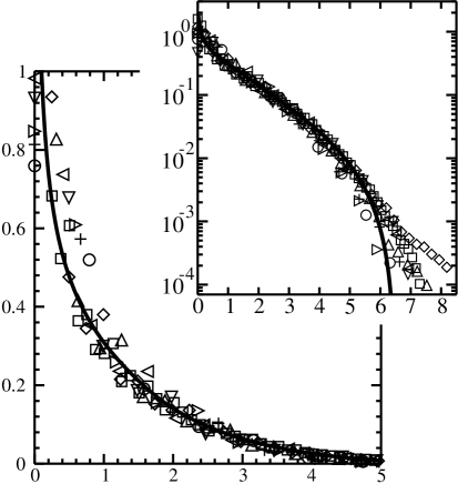
FIG. 1.: For simulations in $d=2$, the distributions, $p(x)$, of remoteness in units of the mean remoteness, for concentrations $\phi=0.10\,\Box$, $0.15\,\Diamond$, $0.17\,\triangle$, $0.20\,\triangleleft$, $0.23\,\bigtriangledown$, $0.25\,\triangleright$, $0.27\,+$, $0.30\,\bigcirc$. Solid line: one-parameter theoretical fit. Inset: The same graph on a log scale and over a wider range, making the tail of the distribution more visible.

No fitting was required to achieve the data collapse in Figs. 1 and 2, since the scale factor $\langle R\rangle$ is a well defined property of the gel. Furthermore, when we plot this length scale, the mean remoteness, against concentration $\phi$ in Fig. 3, we obtain remarkably clear power-law behaviour. As discussed, a power-law relationship between $\phi$ and any length scale proportional to $\xi$ is expected at these low concentrations, but the almost complete absence of noise was quite unforeseen. Compare equivalent plots in the literature [9] using the length scale obtained from the peak in the structure factor. We deduce that moments of the remoteness distribution are precise, noise-free measures of the length scale present in the gel.

Further confirmation that $\langle R\rangle$ is a measure of, though much smaller than, the correlation length $\xi$ comes from the gradients of the lines in Fig. 3, which are respectively $-1.67\pm 0.05$ and $-0.73\pm 0.03$ for $d=2$ and $d=3$. Given our expected gradient $-1/(d-d_{f})$, this implies a fractal dimension $d_{f}=1.40\pm 0.02$ for $d=2$, in agreement with the accepted value of 1.42 (see e.g. [1]), and $d_{f}=1.63\pm 0.05$ for $d=3$, marginally below the accepted zero-concentration value of 1.80.

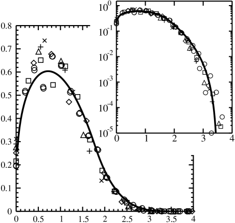
FIG. 2.: As Fig. 1, for $d=3$, at concentrations $\phi=0.02\,\bigcirc$, $0.03\,\Box$, $0.05\,\Diamond$, $0.07\,\triangle$, $0.08\,+$, $0.10\,\times$.

To find the constant of proportionality relating $\langle R\rangle$ to the more commonly used measure of the correlation length, from the peak in the structure factor at wavevector $q_{\rm max}$, we compute the ratio $\langle R\rangle/\xi=\langle R\rangle q_{\rm max}/2\pi$ for each gel, and find a constant value $0.034\pm 0.004$ for $d=2$, and $0.121\pm 0.007$ for $d=3$. We also measure higher moments of the remoteness distribution (table I).

To understand the shapes of the master curves in Figs. 1 and 2, we take as our starting point the fact that the gelled aggregate is self-similar on scales smaller than the correlation length. On some scale, we may picture the structure as a set of amorphous blobs and cavities. These cavities contain points with a range of remoteness, characterised by a normalized remoteness distribution $f(R)$. The precise form of $f(R)$ depends on the shape of the cavity. If we ‘zoom in’ to a smaller length scale $\sigma$, we notice that the blobs are themselves aggregates of blobs and cavities. By self-similarity, those smaller cavities have a normalized remoteness distribution $f(R/\sigma)/\sigma$, i.e. of the same shape as the larger cavities, but scaled down. Thus, compiling the overall histogram of remoteness, $h(R)$, we get contributions proportional to $f(R/\sigma)$ from all scales $\sigma$, up to a largest scale $\chi\sim\xi$. The magnitude of the contribution from each length scale is as yet undetermined. Let us call it $c(\sigma)$. Hence,

$$h(R)=\int_{0}^{\chi}c(\sigma)\,f(R/\sigma)\,\mbox{d}\sigma.$$ (1)

We have expressed $h(R)$, the remoteness distribution for a complex fractal aggregate, in terms of $f(R)$, the distribution of remoteness in some ‘primal’ cavity with a simple (albeit unknown), non-fractal geometry. Equation (1) may be regarded as a definition of $f(R)$.

Since the geometry is self-similar on all length scales $\sigma$ in the integration, $0\leq\sigma\leq\chi$ (ignoring a lower cut-off due to the grid), $c(\sigma)$ must be a function with no characteristic length scale, i.e. a power of $\sigma$ up to the cut-off $\chi$. In fact, we have no prior justification for the cut-off to be sharp since, in principle, scale-invariance could be lost gradually over a range of scales up to $\chi$. Nevertheless, the hypothesis will be validated by the data. We define the as yet undetermined exponent $\nu$ by $c(\sigma)=c_{0}\,\sigma^{\nu-2}$. The constant coefficient $c_{0}$ is fixed by the normalizations of $h(R)$ and $f(R)$ as $c_{0}=\nu\chi^{-\nu}$. As mentioned, the distribution of remoteness $h(R)$ is not synonymous with the distribution of void sizes. We may identify $c(\sigma)$ as the latter, while $f(R)$ contains information on the void shapes.

Recasting (1) in terms of the scaled master curve $p(x)=\langle R\rangle\,h(\langle R\rangle x)$, and putting $z=\langle R\rangle x/\sigma$, yields

$$p(x)=\frac{\nu}{x}\left(\frac{x}{x_{0}}\right)^{\nu}\int_{x/x_{0}}^{\infty}z^{-\nu}\,f(z)\,\mbox{d}z$$ (2)

where $x_{0}\equiv\chi/\langle R\rangle$, which is not a free parameter: from Eq. (1), $x_{0}^{-1}=\langle x\rangle_{f}\,\nu/(\nu+1)$ where $\langle x\rangle_{f}$ is the mean of the distribution $f(x)$. Without loss of generality, we set the size scale of the cavity described by $f(x)$ so that

FIG. 3.: Log-log plot of $\langle R\rangle/a$ vs. $\phi$ for 2D (upper set) and 3D (lower set) simulations.

$d$	$\left.\langle R^{2}\rangle^{1/2}\right/\langle R\rangle$	$\left.\langle R^{3}\rangle^{1/3}\right/\langle R\rangle$	$\left.\langle R^{4}\rangle^{1/4}\right/\langle R\rangle$	$\left.\langle R^{5}\rangle^{1/5}\right/\langle R\rangle$
2	1.42(3)	1.77(5)	2.07(8)	2.35(10)
3	1.141(9)	1.25(2)	1.35(3)	1.44(3)

TABLE I.: Ratios of the moments of the remoteness distribution, averaged over all simulations (error in last digit).

the most remote point within it is separated by unity from the nearest boundary. Hence $f(x)=0$ for $x>1$, implying $p(x)=0$ for $x>x_{0}$. So we interpret $x_{0}$ as the point on the $x$-axis of Figs. 1 and 2 at which the graph falls to zero, i.e. the value, in units of $\langle R\rangle$, of the natural upper cut-off in the remoteness distribution.

The value of the parameter $\nu$ can be calculated by examining the small-$x$ behaviour of Eq. (2). An object closely related to the remoteness distribution is the Minkowsky cover [12, 14, 15], the locus of points lying within a fixed distance, $R$ say, of a fractal set. For small $R$, the volume of the Minkowsky cover grows as $R^{d-d_{f}}$ [12, 14, 15]. Our distribution $h(R)$ is proportional to the perimeter of the Minkowsky cover, i.e. the derivative of its volume with respect to $R$. Hence, we require $p(x)\propto x^{d-d_{f}-1}$ in the limit of small $x$. As $x\to 0$, the integral in Eq. (2), assuming it is convergent, tends to a constant, so that $p(x)\propto x^{\nu-1}$ and we identify $\nu=d-d_{f}$.

It remains only to determine the form of the primal distribution $f(x)$, i.e. the geometry of the basic cavity. We know it is normalized and must vanish for $x>1$. We shall discuss some further features but, because Eq. (2) already embodies many of the correct properties for a gelled aggregate, we find the results to be insensitive to the precise form of the function $f$.

Let us examine how $f(x)$ vanishes as $x$ approaches unity from below. Consider a circular cavity with unit radius in 2D, inside which are drawn contours of equal distance from the edge, i.e. concentric circles. The cavity’s remoteness distribution $f(R)$ is proportional to the length of the contour at a distance $R$ from the edge. Hence, as we approach the centre of the cavity, $R\to 1$, $f(R)$ falls linearly to zero. This would also be the case, in 2D, for a triangular cavity, or any regular polygon. In the centre (most remote part) of a 3D cavity, on the other hand, the distribution vanishes quadratically, since it is proportional to the area of an equal-remoteness surface. Hence, one might consider substituting the normalized distribution $f_{\rm trial}=(1-x)^{d-1}d$ for $0<x<1$ into Eq. (2), thus building the fractal texture from a set of regular ‘lagoons’ of all sizes. This formula was not used for the curves in Figs. 1 and 2, despite good agreement with the 2D data, as it has shortcomings in 3D. For $d=3$, $\nu\approx 1.2$ so that, as $x\to 0$, the integral in Eq. (2) diverges if $f(0)$ is finite. At small $x$, we demand $p(x)\sim x^{d-d_{f}-1}$, which requires $p$ to be an increasing function of $x$ for $d=3$, where $d_{f}\approx 1.8$. When we construct a surface of constant distance around a tree-like ‘branch’, near the branch the area of the surface must grow as the distance from the branch is increased, because the branch is convex. But the negative gradient of $f_{\rm trial}$ describes only concave lagoons. According to our data, such a function builds an adequate picture of the spaces in a 2D aggregate, since the aggregate with $d_{f}\geq 1$ is sufficient to partition 2D space into concave lagoons of all sizes. But in 3D, branches form an imperfect cage which has significant convex structure.

To acknowledge the existence of both concave and convex parts of the aggregate, we use the simplest possible function $f(x)$ that vanishes in the correct way (with a power $d-1$) both at $x=0$ and $x=1$. We construct a piecewise smooth function that is the lower envelope of two polynomials: $c_{1}x^{d-1}$ and $c_{2}(1-x)^{d-1}$ with constant coefficients $c_{1}=\beta^{1-d}d$ and $c_{2}=(1-\beta)^{1-d}d$ chosen to ensure that it is continuous and normalized. The position of the cusp where the two parts meet, at $x=\beta$, is the only free parameter of our model. The mean of this function is at $\langle x\rangle_{f}=(1+[d-1]\beta)/(d+1)$ so that we may eliminate the parameter $\beta$ in favour of $x_{0}$ which we fit to the measured value of the cutoff in the master curves.

We find best values $x_{0}=6.5\pm 1.0$ and $3.5\pm 0.2$ for $d=2$ and $3$ respectively. These one-parameter fits are the curves shown in Figs. 1 and 2. Our single formula reproduces the data very accurately both for $d=2$ and $d=3$, even in the tails of the distributions, until the data become noisy.

The second moment of $h(R)$ has a special significance to porous media. At low Reynolds’ number, the mean flow rate, $\langle u\rangle$, of a solvent of viscosity $\eta$ through a porous medium subject to a pressure drop per unit length $\nabla P$, is given by Darcy’s law [16], $\langle u\rangle=k\nabla P/\eta$, where the permeability $k$ is a squared length scale that depends only on the geometry of the porous medium. To avoid complex hydrodynamic calculations, $k$ is often estimated by the Carman-Kozeny (CK) relation [17], $k\approx(1-\phi)^{3}/5S^{2}$, in terms of the specific surface area $S$. However, since the flow velocity at any given point is not as dependent on the total surface present as it is on the distance to the nearest obstacle, the CK relation mis-calculates the porosity in materials with more than one characteristic pore size. For instance, the flow rate through a set of parallel cylindrical holes, of various radii $a$, can be calculated exactly using Poiseuille’s formula [18], yielding $k=(1-\phi)\langle a^{4}\rangle/8\langle a^{2}\rangle$, which, expressed in terms of the remoteness, is $k=3\langle R^{2}\rangle/4$. By substituting the surface area of the holes into the CK formula, one obtains $k_{\rm CK}\approx(1-\phi)\langle a^{2}\rangle/10$, which approximates the exact value only for a sharply peaked distribution of radii, for which $\langle a^{4}\rangle\approx\langle a^{2}\rangle^{2}$. The approximation fails too for a polydisperse set of parallel-sided channels, where the exact result can be expressed as $k=\langle R^{2}\rangle/2$. We therefore propose an approximate rule of thumb $k\approx 0.6\langle R^{2}\rangle$, which continues to hold for polydisperse pores and for rough surfaces while, in both cases, the CK equation fails. The new formula has been shown to yield results of the correct order of magnitude for fractal particulate gels [6]. However, like the CK equation, the new formula lacks information on pore topology, so must also fail in certain cases, e.g. where some pores are closed. There is then no alternative to a full hydrodynamic computation.

The shape of the remoteness distribution carries information on the geometry in the DLCA simulations, and confirms (by scaling onto a master curve) that, statistically speaking, all the simulations at the low concentrations considered, give rise to the same geometry: the particle gel ‘pore’ structure is independent of concentration. The mean remoteness, an easy quantity to measure in the simulations, is proportional to the correlation length (at least in the range of concentrations studied), hence giving a measure of the gel’s characteristic length scale that is considerably less noisy, and perhaps more easily determined, than other measures. The second moment of the remoteness distribution provides an estimate of the permeability of the gel. These coordinate-independent measures of real-space length scales could be applied to a range of other phenomena, such as the void geometry in reaction-limited aggregation [19] and in earlier stages of aggregation [4], or the $\phi$-dependence at higher concentrations [8] when the structure is no longer controlled solely by the zero-concentration critical phenomena.

RMLE acknowledges the support of the Royal Society and the Royal Society of Edinburgh.

REFERENCES

- [1] W. C. K. Poon and M. D. Haw, Adv. Colloid Interface Sci. 73, 71 (1997), and references therein.
- [2] P. Meakin, Phys. Rev. Lett 51, 1119 (1983); M. Kolb, R. Botet and R. Jullien, ibid 51, 1123 (1983).
- [3] T. Vicsek, ‘Fractal Growth Phenomena’, (World Scientific, Singapore, 1989).
- [4] J. C. Gimel, T. Nicolai and D. Durand, J. Sol-Gel Sci. Tech. 15, 129 (1989).
- [5] J. C. Gimel, D. Durand and T. Nicolai, Phys. Rev. B 51, 11348 (1995)
- [6] R. M. L. Evans and L. Starrs, in preparation.
- [7] P. M. Adler in ‘The fractal approach to heterogeneous chemistry’ edited by D. Avnir (John Wiley & Sons, Chichester, 1989).
- [8] M. Lach-hab, A. E. González and E. Blaisten-Barojas, Phys. Rev. E 54, 5456 (1996).
- [9] A. E. González and G. Ramírez-Santiago, Phys. Rev. Lett. 74,1238 (1995).
- [10] J. Bibette, T. G. Mason, H. Gang and D. A. Weitz, Phys. Rev. Lett. 69, 981 (1992).
- [11] C. Allain and M. Cloitre, Phys. Rev. A 44, 3552 (1991).
- [12] S. Schwarzer, S Havlin and H. E. Stanley, Phys. Rev. E 49, 1182 (1994).
- [13] A similar, but coordinate-dependent, measure of remoteness appears in F. Ehrburger-Dolle, P. M. Mors and R. Jullien, J. Colloid Interface Sci. 147, 192 (1991). We note that in the simulations at finite , so that only finite size effects were measured.
- [14] B. Dubuc, J. F. Quiniou, C. Roques-Carmes, C. Tricot and S. W. Zucker, Phys. Rev. A 39, 1500 (1989).
- [15] P. Pfeifer and M. Obert in ‘The fractal approach to heterogeneous chemistry’ edited by D. Avnir (John Wiley & Sons, Chichester, 1989).
- [16] H. P. G. Darcy, Les Fontaines Publiques de la Ville de Dijon (Dalmont, Paris, 1856).
- [17] L. M. Schwartz, N. Martys, D. P. Bentz, E. J. Garboczi and S. Torquato, Phys. Rev. E 48, 4584 (1993); A. W. Heijs and C. P. Lowe, ibid 51, 4346 (1995).
- [18] M. Reiner, Deformation, strain and flow (H. K. Lewis, London, 1950).
- [19] P. B. Warren, Phys. Rev. A 44, 7991 (1991).