Calculation of ${\bm{\Delta}}{\bf(k,}{\bm{\omega}}{\bf)}$ for a 2D t-J Cluster

Abstract

Using numerical techniques, the diagonal and off-diagonal superconducting one-electron Green’s functions are calculated for a two-dimensional (2D) t-J model on a periodic 32-site cluster at low doping. From these Green’s functions, the momentum and frequency dependence of the pairing gap $\Delta({\bf k},\omega)$ are extracted. It has $d_{x^{2}-y^{2}}$ symmetry and exhibits $\omega$-dependent structure which depend upon J/t. We find that the pairing gap persists down to small J/t values. The frequency- and momentum-dependent renormalized energy and renormalization factor are also calculated.

For the last decade, the search for superconductivity in models of strongly-correlated fermions, has been triggered by accumulating experimental evidence in favor of an unconventional (i.e. not based on the usual phonon-mediated interaction) mechanism in high-$T_{c}$ two-dimensional (2D) TK00 or ladder DR96 superconducting cuprates. Soon after the discovery of the layered cuprates, it was proposed that the Hubbard model And87 and its strong coupling limit, the t-J model ZR88 , captured the generic features of these materials. Early RPA MSV86 ; SLH86 and Gutzwiller variational calculations GJR87 supported the notion that the doped state would have $d_{x^{2}-y^{2}}$ pairing. Nevertheless, despite the conceptual simplicity of these Hamiltonians and the results of these approximate calculations, the nature of the basic mechanism responsible for pairing as well as the actual physical properties of these models remained controvertial. In recent years, numerical calculations have provided insight into the second of these questions regarding the actual properties of these models. Specifically, Monte Carlo calculations showed that the ground states of the undoped models had long-range antiferromagnetic order HT89 ; RRY89 . Exact diagonalization studies showed that holes doped into a t-J cluster can form $d_{x^{2}-y^{2}}$ pairs Poi93 ; Leu00 . In addition, numerical calculations support the view that the doped system can have low-lying stripe domain wall states SW00 which can be stabilized by lattice anisotropies KSW01 ; BCS01 . While the static striped phase competes with superconductivity, it has been argued that the addition of a next-near-neighbor hopping WS99 or the use of periodic boundary conditions Sor01 tips the balance in favor of the $d_{x^{2}-y^{2}}$ pairing phase. The point is that a variety of numerical calculations provide evidence that indeed these models do exhibit the basic properties seen in the cuprates. However, in spite of this progress, the question regarding the nature of the basic mechanism responsible for the pairing remains open. Within the traditional BCS framework, one would look for a reflection of the pairing interaction by examining the momentum and frequency dependence of the gap $\Delta({\bf k},\omega)$. Because of the relatively short coherence length and the relatively high energy scales J and t, one can hope to learn about both the momentum and frequency dependence of $\Delta({\bf k},\omega)$ from an exact diagonalization study of a cluster. Here we present a numerical study aimed at doing this for the t-J model and obtain the first results for the $\omega$-dependence of the gap.

The 2D t–J Hamiltonian reads,

$$H = \sum_{i,j}J_{ij}({\bf S}_{i}\cdot{\bf S}_{j}-\frac{1}{4}n_{i}n_{j})$$ (1)

$$+ \sum_{i,j,\sigma}t_{ij}({\tilde{c}}_{i,\sigma}^{\dagger}{\tilde{c}}_{j,\sigma}+h.c.)$$

where the exchange integrals $J_{ij}$ and hopping terms are (for simplicity) restricted to nearest neighbor (NN) sites (called hereafter $J$ and $t$) and ${\tilde{c}}_{i,\sigma}^{\dagger}$ are projected fermion creation operators defined as $c_{i,\sigma}^{\dagger}(1-n_{i,-\sigma})$. Hereafter, unless specified otherwise, $t$ sets the energy scale. The conclusions drawn in this Letter are supported by Exact Diagonalisation (ED) studies performed on the square cluster of N=32 sites depicted in Fig. 1(a) slightly doped with up to 2 holes note1 . This finite-size system is particularly appealing since it exhibits the full local symmetries of the underlying square lattice as well as all the most symmetric ${\bf k}$-points in reciprocal space as seen in Fig. 1(b). Note that, although the hole doping is quite small, the hole occupation shown in Fig. 1(b) for a few $\bf k$-points is rather consistent with a ”large” Fermi surface.

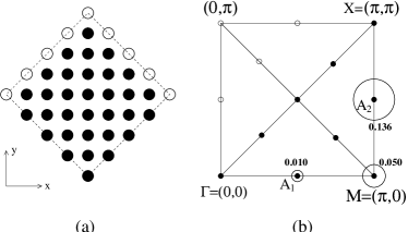
Figure 1: (a) Periodic square 32-site cluster; (b) Reciprocal space of the 32-site cluster. The area of the circles (drawn only for a few ${\bf k}$-points especially relevant to our analysis) correspond to the hole occupancies $\big{<}{\tilde{c}}_{{\bf k},\sigma}{\tilde{c}}_{{\bf k},\sigma}^{\dagger}\big{>}$ in the 2-hole GS at $J=0.3$ (whose exact values are also shown on the plot).

A superconducting ground state (GS) is characterized by Gorkov’s off-diagonal one-electron time-ordered Green function

$$F_{\bf k}(t)=-\left\langle T{\tilde{c}}_{{\bf-k},-\sigma}(t/2){\tilde{c}}_{{\bf k},\sigma}(-t/2)\right\rangle\,.$$ (2)

Close to half-filling, in a finite system, $F_{\bf k}$ can be computed from,

$${\tilde{F}}_{\bf k}(z)=\left\langle N-2|{\tilde{c}}_{{\bf-k},-\sigma}\frac{1}{z-H+{\bar{E}}_{N-1}}{\tilde{c}}_{{\bf k},\sigma}|N\right\rangle\,,$$ (3)

defined for all complex $z$ (with ${\rm Im}\,z\neq 0$). Here the number of particles in the initial $|N\big{>}$ (half-filling) and final $|N-2\big{>}$ (two-hole doped) GS differ by two, reflecting charge fluctuations in a SC state. For convenience, the energy reference ${\bar{E}}_{N-1}$ is defined as the average between the GS energies of $|N\big{>}$ and $|N-2\big{>}$. Note that these states are both spin singlets. In addition, they exhibit s-wave and d${}_{x^{2}-y^{2}}$ orbital symmetries (both of even parity) respectively. Owing to these special features, it is straightforward to show that the analytical continuation of $F_{\bf k}(\omega)$ to the real frequency axis is even in frequency and can be expressed as,

$$F({\bf k},\omega)={\tilde{F}}_{\bf k}(\omega+i\epsilon)+{\tilde{F}}_{\bf k}(-\omega+i\epsilon)\,,$$ (4)

where $\epsilon$ is a small imaginary part. The superconducting frequency-dependent gap function $\Delta({\bf k},\omega)$ is directly proportional to $F({\bf k},\omega)$ and a simple analysis shows that both functions have d${}_{x^{2}-y^{2}}$ orbital symmetry. In particular, they identically vanish on the diagonals $k_{x}=\pm k_{y}$.

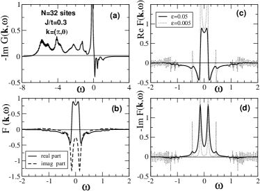
Figure 2: Diagonal and off-diagonal one-electron (time-ordered) Green functions versus frequency (in units of $t$) obtained on the cluster of Fig. 1 and an average hole doping of $3\%$; (a) $-\rm{Im}\,G({\bf k},\omega)$; (b) real and imaginary parts of $F({\bf k},\omega)$ for $\epsilon=0.05$; (c,d) comparison between the data of $\rm{Re}\,F$ and $-\rm{Im}\,F$ obtained with $\epsilon=0.05$ and with $\epsilon=0.005$.

Pairing between holes should also be reflected in the structure of the (time-ordered) diagonal Green function $G({\bf k},\omega)$. Here, it is convenient to define the finite size $G({\bf k},\omega)$ as the sum of the following electron- (i.e. occupied states for $\omega<0$) and hole-like (i.e. empty states for $\omega>0$) parts,

$$G({\bf k},\omega)=\left\langle N|{\tilde{c}}_{{\bf k},\sigma}^{\dagger}\frac{1}{\omega-i\epsilon+H-{\bar{E}}_{N-1}}{\tilde{c}}_{{\bf k},\sigma}|N\right\rangle$$ (5)

$$+ \big{<}N-2|{\tilde{c}}_{{\bf k},\sigma}\frac{1}{\omega+i\epsilon-H+{\bar{E}}_{N-1}}{\tilde{c}}_{{\bf k},\sigma}^{\dagger}|N-2\big{>}\,,$$

so that both Green functions $F$ and $G$ have the same set of energy poles. Here, the well-known continued-fraction method used to compute diagonal correlation functions such as $G({\bf k},\omega)$ is extended to deal with off-diagonal ones such as $F({\bf k},\omega)$ OSEM94 ; continued_frac . Data are shown in Fig. 2(a-d). The spectral density $\rm{Im}\,G({\bf k},\omega)$ exhibits sharp quasi-particle-like peaks both above and below the Fermi level ($\omega=0$). Contrary to $G({\bf k},\omega)$, $F({\bf k},\omega)$ has a significant amplitude only at low energy, typically for $|\omega|<4J$ as seen in Fig. 2(b), reflecting the energy scale of the pairing interaction. Note that, due to the discreteness of the low energy spectrum of the cluster, a finite value of $\epsilon$ is necessary to wipe out the irrelevant fast oscillations of the $F$ (or $G$) Green functions (see e.g. Fig. 2(c-d)). However, the static limit $\omega\rightarrow 0$ (together with $\epsilon\rightarrow 0$) is perfectly controled and has a physical meaning.

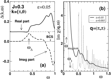
Figure 3: (a) Real and imaginary components of the frequency-dependent gap function (in units of $t$) at low energies. (b) Dynamical spin structure factor in the 2 hole-doped 32-site cluster. The positions in energy of the first pole (magnon) and of the mean value of the spectrum are indicated by arrows.

The frequency-dependent gap function $\Delta({\bf k},\omega)$ can be extracted from the knowledge of the Green functions by assuming generic forms of a SC GS schrieffer at low energies,

$$G({\bf k},\omega) = z({\bf k},\omega)\frac{\omega+\epsilon({\bf k},\omega)}{\omega^{2}-(\epsilon({\bf k},\omega)^{2}+\Delta({\bf k},\omega)^{2})+i\epsilon},$$

$$F({\bf k},\omega) = z({\bf k},\omega)\frac{\Delta({\bf k},\omega)}{\omega^{2}-(\epsilon({\bf k},\omega)^{2}+\Delta({\bf k},\omega)^{2})+i\epsilon},$$ (6)

where $z({\bf k},\omega)$ and $\epsilon({\bf k},\omega)$ are the inverse renormalization parameter and the renormalized energy (containing the energy shift) respectively. In the BCS limit, the renormalized energy $\epsilon({\bf k},\omega)\equiv\epsilon_{\bf k}$ and the gap function $\Delta({\bf k},\omega)\equiv\Delta_{\bf k}$ do not depend on frequency (and $z({\bf k},\omega)=1$) so that $F({\bf k},\omega)$ exhibits only two poles at $\pm(\epsilon_{\bf k}^{2}+\Delta_{\bf k}^{2})^{1/2}$. However, it is necessary to assume an explicitely frequency dependence of the gap function in order to reproduce the secondary peaks seen in Fig. 2(d). Using the parity of $\epsilon({\bf k},\omega)$ and $\Delta({\bf k},\omega)$ in the vicinity of the real frequency axis one gets,

$$\Delta({\bf k},\omega)=\frac{2\omega F({\bf k},\omega)}{G({\bf k},\omega)-G({\bf k},-\omega)}$$ (7)

Thus, from a numerical calculation of $G({\bf k},\omega)$ and $F({\bf k},\omega)$, one can obtain $\Delta({\bf k},\omega)$.

Results for $\Delta({\bf k},\omega)$ with ${\bf k}=(\pi,0)$ at the $M$ point, are shown in Fig. 3(a). Despite the limited resolution in frequency of the ED data, $\Delta({\bf k},\omega)$ exhibits dynamic structure on a scale of energies several times J. We believe that finite-size effects have increased the onset frequency $\omega_{\Delta}$ and that the corresponding time $2\pi/\omega_{\Delta}$ should be viewed as a lower bound of the characteristic time scale of the pairing interaction. For comparison, the dynamic spin structure factor $Im\chi({\bf q},\omega)$ for the 2-hole doped 32-site cluster with ${\bf q}=(\pi,\pi)$ is shown in Fig. 3(b).

The quasi-particle gap at the gap edge, where $\epsilon({\bf k},0)=0$, is determined from the self-consistent solution of

$$Re\Delta({\bf k},\omega=\Delta_{\bf k})=\Delta_{\bf k}$$ (8)

As shown in Fig. 3(a), $\Delta({\bf k},\omega)$ is real and essential constant over an energy region larger than the gap. Furthermore, as we will see, $\epsilon({\bf k},0)$ for ${\bf k}=(\pi,0)$ is small so that $\Delta_{\bf k}$ is to a good approximation given by $\Delta({\bf k},0)$. For ${\bf k}=(\pi,0)$, the zero frequency limit of the gap function $\Delta({\bf k},\omega\to 0)$ (which is purely real) computed by numerically taking the $\omega$ and $\epsilon\to 0$ limits of eq. (7) note2 is plotted versus J in Fig. 4(a). In Fig. 4(b) the static $\omega=0$ value of the renormalization energy $\epsilon({\bf k},0)$, the renormalization factor $z({\bf k},\omega=0)$, and the equal-time pair amplitude $\langle{\tilde{c}}^{\dagger}_{-{\bf k},-\sigma}{\tilde{c}}^{\dagger}_{{\bf k}\sigma}\rangle$ for ${\bf k}=(\pi,0)$ versus J are also shown note2_bis . The values of $\Delta(k,0)$ and $z(k,0)$ are in good agreement with the results Ohta, et. al OSEM94 found by fitting their numerical t-J $4\times 4$ and $\sqrt{18}\times\sqrt{18}$ cluster calculations to a BCS quasi-particle form in which the frequency dependence of $\Delta$ and $z$ were neglected. They found that the magnitude of the gap at the antimode varies as 0.25J to 0.3J at low doping and as seen in Fig. 4(a) we find $\Delta(k,0)\sim 0.3J$. It is interesting to note that the data for $\Delta(k,0)$ in Fig. 4(a) do not show any lower bound of J in contrast to the pair binding energy Poi93 ; Leu00 . The spin structure factor is plotted in Fig. 3(b) showing a low energy peak (magnon) and a higher energy background that could be connected to the structures in the gap function at an energy $\sim J$. For comparison, the magnon energy and the mean-value note3 of the spin spectral weight are plotted in Fig. 4(a) together with the zero-frequency gap and the onset frequency $\omega_{\Delta}$ in the gap function. While the similarities in the J-dependence of these quantities suggest that the dynamics underlying the pairing mechanism is related to the spin fluctuations, further work on other clusters, such as 2-leg ladders, are needed to sort out the influence of finite-size effects.

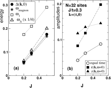
Figure 4: (a) Zero-frequency gap and typical frequency $\omega_{\Delta}$ (divided by 4) of the gap function (in units of $t$) plotted vs J. For comparison, the magnon energy and the mean-value $\omega_{1}$ of the spin structure factor (see Fig. 3(b) is also shown. (b) Equal-time pair amplitude $\langle{\tilde{c}}^{\dagger}_{-{\bf k},-\sigma}{\tilde{c}}^{\dagger}_{{\bf k},\sigma}\rangle$ calculated at momentum ${\bf k}=(\pi,0)$ vs $J/t$. The renormalized energy $\epsilon({\bf k},0)$ (in units of $t$) and the renormalization parameter $z({\bf k},\omega=0)$ are also shown as filled squares and triangles, respectively.

Table 1: Static limit ($\omega=0$) of the gap function, the renormalized energy and the renormalization parameter at a few ${\bf k}$-points away from the nodes and for $J/t=0.3$.

${\bf k}$-points	$\Delta({\bf k},0)$	$\epsilon({\bf k},0)$	$z({\bf k},0)$
$(\pi/2,0)$	0.064958	0.20260	0.21221
$(\pi,0)$	0.095641	0.11867	0.13542
$(\pi,\pi/2)$	0.186100	0.08895	0.12855

We conclude this investigation with a further discussion of the parameters which enter eq. (6). Note that since these parameters depend upon both ${\bf k}$ and $\omega$, the static $\omega=0$ results which we will discuss are near the energy shell only for ${\bf k}$ values near the fermi surface and for $\Delta_{\bf k}$ small compared to the characteristic frequency variations set by J. In fact, even trying to select ${\bf k}$-points near the “Fermi surface” defined by $\epsilon({\bf k},0)=0$ requires some care since the Fermi surface (FS) cannot be exactly defined on a finite cluster, especially for a small number of holes. However, the smooth variation of the hole occupancy in the BZ [see Fig. 1(b)] suggests that this system should still pick up features of a slightly doped AF with a large FS. With this in mind, the static limit of the renormalized energy $\epsilon({\bf k},0)$ and the renormalization parameter $z({\bf k},0)$ were obtained from the calculated $\epsilon,\omega\to 0$ limits of $G({\bf k},0)$, $F({\bf k},0)$, and $\Delta({\bf k},0)$ by using eq. (6) for $\omega=0$. These are tabulated for values of ${\bf k}$ both near the nominal FS and away from it in Table 1. The renormalized energy $\epsilon({\bf k},0)$ has roughly the energy scale of the quasi-particle-like energy poles at the available momenta of the BZ. The small value of $\epsilon({\bf k},0)$ given by our analysis for ${\bf k}=(\pi,0)$ show that the excitation that we are probing is relatively close to the FS (defined here as having $\epsilon({\bf k},0)=0$. Note also that the weight $z({\bf k},0)$ of these excitations is small $(\approx J/2)$ compared to the large incoherent background [see Fig. 2(a)]. Its J-dependence plotted in Fig. 4(b) is consistent with the $J^{\alpha}$ power-law behavior found previously in earlier calculations of a single hole propagating in an AF background PSZ93 .

- (1) C.C. Tsuei and J.R. Kirtley, Rev. Mod. Phys. 72, 969 (2000).
- (2) E. Dagotto and T.M. Rice, Science 271, 618 (1996).
- (3) P.W. Anderson, Science 235, 1196 (1987).
- (4) F.C. Zhang and T.M. Rice, Phys. Rev. B 37, 3759 (1988).
- (5) K. Miyaki, S. Schmitt-Rink, C.M. Varma, Phys. Rev. B 34, 6554 (1986).
- (6) D.J. Scalapino, E. Loh, and J. Hirsch, Phys. Rev. B 34, 8190 (1986).
- (7) C. Gros, R. Joynt, and T.M. Rice, Z. Phys. B 68, 425 (1987).
- (8) J.E. Hirsch and S. Tang, Phys. Rev. Lett. 62, 591 (1989).
- (9) J.D. Reger, J.A. Riera, and A.P. Young, J. of Phys.: CM 1, 1855 (1989).
- (10) D. Poilblanc, Phys. Rev. B 48, 3368 (1993); Phys. Rev. B 49, 1477 (1994).
- (11) P.W. Leung, Phys. Rev. B 62, R6112 (2000).
- (12) D.J. Scalapino and S.R. White, Physica C 341–348, 367 (2000).
- (13) A.P. Kampf, D.J. Scalapino, and S.R. White, Phys. Rev. B 64, 52509 (2001).
- (14) F. Becca, L. Capriottie, and S. Sorella; cond-mat/0108198.
- (15) S.R. White and D.J. Scalapino, Phys. Rev. B 60, R753 (1999).
- (16) S. Sorella, et. al; cond-mat/0110460.
- (17) We thank P.W. Leung for providing us with the 2 hole GS energy (see Ref. Leu00 ) which we have reproduced.
- (18) Y. Ohta, T. Shimozato, R. Eder, and S. Maekawa, Phys. Rev. Lett. 73, 324 (1994).
- (19) Further details of our calculation will be published elsewhere.
- (20) J.R. Schrieffer, Theory of Superconductivity (Benjamin, NY 1964).
- (21) Formally eq. (7) gives .
- (22) Note that the equal-time pair amplitude equals the integrated weight .
- (23) For a normalized distribution , we define .
- (24) D. Poilblanc, H.J. Schulz, T. Ziman, Phys. Rev. B 47, 3268 (1993) and references therein.