Electron-phonon scattering at the intersection of two Landau levels

Abstract

We predict a double-resonant feature in the magnetic field dependence of the phonon-mediated longitudinal conductivity $\sigma_{xx}$ of a two-subband quasi-two-dimensional electron system in a quantizing magnetic field. The two sharp peaks in $\sigma_{xx}$ appear when the energy separation between two Landau levels belonging to different size-quantization subbands is favorable for acoustic-phonon transitions. One-phonon and two-phonon mechanisms of electron conductivity are calculated and mutually compared. The phonon-mediated interaction between the intersecting Landau levels is considered and no avoided crossing is found at thermal equilibrium.

I INTRODUCTION

The acoustic phonon scattering of electrons in two-dimensional (2D) systems in quantizing magnetic fields has been extensively studied for the last three decades. The peculiar density of states of the 2D electrons in a transversal magnetic field $B$ produces a suppresion of the electron-phonon stattering rate at strong magnetic fields [1, 2], at which the so called inelasticity parameter $\eta=s/\lambda\omega_{c}$ is less than unity, here $s$ is the sound velocity, $\lambda=\sqrt{\hbar/eB}$ is the magnetic length, and $\omega_{c}=eB/m$ is the cyclotron frequency. A detailed analysis of the acoustic phonon emission and absorption spectra in 2D electron systems has been carried out in connection with developing a phonon absorption spectroscopy [3, 4, 5], which is used to investigate the states of electronic matter in both integer and fractional quantum Hall effects. It was also noticed that, at a certain stage of supression of the one-phonon inter-Landau-level transition, the two-phonon transition dominates the electron relaxation rate [6]. However, in a two-subband system, the electron relaxation rate can still be due to the one-phonon transitions occurring between Landau levels of different size-quantization subbands. An oscillatory behavior of the electron lifetime was found in a two-subband system [7].

In this paper we focus on an intersection of two Landau levels belonging to different size-quantization subbands of a two-dimensional electron gas in a transversal magnetic field $B$ (see Fig. 1). The electron density is chosen so that there are enough electrons to fill only one Landau level out of the two at the intersection point. Despite the general suppression due to small $\eta$, we find that, at an energy separation between the two Landau levels of the order of the characteristic acoustic-phonon energy $T_{\lambda}=\hbar s/\lambda$, the electron-phonon scattering is significantly enhanced. In what follows, we neglect the effects related to the Coulomb interaction between the electrons. These effects change significantly the results at low temperatures [8]. The virtue of the considered structure, from the point of view of electron-phonon scattering, is that an enhancement of the dissipative conductivity $\sigma_{xx}$ arises on the background of its strong overall suppression. This enhancement can be understood from the following physical consideration.

At the intersection of two Landau levels, say level $\ell=0$ of the upper subband and level $\ell=1$ of the lower subband, the matrix element of the electron-phonon interaction requires a phonon momentum $q\sim 1/\lambda$ for the most efficient transition. Note that two Landau levels can be intersected at a magnitude of $B$ corresponding to $\lambda\sim a$, where $a$ is the characteristic width of the quantum well confining the two-dimensional electron gas. This results in $q_{z}\sim q_{\bot}\sim 1/\lambda$, where $q_{z}$ and $q_{\bot}$ are the perpendicular and in-plane components of the phonon momentum, respectively. On the other hand, the energy conservation law requires that the phonon energy $\hbar\omega_{\bf q}$ matches the energy separation between the two Landau levels $\Omega=|{\cal E}_{\ell=0}-{\cal E}_{\ell=1}|$. For acoustic phonons, we have $\omega_{\bf q}=sq$, and if combined with the momentum requirement, two resonances are obtained, one on each side of the crossing point, corresponding to $\Omega\simeq\hbar s/\lambda\equiv T_{\lambda}$. At each resonance the electron-phonon scattering is significantly enhanced, owing to the one-phonon transitions.

It is worth noting that a simultaneous intersection of two Landau levels with the Fermi level leads to a missing quantum Hall effect plateau as expected from a single-subband consideration. Such intersections occur repeatedly with decreasing $B$, if the electron density per spin orientation $n_{2D}=n_{c}(1+(2p-1)/q)$, where $p$, $q$ are natural numbers, and $n_{c}=mE_{12}/2\pi\hbar^{2}$, with $E_{12}$ being the energy separation between the two size-quantization subbands. However, if the Coulomb interaction between the electrons is taken into account, a new energy gap emerges at the intersection point [8].

An enhancement of the electron scattering in a two-subband system occurs also at zero magnetic field, when the second size-quantization subband starts being filled with electrons. This effect can be viewed in terms of a Lifshitz topological transition of the Fermi surface, which is well known for the 3D case [9]. The 2D case of this transition was considered in Ref. [10], where the electron scattering occured on a random potential of impurities. At $B\neq 0$, one can hardly speak of a Fermi surface. However, we refer the peculiar behaviour of $\sigma_{xx}$ in our case to the same origin – a strong variation in the density of states at the Fermi level. The case considered in this paper has the advantage of more pronunced anomalies.

An experimental realization of the above described situation can be acheived in GaAs/AlGaAs heterojunctions. Usually, the donor supply of the electrons into the 2D layer is not sufficient to achieve filling of the second size-quantization subband. However, a significant increase in the concentration can be achieved by illuminating the sample with photons of energy close to the band gap of GaAs. The photoexcited electrons come either from the DX centers in the AlGaAs layer [11] or from the valence band of the bulk GaAs producing a charge separation at the interface [12]. Furthermore, the 2D electron concentration can be tuned within a large range using the method of continuous photoexcitation [13]. Population of the second subband of size quantisation in a magnetic field has been observed in a number of experiments related to magneto-optical studies of the integer and fractional quantum Hall effects [14]^-[16].

In this paper we consider only scattering of electrons by phonons, although in a real 2D system the main contribution into $\sigma_{xx}$ at low temperatures comes from the scattering of electrons by the impurity potential. This was extensively studied in connection with the integer quantum Hall effect. However, since the electron-phonon coupling constant $\alpha\sim B$, the phonon-induced $\sigma_{xx}$, at high enough magnetic fields, may be comparable with the impurity induced $\sigma_{xx}$.

II GENERAL RELATIONS

We consider an electron gas in a quantum well, formed by a confining potential $V(z)$, in a strong magnetic field $B$ directed along the axis $z$. In the Landau gauge the vector potential ${\bf A}=(0,xB,0)$, and the electron can be characterised by the center of orbit coordinate $X$. The energy spectrum of the electron, ${\cal E}_{n\ell}=E_{n}+\hbar\omega_{c}(\ell+1/2)$, consists of the size quantization energy $E_{n}$ and the magnetic quantization energy, described by the Landau level number $\ell$. The acoustic phonons, with dispersion $\omega_{{\bf q}\,j}$, interact with the electrons via both deformation potential (DP) and piezoelectric (PE) mechanisms. We shall restrict ourselves to the isotropic Debye approximation in which the phonon modes fall into a branch of longitudinal (LA) phonons ($j=1$) and two branches of transversal (TA) phonons ($j=2,3$). This seems to be a good approximation for phonons at thermal equilibrium, in contrast with the case of balistic phonon propagation, where the anysotropy gives rise to self-focusing effects [18]. For GaAs, it follows that the DP mechanism couples electrons only with LA phonons. We assume that acoustic phonons are the only sourse of scattering for the electrons in the well, neglecting the effects of interface roughness and random potential of impurities, as well as the presence of optical phonon modes. This assumption is valid for fairly pure samples at temperatures below the optical phonon energy. We also suppose the acoustical phonons to be three dimentional, neglecting the effects of interface phonons. The electrons are considered spinless. The spin degeneracy can be easily accounted for at the final stage of calculation. Electron scattering by phonons is spin preserving, and the results for the conductivity will differ only by a factor of 2.

The system of interacting electron and phonon gases is described by the following second quantized Hamiltonian

$$H=H_{0}+H_{int}\;\;,$$ (1)

with

$$H_{0}=\sum_{n\,\ell\,X}{{\cal E}_{n\ell}C^{{\dagger}}_{n\ell X}C_{n\ell X}}\;+\sum_{{\bf q}\,j}{\hbar\omega_{{\bf q}\,j}(b^{{\dagger}}_{{\bf q}\,j}b_{{\bf q}\,j}+1/2)}\;\;,$$ (2)

and

$$H_{int}=-\sum_{n\ell n^{\prime}\ell^{\prime}\atop{\bf q}\,jX}M^{{\bf q}\,j}_{X}\!\!\,\left(\!\!\begin{array}[]{c}n^{\prime}\ell^{\prime}\vspace{-8 pt}\\ n\>\ell\end{array}\!\!\right)\,(b^{{\dagger}}_{-{\bf q}\,j}+b_{{\bf q}\,j})C^{{\dagger}}_{n^{\prime}\ell^{\prime}X-\lambda^{2}q_{y}}C_{n\ell X}\;\;.$$ (3)

Here $C^{{\dagger}}_{n\ell X}$, $C_{n\ell X}$ and $b^{{\dagger}}_{{\bf q}\,j}$, $b_{{\bf q}\,j}$ stand for the creation and annihilation operators of the electron and phonon respectively. The matrix element of electron-phonon interaction is given by the formula

$$M^{{\bf q}\,j}_{X}\!\!\,\left(\!\!\begin{array}[]{c}n^{\prime}\ell^{\prime}\vspace{-8 pt}\\ n\>\ell\end{array}\!\!\right)=(e\beta_{{\bf q}\,j}-iq\Xi_{{\bf q}\,j})\sqrt{\frac{\hbar}{2\omega_{{\bf q}j}\,\rho_{c}V_{3d}}}F_{nn^{\prime}}(q_{z})\Omega_{\ell\ell^{\prime}}(q_{\bot})e^{iq_{x}(X-\lambda^{2}q_{y}/2)+i\varphi(\ell-\ell^{\prime})}\;\;,$$ (4)

where $q_{\bot}=\sqrt{q_{x}^{2}+q_{y}^{2}}$ is the value of the in-plane component of the phonon wave vector q, and $\varphi$ is the polar angle of ${\bf q_{\bot}}$, counted from the $x$-axis. The sample volume and density are noted by $V_{3d}$ and $\rho_{c}$, respectively. The factor $\Omega_{\ell\ell^{\prime}}(q_{\bot})$ for $\ell\geq\ell^{\prime}$ reads

$$\Omega_{\ell\ell^{\prime}}(q_{\bot})=i^{\ell-\ell^{\prime}}\left(\frac{\ell^{\prime}!}{\ell!}\right)^{1/2}e^{-\chi^{2}/2}\chi^{\ell-\ell^{\prime}}L^{\ell-\ell^{\prime}}_{\ell^{\prime}}(\chi^{2})\;\;,$$ (5)

$$\chi^{2}=\lambda^{2}q_{\bot}^{2}/2\;\;,$$

where $L_{n}^{m}(x)$ are the associated Laguerre polynomials. For $\ell<\ell^{\prime}$, $\Omega_{\ell\ell^{\prime}}(q_{\bot})$ is obtained from Eq. (5) by interchanging the indices $\ell$ and $\ell^{\prime}$ in the right-hand-side of (5). The parameter $\Xi_{{\bf q}\,j}$ is introduced as follows,

$$\Xi_{{\bf q}\,j}=\frac{1}{2q}\Xi^{\mu\nu}(q_{\mu}e^{(j)}_{\nu}({\bf q})+q_{\nu}e^{(j)}_{\mu}({\bf q}))\;\;,$$ (6)

$\Xi^{\mu\nu}$ being the deformation potential tensor and ${\bf e}^{(j)}({\bf q})$ the polarization vector of the $j$-th phonon branch. For GaAs, it reduces to $\Xi_{{\bf q}\,j}=\Xi_{0}\delta_{j1}$, with $\Xi_{0}\sim 7\;{\rm eV}$. The parameter $\beta_{{\bf q}\,j}$ is introduced as follows,

$$\beta_{{\bf q}\,j}=\frac{4\pi}{2q^{2}\kappa}\beta^{\mu\nu\omega}q_{\mu}(q_{\nu}e^{(j)}_{\omega}({\bf q})+q_{\omega}e^{(j)}_{\nu}({\bf q}))\;\;,$$ (7)

where $\beta^{\mu\nu\omega}$ is the piezomodulus tensor and $\kappa$ is the relative permittivity of the material. In GaAs the piezomodulus tensor is completely symmetric and has only the off-diagonal components not equal to zero. The value of such a component is denoted by $h_{14}\sim 0.14\;{\rm C/m^{2}}$ and is called the only piezomodulus of the crystal. The parameter $\beta_{{\bf q}\,j}$ thus depends only on the spatial orientation of the vector ${\bf q}$ and can be presented in the following form

$$\beta_{{\bf q}\,1}=\beta_{0}\frac{3}{2}\sin^{2}{\theta}\cos{\theta}\sin{2\varphi}\;\;,$$

$$\beta_{{\bf q}\,2}=\beta_{0}\frac{1}{2}\sin{2\theta}\cos{2\varphi}\;\;,$$ (8)

$$\beta_{{\bf q}\,3}=\beta_{0}\frac{1}{2}(3\cos^{2}{\theta}-1)\sin{\theta}\sin{2\varphi}\;\;,$$

where $\beta_{0}=(4\pi/\kappa)h_{14}$, and $\theta$ is the angle formed by ${\bf q}$ and $z$-axis. The quantum well form-factor $F_{nn^{\prime}}(q_{z})$ is defined as

$$F_{nn^{\prime}}(q_{z})=\int{\psi_{n^{\prime}}(z)e^{iq_{z}z}\psi_{n}(z)}{dz}\;\;,$$ (9)

with $\psi_{n}(z)$ being the $n$-th size quantization level wave function (chosen to be real), which is completely determined by the confinding potential $V(z)$. Explicit expressions for $F_{nn^{\prime}}(z)$ for three cases of $V(z)$ are given in Appendix [1]. As a general feature, the factor $F_{nn^{\prime}}(z)=\delta_{nn^{\prime}}$ at $q_{z}\ll 1/a$, is of the order of unity at $q_{z}\sim 1/a$, and rapidly tends to zero at $q_{z}\gg 1/a$, where $a$ is the characteristic size measure entering V(z).

The matrix element (4) possesses the following symmetry relation

$$M^{{\bf q}\,j}_{X}\!\!\,\left(\!\!\begin{array}[]{c}n^{\prime}\ell^{\prime}\vspace{-8 pt}\\ n\>\ell\end{array}\!\!\right)=\left[M^{{\bf-q}\,j}_{X-\lambda^{2}q_{y}}\!\!\,\left(\!\!\begin{array}[]{c}n\>\ell\vspace{-8 pt}\\ n^{\prime}\ell^{\prime}\end{array}\!\!\right)\right]^{*}\;\;.$$ (10)

We calculate $\sigma_{xx}$ starting from Kubo’s formula for the conductivity tensor [19]

$$\sigma_{\mu\nu}(\omega)=\frac{1}{V_{2d}}\int_{0}^{\infty}dt\,e^{-i\omega t}\int_{0}^{\beta}d\lambda\,\langle J_{\nu}(-i\hbar\lambda)J_{\mu}(t)\rangle\;\;,$$ (11)

which gives the exact amplitude and phase of induced current in an applied electric field of frequency $\omega$. Here ${\bf J}(t)$ is the current operator in the Heisenberg representation, $V_{2d}$ is the area of the 2D plain, and $\beta=1/T$, with $T$ being the temperature measured in energy units. The average denoted by brackets in Eq. (11) is carried out in the grand canonical ensemble with the density matrix

$$\rho=\frac{1}{Z}\exp\{-\beta(H-\mu N)\}\;\;,$$ (12)

where $\mu$ is the electron chemical potential, $N$ is the electron number operator, and $Z$ is the partition function of the system of electrons and phonons.

In the case of the quantizing magnetic field, the events of electron scattering are rare if compared to the frequency of the orbital motion (cyclotron frequency). One can say that the electron orbital degree of freedom is frozen, and the electron scattering occurs between states characterised by the the center of orbit coordinates $X$ and $Y$ [20]. The electron conductivity then can be deduced to the migration of the electron center of orbit [21, 22]. Mathematically, it results in replacing the current operator ${\bf J}$ in formula (11) by $-e{\bf\dot{R}}$, where ${\bf R}\equiv(X,Y)$ is the radius-vector of the electron center of orbit, and adding an antisymmetric tensor with the $xy$-component equal to $-en_{2D}/B$ to the conductivity tensor, $n_{2D}$ being the 2D electron density. The coordinates $X$ and $Y$ cannot be measured simultaneously. Their operators satisfy the commutation relation $[X,Y]=i\lambda^{2}$. Operator ${\bf R}$ satisfies the following equation of motion,

$${\bf\dot{R}}=\frac{i}{\hbar}[H_{int},{\bf R}]\;\;.$$ (13)

We shall restrict ourselves to the study of the dissipative conductivity only. For this purpose we rewrite the $xx$-component of Eq. (11) in an equivalent form,

$$\sigma_{xx}=\lim_{\delta\rightarrow+0}\frac{1}{i\omega+\delta}[\phi_{xx}(0)+\int_{0}^{\infty}e^{-i\omega t-\delta t}\dot{\phi}_{xx}(t)dt]\;\;,$$ (14)

where the response function $\phi_{xx}(t)$ is given by

$$\phi_{xx}(t)=e^{2}\int_{0}^{\beta}\langle\dot{X}(-i\hbar\lambda)\dot{X}(t)\rangle d\lambda\;\;,$$ (15)

with $\dot{X}(t)=\exp(iHt/\hbar)\dot{X}\exp(-iHt/\hbar)$. An expression for $\dot{X}$ is straightforward from Eq. (13),

$$\dot{X}=-\frac{i}{\hbar}\sum_{n\ell n^{\prime}\ell^{\prime}\atop{\bf q}\,jX}\lambda^{2}q_{y}M^{{\bf q}\,j}_{X}\!\!\,\left(\!\!\begin{array}[]{c}n^{\prime}\ell^{\prime}\vspace{-8 pt}\\ n\>\ell\end{array}\!\!\right)\,(b^{{\dagger}}_{-{\bf q}\,j}+b_{{\bf q}\,j})C^{{\dagger}}_{n^{\prime}\ell^{\prime}X-\lambda^{2}q_{y}}C_{n\ell X}\;\;.$$ (16)

Introducing the retarded bosonic Green’s function

$$\Pi^{R}(t-t^{\prime})=-i{\mit\vartheta}(t-t^{\prime})\langle\,[\dot{X}(t)\dot{X}(t^{\prime})-\dot{X}(t^{\prime})\dot{X}(t)]\,\rangle\;\;,$$ (17)

and noting that

$$\dot{\phi}_{xx}(t)=\frac{ie^{2}}{\hbar}\langle\,[\dot{X}\dot{X}(t)-\dot{X}(t)\dot{X}]\,\rangle\;\;,$$ (18)

one can express the dissipative conductivity in the following way [24]

$$\sigma_{xx}=\frac{ie^{2}}{\hbar V_{2d}}\left.\frac{\partial\tilde{\Pi}^{R}(\omega)}{\partial\omega}\right|_{\omega\rightarrow 0}\;\;,$$ (19)

where the Fourier transform of $\Pi^{R}(t)$ is given by

$$\tilde{\Pi}^{R}(\omega)=\int_{0}^{\infty}e^{i\omega t}\Pi^{R}(t)dt\;\;.$$ (20)

Formula (19) deduces the calculation of the dissipative conductivity to the evaluation of the two-particle Green’s function (17). The latter can be easily performed using the finite-temperature diagramatic technique [23], which is based on the Matsubara Green function introduced as,

$$\Pi(\tau)=-{\mit\vartheta}(\tau)\langle\,\dot{X}(\tau)\dot{X}\,\rangle-{\mit\vartheta}(-\tau)\langle\,\dot{X}\dot{X}(\tau)\,\rangle\;\;,$$ (21)

where $\tau$ is the imaginary time ($-\beta\leq\tau\leq\beta$), and $\dot{X}(\tau)$, in this formula, is defined as

$$\dot{X}(\tau)=e^{\tau(H-\mu N)}\dot{X}e^{-\tau(H-\mu N)}\;\;.$$ (22)

Performing an S-matrix expansion of the Green’s function $\Pi(\tau)$ and expressing each term in terms of non-perturbed electron and phonon Green’s functions, one obtaines an infinite series of diagrams, the first terms of which are shown on Fig. 2. This series can be summed up graphically to the diagram of Fig. 3a. The solid heavy lines mean the exact electron Green’s function $G_{X}(n\ell;\,ip_{n})$, and the dashed heavy line represents the exact phonon Green’s function $D({\bf q}j;\,i\omega_{m})$. The shaded triangle is the total vertex part of the electron-phonon interaction, which we note by ${\cal M}_{X}^{{\bf q}j}\Big{(}{n^{\prime}\ell\,^{\prime}\atop n\ell};ip_{n},i\omega_{n}\Big{)}$.

The Fourier transform $\tilde{\Pi}^{R}(\omega)$ is obtained from the Fourier transform of $\Pi(\tau)$ by the standart analytical continuation to the real axis [25], i. e. by the replacement $i\omega_{n}\longrightarrow\omega+i\delta$. An analytic expression for the Fourier transform of $\Pi(\tau)$ follows form the diagram of Figure 3a,

$$\tilde{\Pi}(i\omega_{n}) = -\frac{\lambda^{4}}{\hbar^{2}\beta^{2}}\!\!\sum_{n\ell n^{\prime}\ell^{\prime}\atop{\bf q}\,jX}\sum_{i\omega_{m}}\sum_{ip_{n}}M^{{\bf q}\,j}_{X}\!\!\,\left(\!\!\begin{array}[]{c}n^{\prime}\ell^{\prime}\vspace{-8 pt}\\ n\>\ell\end{array}\!\!\right)\,\hat{Q}_{y}^{2}\,{\cal M}^{-{\bf q}\,j}_{X-\lambda^{2}q_{y}}\!\!\,\left(\!\!\begin{array}[]{c}n\>\ell\vspace{-8 pt}\\ n^{\prime}\ell^{\prime}\end{array};ip_{n},i\omega_{m}\right)\times$$ (28)

$$D({\bf q}j;\,i\omega_{m})G_{X-\lambda^{2}q_{y}}(n^{\prime}\ell\,^{\prime};\,ip_{n}+i\omega_{m}-i\omega_{n})G_{X}(n\ell;\,ip_{n})\;\;,$$

where the operator $\hat{Q}_{y}$ acts on the total vertex part ${\cal M}_{X}^{{\bf q}j}\Big{(}{n^{\prime}\ell\,^{\prime}\atop n\ell};ip_{n},i\omega_{n}\Big{)}$ and chooses the component $q_{y}$ referring to the non-perturbed phonon line of one of the fermionic angles of the total vertex. The Matsubara frequency $i\omega_{n}$ has to be inserted in the same vertex where $\hat{Q}_{y}$ acts.

In the next Section we shall work in a representation where the electron Green’s function is a matrix. It can be obtained by projecting $G_{X}(n\ell;\,ip_{n})$ onto the single-particle states of the electron.

III Energy Spectrum of Electrons in the Presence of Phonons

It is well known that, in the general case, taking into account of a perturbation has two effects on a electron gass. One is the renormalisation of the energy spectrum, and the other is the introduction of a finite lifetime for electrons. We will focus here on the energy renormalisation effects in a special case when two Landau levels of different subbands of size quantisation have approached each other at an energy distance comparable to the characteristic phonon energy. Let 1 (2) be a combined label $n\ell$ for the energy level belonging to the lower (upper) size quantisation subband, and hence ${\cal E}_{1}$ and ${\cal E}_{2}$ stand for the energies of these levels.

The renormalised electron energy spectrum can be extracted from the poles of the electron Green’s function. By the virtue of circumstances the electron self-energy is diagonal in the Landau level number, and hence, so is the the exact electron Green’s function. Therefore, one can consider the Green’s function of each electron level separately. For the level $1$ in the presence of the level $2$, the Dyson equaton reads,

$$G_{11}(ip_{n})=G_{11}^{(0)}(ip_{n})+G_{11}^{(0)}(ip_{n})\Sigma_{11}(ip_{n})G_{11}(ip_{n})\;\;,$$ (29)

where $G_{11}^{(0)}(ip_{n})$ is the Green’s function of the non-perturbed electron of level $1$, $\Sigma_{11}(ip_{n})$ is the self-energy of the electron level $1$, and $ip_{n}$ is the imaginary fermionic frequency, $p_{n}=(2n+1)\pi/\beta$. The influence of level $2$ is manifested indirectly through the self energy $\Sigma_{11}(ip_{n})$. The lowest order approximation for $\Sigma_{11}(ip_{n})$ is given by the diagram of Fig. 4. An analytical expression of this diagram is as follows,

$$\Sigma_{11}^{(0)}(ip_{n})=\Sigma_{11}^{\mbox{\it self}}(ip_{n})+\Sigma_{11}^{\mbox{\it inter}}(ip_{n})\;\;,$$ (30)

with

$$\Sigma_{11}^{\mbox{\it self}}(ip_{n})=\sum_{{\bf q}\,j}\left|M^{{\bf q}\,j}_{X}\!\!\,\left(\!\begin{array}[]{c}1\vspace{-6 pt}\\ 1\end{array}\!\right)\right|^{2}\left(\frac{N_{\bf q}+n_{F}(\xi_{1})}{ip_{n}+\omega_{{\bf q}\,j}-\xi_{1}}+\frac{N_{\bf q}+1-n_{F}(\xi_{1})}{ip_{n}-\omega_{{\bf q}\,j}-\xi_{1}}\right)\;\;,$$ (31)

and

$$\Sigma_{11}^{\mbox{\it inter}}(ip_{n})=\sum_{{\bf q}\,j}\left|M^{{\bf q}\,j}_{X}\!\!\,\left(\!\begin{array}[]{c}2\vspace{-6 pt}\\ 1\end{array}\!\right)\right|^{2}\left(\frac{N_{\bf q}+n_{F}(\xi_{2})}{ip_{n}+\omega_{{\bf q}\,j}-\xi_{2}}+\frac{N_{\bf q}+1-n_{F}(\xi_{2})}{ip_{n}-\omega_{{\bf q}\,j}-\xi_{2}}\right)\;\;,$$ (32)

where $\xi_{i}={\cal E}_{i}-\mu$. The self-energy part $\Sigma_{11}^{\mbox{\it self}}$ accounts for the renormalization of the energy level in the absence of other levels. This renormalization is not expected to change significantly in the neighbourhood of the level crossing, and we will not take it into account, considering that it has been included initially in the electron effective mass. This assumption is correct as far as the deviation from the non-perturbated energy levels is small in comparison with the characteristic phonon energy.

Neglecting the imaginary part of the retarded self-energy, which is equivalent to using the Brillouin-Wigner perturbation theory [23], one arrives at the following equation for the renormalized electron energy level,

$$E-{\cal E}_{1}-\Sigma_{11}^{\mbox{\it inter}}(E)=0\;\;.$$ (33)

Solving Eq. (33) relative to $E$ one finds the renormalized electron energy level $\tilde{\cal E}_{1}$. A similar equation holds for the level 2.

Fig. 5 shows the qualitative dependence of the renormalized energy levels $\tilde{\cal E}_{1}$ and $\tilde{\cal E}_{2}$ on the magnetic field $B$ for the crossing of the Landau levels $\ell=1$ and $\ell=0$ of the first and the second subbands of size quantization, respectively. One can see that there are two values of $B$ on both sides of the crossing, where repulsion of levels changes to attraction. We can prove analytically that this happens when the energy distance betwen the two unperturbed electron levels is close to the caracteristic phonon energy $\hbar s/\lambda_{+}$, where $\lambda_{+}$ is $\lambda$ at the level crossing. This characteristic energy of phonons will reappear in Section IV in the calculation of the dissipative conductivity $\sigma_{xx}$, where some peculiar behaviour of $\sigma_{xx}$ are found at the same characteristic magnetic fields on both sides of the level crossing.

Notably, the typical value of the deviation $\delta E$ of the renormalized levels from unperturbed is very small for all temperatures of interest in GaAs systems. A rough analytical estimate gives $\delta E\sim\alpha T$ at temperatures $T\gg\hbar s/\lambda_{+}$, but still low enough that the perturbation theory works, $T\ll\hbar s/(\alpha\lambda_{+})$. The dimensionless coupling constant of electron-phonon interaction $\alpha\simeq 0.1[(100\>{\rm\AA})/\lambda]^{2}$ for GaAs [26]. Thus, for $B=6.6$ Tesla and $T=10\;K$ one obtains $\delta E\sim 10^{-1}\;{\rm\mbox{m}eV}$. Numerical calculations give an even smaller value of $\delta E\sim 10^{-3}\;{\rm\mbox{m}eV}$. We shall neglect these energy corrections in our further calculations, stating only that the electron levels do intersect in the presence of equilibrium phonons.

IV DISSIPATIVE CONDUCTIVITY

The dissipative conductivity $\sigma_{xx}$ is calculated using formula (19) and the expression for the Fourier transform of the two-particle correlation function (28). The results of the perturbation theory are obtained using the S-matrix expansion for the electron Green’s functions. The effects of renormalization of the phonon spectrum due to the presence of electrons will not be taken into account in what follows. We have made a rougher approximation already, neglecting the interface phonon modes and the variance of the sound velocity, as one goes from the quantum well to the substrate material. We use the Green’s function of non-perturbed phonons instead of the exact phonon Green’s function.

A The One-phonon Process

This process is described by the first diagram of Fig. 2. The analytical expression of this diagram reads,

$$\tilde{\Pi}_{0}(i\omega_{n})=-\frac{e^{2}}{\hbar^{2}}\lambda^{4}\frac{1}{\beta}\sum_{i\omega_{m}}\frac{1}{\beta}\sum_{ip_{n}}\sum_{n\ell n^{\prime}\ell^{\prime}\atop{\bf q}\,jX}q_{y}^{2}\left|M^{{\bf q}\,j}_{X}\!\!\,\left(\!\!\begin{array}[]{c}n^{\prime}\ell^{\prime}\vspace{-6 pt}\\ n\>\ell\end{array}\!\!\right)\right|^{2}\times$$

$$D^{(0)}({\bf q}j;\,i\omega_{m})G_{X-\lambda^{2}q_{y}}^{(0)}(n^{\prime}\ell\,^{\prime};\,ip_{n}+i\omega_{m}-i\omega_{n})G_{X}^{(0)}(n\ell;\,ip_{n})\;\;,$$ (34)

where $G_{X}^{(0)}(n\ell,ip_{n})=1/(ip_{n}-\xi_{n\ell})$ is the non-perturbed electron Green’s function, and $D^{(0)}({\bf q}j,i\omega_{m})=-2\hbar\omega_{{\bf q}j}/(\omega_{m}^{2}+\hbar^{2}\omega_{{\bf q}j}^{2})$ is the non-perturbed phonon Green’s function. The summation over the discrete Matsubara frequencies can be easily performed in (34) and, using (19), one arrives at the following expression for the dissipative conductivity,

$$\sigma_{xx}=\frac{1}{V_{2d}}\frac{e^{2}}{\hbar^{2}}\lambda^{4}\pi\beta\sum_{n\ell n^{\prime}\ell^{\prime}\atop{\bf q}\,jX}q_{y}^{2}\left|M^{{\bf q}\,j}_{X}\!\!\,\left(\!\!\begin{array}[]{c}n^{\prime}\ell^{\prime}\vspace{-8 pt}\\ n\>\ell\end{array}\!\!\right)\right|^{2}f(\xi_{n\ell})\times$$

$$\left\{N_{{\bf q}j}[1-f(\xi_{n\ell}+\hbar\omega_{{\bf q}j})]\delta(\xi_{n^{\prime}\ell\,^{\prime}}-\xi_{n\ell}-\hbar\omega_{{\bf q}j})+\right.$$

$$\left.(N_{{\bf q}j}+1)[1-f(\xi_{n\ell}-\hbar\omega_{{\bf q}j})]\delta(\xi_{n^{\prime}\ell\,^{\prime}}-\xi_{n\ell}+\hbar\omega_{{\bf q}j})\right\}\,\,,$$ (35)

where $f(\xi)=1/(\exp(\beta\xi)+1)$ is the fermionic distribution function and $N_{{\bf q}j}=1/(\exp(\beta\hbar\omega_{{\bf q}j})-1)$ is the bosonic distribution function.

Formula (35) has the following physical interpretation. The electron can be scattered from the lower (upper) in energy Landau level onto the other one by absorbing (emitting) a phonon. Each of these processes leads to the diffusion of the electron within these two Landau levels. Thus, one can think of the diffusion of the electron in the upper level induced by the emission of a phonon, and of the diffusion of the electron in the lower level induced by the absorption of a phonon. At thermal equlibrium the number of electrons transfered up and down is equal, which mathematically is related by the identity,

$$f({\cal E}_{1})(1-f({\cal E}_{2}))N_{q_{0}}=f({\cal E}_{2})(1-f({\cal E}_{1}))(N_{q_{0}}+1)\;,$$ (36)

where $q_{0}=|{\cal E}_{2}-{\cal E}_{1}|/(\hbar s)$. Threfore, it is not important that at each scattering event the electron is transfered from one Landau level onto the other. In a diffusive motion the “memory” after one scattering event is lost. Thus, one can safely assign to each Landau level a diffusion coefficient and disregard the conservation of the number of electrons during inelastic processes. This way we interpret formula (35) as a generalised Einschtein relation,

$$\sigma_{xx}=\frac{e^{2}}{2\pi\lambda^{2}}\frac{f({\cal E}_{1})}{T}D_{xx}^{1\to 2}+\frac{e^{2}}{2\pi\lambda^{2}}\frac{f({\cal E}_{2})}{T}D_{xx}^{2\to 1}\;,$$ (37)

with the diffusion coefficients being calculated according to the formula,

$$D_{xx}^{\alpha\to\beta}=\frac{1}{2}\sum_{{\bf q}j}\sum_{X^{\prime}}(X-X^{\prime})^{2}W_{XX^{\prime}}^{\alpha\to\beta}\;.$$ (38)

The probability $W_{XX^{\prime}}^{\alpha\to\beta}$ for an electron in level $\alpha$ to be scattered from point $X$ to point $X^{\prime}$, and at the same time to be transfered to the level $\beta$, can be as well calculated with the means of the Fermi golden-rule, which straightforwardly yields,

$$W_{XX^{\prime}}^{1\to 2}=\frac{2\pi}{\hbar}\left|M_{X}^{{\bf q}j}\left({2\atop 1}\right)\right|^{2}(1-f({\cal E}_{2}))N_{{\bf q}j}\delta_{X^{\prime},X-\lambda^{2}q_{y}}\delta({\cal E}_{2}-{\cal E}_{1}-\hbar\omega_{{\bf q}j})\;,$$ (39)

$$W_{XX^{\prime}}^{2\to 1}=\frac{2\pi}{\hbar}\left|M_{X}^{-{\bf q}j}\left({1\atop 2}\right)\right|^{2}(1-f({\cal E}_{1}))(N_{-{\bf q}j}+1)\delta_{X^{\prime},X-\lambda^{2}q_{y}}\delta({\cal E}_{2}-{\cal E}_{1}+\hbar\omega_{-{\bf q}j})\;.$$ (40)

The processes of phonon absorption and emission give equal contributions into $\sigma_{xx}$. Formula (37) together with (36),(38) give just the same result for $\sigma_{xx}$ as formula (35) when the contribution from the levels other than the two considered ones is neglected in (35). Finally, we note that such a simple picture of independent diffusion of electrons in each Landau level is not valid generally in a non-equilibrium situation.

Taking into account the contributions from the deformation potential ($dp$), longitudinal-phonon piezo-electric (peLA), and transverse-phonon piezo-electric (peTA) mechanisms of electron-phonon interaction, one obtains,

$$\sigma_{xx}=\sigma_{xx}^{dp}+\sigma_{xx}^{peLA}+\sigma_{xx}^{peTA}\;\;,$$ (41)

where

$$\sigma_{xx}^{dp} = \frac{\sqrt{2}}{\pi^{2}}\frac{e^{2}}{\hbar}\frac{\Xi_{q_{{}_{0LA}}}^{2}\hbar}{2\rho_{c}s_{{}_{LA}}\lambda^{4}}\frac{1}{T_{\lambda}T}f(\xi_{1})(1-f(\xi_{2}))N_{q_{{}_{0LA}}}\left(\frac{q_{{}_{0LA}}\lambda}{\sqrt{2}}\right)^{5+2(\ell-\ell^{\prime})}$$ (42)

$$\times \frac{\ell^{\prime}!}{\ell!}\int_{0}^{1}dxZ(q_{{}_{0LA}}x)(1-x^{2})^{\ell-\ell^{\prime}+1}\left[L_{\ell^{\prime}}^{\ell-\ell^{\prime}}((1-x^{2})q_{{}_{0LA}}^{2}\lambda^{2}/2)\right]^{2}e^{-(1-x^{2})q_{{}_{0LA}}^{2}\lambda^{2}/2}\;\;,$$ (43)

and

$$\sigma_{xx}^{peLA}=\frac{9}{8\sqrt{2}\pi^{2}}\frac{e^{2}}{\hbar}\frac{e^{2}\hbar\beta_{q_{{}_{0LA}}}^{2}}{2\rho_{c}s_{{}_{LA}}\lambda^{2}}\frac{1}{T_{\lambda}T}f(\xi_{1})(1-f(\xi_{2}))N_{q_{{}_{0LA}}}\left(\frac{q_{{}_{0LA}}\lambda}{\sqrt{2}}\right)^{3+2(\ell-\ell^{\prime})}\times$$

$$\frac{\ell^{\prime}!}{\ell!}\int_{0}^{1}dxZ(q_{{}_{0LA}}x)x^{2}(1-x^{2})^{\ell-\ell^{\prime}+3}\left[L_{\ell^{\prime}}^{\ell-\ell^{\prime}}((1-x^{2})q_{{}_{0LA}}^{2}\lambda^{2}/2)\right]^{2}e^{-(1-x^{2})q_{{}_{0LA}}^{2}\lambda^{2}/2}\;\;,$$ (44)

and

$$\sigma_{xx}^{peTA}=\frac{1}{8\sqrt{2}\pi^{2}}\frac{e^{2}}{\hbar}\frac{e^{2}\hbar\beta_{q_{{}_{0TA}}}^{2}}{2\rho_{c}s_{{}_{TA}}\lambda^{2}}\frac{1}{T_{\lambda}T}f(\xi_{1})(1-f(\xi_{2}))N_{q_{{}_{0TA}}}\left(\frac{q_{{}_{0TA}}\lambda}{\sqrt{2}}\right)^{3+2(\ell-\ell^{\prime})}\times$$

$$\frac{\ell^{\prime}!}{\ell!}\int_{0}^{1}dxZ(q_{{}_{0TA}}x)(9x^{4}-2x^{2}+1)(1-x^{2})^{\ell-\ell^{\prime}+2}\left[L_{\ell^{\prime}}^{\ell-\ell^{\prime}}((1-x^{2})q_{{}_{0TA}}^{2}\lambda^{2}/2)\right]^{2}e^{-(1-x^{2})q_{{}_{0TA}}^{2}\lambda^{2}/2}\;\;.$$ (45)

Here $q_{{}_{0j}}=({\cal E}_{2}-{\cal E}_{1})/\hbar s_{j}$, and the form-factor $Z(q_{z})=|F_{n_{1}n_{2}}(q_{z})|^{2}$ depends on the form of the quantum well potential $V(z)$.

The largest value of $\sigma_{xx}$ is obtained for the crossing of the Landau levels with the smallest possible numbers, i.e. $\ell=1$ and $\ell^{\prime}=0$, and belonging to the two lowest subbands of size quantization. For the case of a parabolic quantum well of characteristic size $a$ ($E_{12}=\hbar^{2}/ma^{2}$) the calculations can be performed analytically and the result reads,

$$\sigma_{xx}^{dp}=\frac{e^{2}}{h}A\alpha_{dp}\frac{T_{\lambda}}{T}f(\xi_{1})(1-f(\xi_{2}))N_{q_{{}_{0LA}}}\lambda^{7}a^{2}q_{{}_{0LA}}^{9}\exp\left(-\frac{\lambda^{2}q_{{}_{0LA}}^{2}}{2}\right)\;\;,$$ (46)

$$\sigma_{xx}^{peLA}=\frac{e^{2}}{h}B\alpha_{peLA}\frac{T_{\lambda}}{T}f(\xi_{1})(1-f(\xi_{2}))N_{q_{{}_{0LA}}}\lambda^{5}a^{2}q_{{}_{0LA}}^{7}\exp\left(-\frac{\lambda^{2}q_{{}_{0LA}}^{2}}{2}\right)\;\;,$$ (47)

$$\sigma_{xx}^{peTA}=\frac{e^{2}}{h}C\alpha_{peTA}\frac{T_{\lambda}}{T}f(\xi_{1})(1-f(\xi_{2}))N_{q_{{}_{0TA}}}\lambda^{5}a^{2}q_{{}_{0TA}}^{7}\exp\left(-\frac{\lambda^{2}q_{{}_{0TA}}^{2}}{2}\right)\;\;,$$ (48)

where $A\sim 10^{-3}$ is a weak function of the magnetic field. The effective coupling constants of electron-phonon ineteraction for differents mechanisms were introduced in the following way,

$$\alpha\equiv\alpha_{dp}=\frac{\hbar\Xi_{{}_{0}}^{2}}{2\rho_{c}s_{{}_{LA}}\lambda^{4}}\frac{1}{T_{\lambda}^{2}}$$ (49)

$$\alpha_{peLA}=\frac{e^{2}\beta_{{}_{0}}^{2}}{2\rho_{c}s_{{}_{LA}}^{3}\hbar}$$ (50)

$$\alpha_{peTA}=\frac{e^{2}\beta_{{}_{0}}^{2}}{2\rho_{c}s_{{}_{TA}}^{3}\hbar}$$ (51)

Fig. 6 shows the dependence of $\sigma_{xx}$ (formula (41)) on the magnetic field $B$ in the vicinity of an intersection of two Landau levels in a parabolic quantum well. The magnetic field corresponding to the intersection of the levels is that of the minimum on the graph. The two maxima appear at magetic fields close to those at which the electron-phonon scattering rate is maximal. The distance between the Landau levels at the maxima of $\sigma_{xx}$ is of the order of $T_{\lambda}=\hbar s/\lambda$. In computing the dependence of $\sigma_{xx}$ on the magnetic field, the electron concentration $n_{2D}$ was kept constant and the chemical potential $\mu$ was calculated according to the following formula,

$$\mu=\frac{{\cal E}_{1}+{\cal E}_{2}}{2}-T\ln\left(\frac{\sqrt{1+\zeta^{2}\sinh^{2}\frac{{\cal E}_{2}-{\cal E}_{1}}{2T}}-\zeta\cosh\frac{{\cal E}_{2}-{\cal E}_{1}}{2T}}{1+\zeta}\right)$$ (52)

with

$$\zeta=\frac{\lambda^{2}}{\lambda_{+}^{2}}\nu_{0}-(N_{0}+1)$$ (53)

where $\nu_{0}$ is the filling factor at $\lambda=\lambda_{+}$, and $N_{0}$ is the number of Landau levels bellow the two considered ones. The electron concentration $n_{2D}$ is related to the filling factor $\nu_{0}$ in the usual way, $n_{2D}=\nu_{0}/2\pi\lambda_{+}^{2}$.

We compare different contributions into $\sigma_{xx}$ (see Eq. (41)) on Fig. 7. At a small value of the quantum well width $a$, the deformation potential mechanism (dashed line) dominates the dissipative conductivity (Fig. 7$a$). However, at a larger value of $a$, the piezoelectric mechanism is the dominant contribution into $\sigma_{xx}$, e.g. the piezoelectric interaction with the transversal phonon mode (solid line) in Fig. 7$b$. This is not surprising, since the deformation potential mechanism contains one extra power of the phonon momentum, as it is seen from the matrix element (4). The relevant phonon momentum is related to the quantum well width and to the magnetic length, $q\sim a\sim\lambda$. The characteristic well width, at which the crossover from the deformation potential to the piezoelectric mechanism happens, is given by $a\sim\Xi_{0}\kappa/eh_{14}$. We find that, although this criterion gives a characteristic $a\sim 700\>{\rm\AA}$, the actual crossover happens at a smaller value of $a$ (see Fig. 7$b$), owing to a larger overlap integral of the electron with the phonons via the piezoelectric interaction.

B The Two-phonon Process

When the distance between the two Landau levels on both sides of the Fermi level is much greater than $\hbar s/\lambda$, then the one-phonon electron transitions become inefficient, and the two-phonon ones should be taken into account. The two-phonon process associated with the electron transition between two Landau levels was considered in Ref. [6]. The two-phonon process assiciated with the scattering of the electron within the same infinitely narrow Landau level was considered in Ref. [17]. Since there was a mistake in Ref. [17], we reconsider the latter process here again.

Consider one Landau level only, which has a $\delta$-functional density of states. Within this infinitely narrow energy level, the one-phonon electron transitions are not possible, since phonons with zero energy are not efficient for the electron scattering, and, moreover, there are no such phonons, because the phonon density of states is proportional to $\omega_{{\bf q}j}^{2}$. However, the multiple-phonon scattering makes it possible to transfer momentum without transferring any energy to the electron. In the simplest case a simultaneous absorption of one phonon with momentum ${\bf q}$ and emission of another phonon with momentun ${\bf q^{\prime}}$ transfers a momentum ${\bf q}-{\bf q^{\prime}}$ to the electron, and doesn’t change its energy, provided $|{\bf q}|=|{\bf q^{\prime}}|$.

All the two-phonon processes are described by the diagrams (b)-(e) of Fig. 2. The main contribution is given by the processes which do not involve the transition of the electron to another Landau level. The diagram (b) accounts for the renormalisation of the phonon spectrum and will not be taken into account in this paper. The dissipative conductivity $\sigma_{xx}$ can be presented in the following form,

$$\sigma_{xx}=\frac{e^{2}}{2\pi\lambda^{2}}f(\xi)(1-f(\xi))\frac{D}{T}$$ (54)

The diffusion coefficient for the deformation potential type of interaction:

$$D^{dp}=\frac{\Xi_{0}^{4}\lambda^{4}}{2\rho_{c}^{2}s_{{}_{LA}}^{5}\hbar^{2}}\frac{1}{(2\pi)^{5}}\int d^{3}q\int d^{3}q^{\prime}(q_{y}-q^{\prime}_{y})^{2}N_{q}(1+N_{q^{\prime}})\delta(q-q^{\prime})\times$$

$$[L_{\ell}(\lambda^{2}q_{\bot}^{2}/2)L_{\ell}(\lambda^{2}q_{\bot}^{{}^{\prime}2}/2)]^{2}|Z(q_{z})Z(-q^{\prime}_{z})|^{2}e^{-\lambda^{2}(q_{\bot}^{2}+q_{\bot}^{{}^{\prime}2})/2}\sin^{2}\{\lambda^{2}{\bf e}_{z}[{\bf q}_{\bot}\times{\bf q}^{\prime}_{\bot}]/2\}\;\;,$$ (55)

where ${\bf e}_{z}$ is the unit vector normal to the quantum well plane.

At $T\ll T_{\lambda}$ the diffusion coefficient is given by

$$D=A_{1}\alpha^{2}\lambda s\left(\frac{T}{T_{\lambda}}\right)^{11}\;\;,$$ (56)

where $A_{1}=2^{9}\pi^{7}/297\approx 5.2\times 10^{3}$.

At $T\gg T_{\lambda}$ the diffusion coefficient is given by

$$D=A_{2}\alpha^{2}\lambda s\left(\frac{T}{T_{\lambda}}\right)^{2}\;\;,$$ (57)

$$A_{2}=\frac{3}{2^{9/2}\pi^{5/2}}\int_{0}^{1}\frac{dx}{(1+x)^{3/2}}[1-F(5/4,7/4;1;-4x/(1+x)^{2})]K(\sqrt{x})\;\;,$$ (58)

where $K(z)$ is the elliptic integral and $F(\alpha,\beta;n;z)$ is the hypergeometric function. The numerical value of the constant $A_{2}$ is approximately $5.7\times 10^{-3}$.

V CONCLUSIONS

In this paper we considered the scattering of electrons by equilibrium phonons in a two-subband two-dimensional electron gas in a quantizing magnetic field. A resonat enhancement of the dissipative conductivity was found in the vicinity of an intersection of two Landau levels, belonging to different size-quantization subbands.

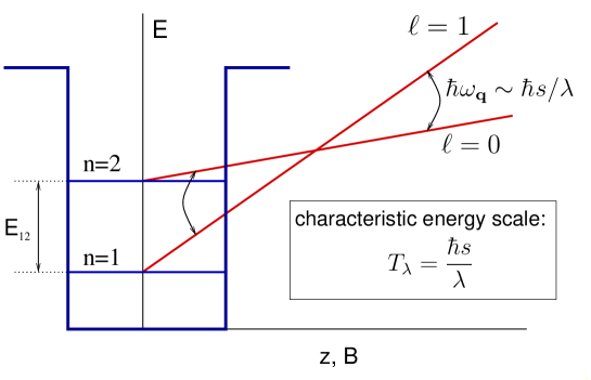
FIG. 1.: A crossing of two Landau levels belonging to different subbands of size quantisation. Phonon transitions are most favorable for phonons with $q\sim 1/\lambda$.

FIG. 2.: S-matrix expantion of the two-particle Green’s function $\Pi(\tau)$. The solid line and the dashed line represent the Green’s functions of the non-perturbed electron and phonon respectively. The wavy line was introduced to account for the Matsubara frequency $i\omega_{n}$ and for the action of the operator $\hat{Q}_{y}$.

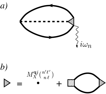
FIG. 3.: Results of graphical summation of the perturbation series expansion. a) A diagram for the exact $\tilde{\Pi}(i\omega_{n})$ expressed in terms of the exact electron Green’s function (bold solid line), the exact phonon Green’s function (bold dashed line), and the total vertex part (shaded triangle). b) A Dyson-type equation for the total vertex part, deducing the evaluation of the total vertex part to the problem of electron-electron interaction via exchange of phonons. The shaded square is the total vertex part for this problem.

FIG. 4.: The first term of the pertubration expansion of the electron self energy.

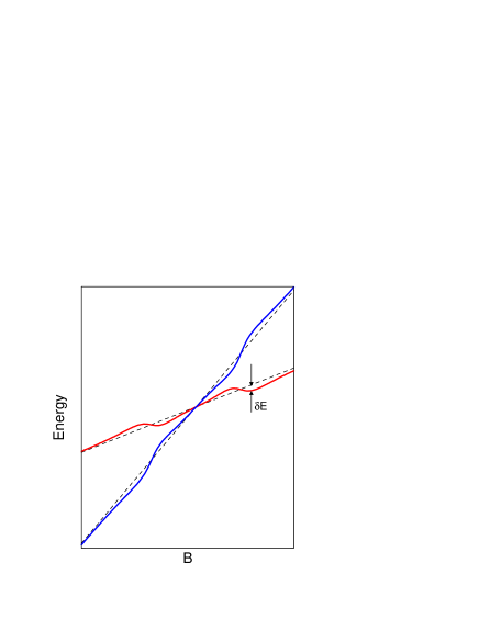
FIG. 5.: Qualitative behaviour of the Landau levels in the vicinity of a level-crossing. The dashed lines represent the non-perturbed Landau levels.

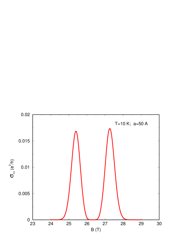
FIG. 6.: The dissipative conductivity as a function of magnetic field in the vicinity of crossing of the Landau levels $\ell=1$ and $\ell=0$ belonging to the first and second size-quantization subbands, respectively. Material parameters are taken as for a GaAs system.

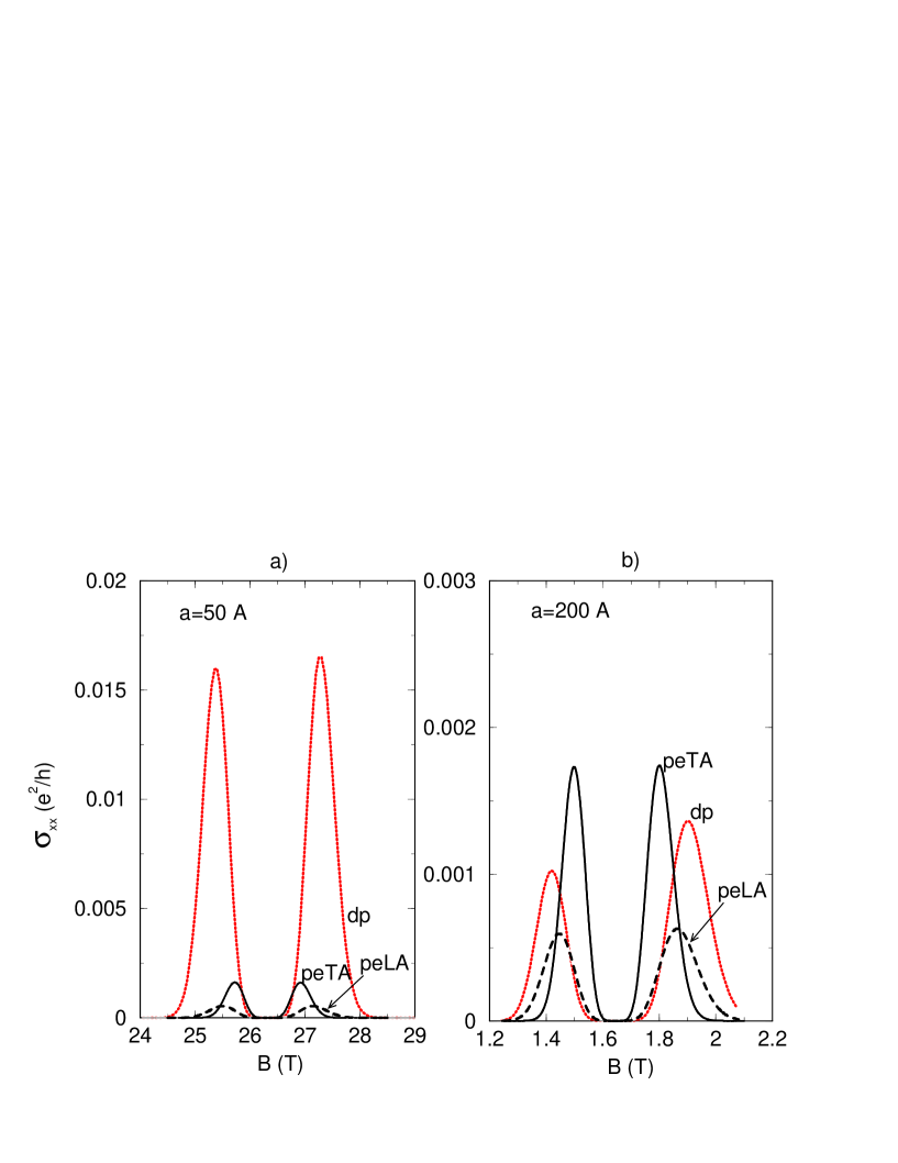
FIG. 7.: A comparison of contributions into $\sigma_{xx}$ from different mechanisms of electron-phonon interaction at two values of the quantum well width $a$. The lines are labeled as follows: the deformation potential mechanism - dp, the piezoelectric longitudinal mechanism - peLA, and the piezoelectric transversal mechanism - peTA.

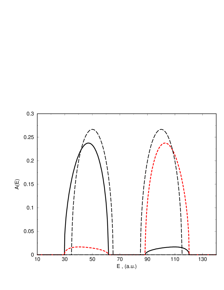
FIG. 8.: Level mixing.

REFERENCES

- [1] M. Sh. Erukhimov, Fiz. Tekh. Poluprovodn. 3, 194 (1969) [Sov. Phys. Semicond. 3, 162 (1969)].
- [2] V. V. Korneev, Fiz. Tverd. Tela (Leningrad) 19, 357 (1977) [Sov. Phys. Solid State 19, 205 (1977)].
- [3] K. A. Benedict, R. K. Hills, and C. J. Mellor, Phys. Rev. B 60, 10 984 (1999).
- [4] K. A. Benedict, J. Phys.: Condens. Matter 3, 1279 (1991).
- [5] G. A. Toombs, F. W. Sheard, D. Neilson, andL. J. Challis, Solid State Commun. 64, 577 (1987).
- [6] V. I. Fal’ko and L. J. Challis, J. Phys.: Condens. Matter 5, 3945 (1993).
- [7] P. A. Maksym, Springer Series in Solid-State Sciences, vol. 101, editor: G. Landwehr (Springer-Verlag Berlin Heidelberg 1992).
- [8] V. M. Apalkov and M. E. Portnoi, cond-mat/0111378; cond-mat/0111377.
- [9] I. M. Lifshitz, Zh. Eksp. Teor. Fiz. 33, 1569 (1960) [Sov. Phys. JETP 11, 1130 (1969)].
- [10] N. N. Ablyazov, M. Yu. Kuchiev, and M. E. Raikh, Phys. Rev. B 44, 8802 (1991).
- [11] D. V. Lang, in Deep Centers in Semiconductors, edited by S. T. Pantelides (Gordon and Breach, New York, 1986), p. 486.
- [12] A. Kastalsky and J. C. M. Hwang, Solid State Commun. 51, 317 (1984).
- [13] I. V. Kukushkin, K. von Klitzing, and K. Ploog, Phys. Rev. B 40, 4179 (1989).
- [14] A. J. Turberfield, S. R. Haynes, P. A. Wright, R. A. Ford, R. G. Clark, J. F. Ryan, J. J. Harris, and C. T. Foxon, Phys. Rev. Lett. 65, 635 (1990).
- [15] A. S. Plaut, K. v. Klitzing, I. V. Kukushkin, and K. Ploog, Proceedings of the 20th International Conference on the Physics of Semiconductors, Vol. 2, [Editors: E. M. Anastassakis, and J. D. Joannopoulos], p. 1529 (1990).
- [16] I. V. Kukushkin, V. B. Timofeev, K. von Klitzing, and K. Ploog, Festkörperprobleme (Advances in Solid State Physics), edited by U. Rössler (Pergamon, Braunschweig, 1988), Vol. 28, p. 21.
- [17] Yu. A. Bychkov, S. V. Iordanski, and G. M. Eliashberg, Pis’ma Zh. Eksp. Teor. Fiz. 34, 496 (1981) [JETP Lett. 34, 473 (1981)].
- [18] J. P. Wolfe, M. R. Hauser, Ann. Physik 4, 99 (1995).
- [19] R. Kubo, J. Phys. Soc. Japan 12, 570 (1957).
- [20] L. D. Landau, E. M. Lifshitz, Quantum Mechanics (Pergamon Press Ltd. 1977).
- [21] R. Kubo, H. Hasegawa, and N. Hashitsume, J. Phys. Soc. Japan 14 56 (1959).
- [22] R. Kubo, S. Miyake, and N. Hashitsume, Solid State Physics edited by F. Seitz and D. Turnbull, Vol. 17, p. 169 (Academic Press, 1965).
- [23] See for example: G. D. Mahan, Many-Particle Physics (Plenum Press, New York, 1981).
- [24] A. Asihara, Statistical Physics (Academic Press 1971); K. Efetov, Supersymmetry in disorder and chaos (Chambridge University Press 1997).
- [25] A. A. Abrikosov, L. P. Gor’kov, and Dzyaloshinskii, Methods of Quantum Field Theory in Statistical Physics, (Pergamon Press 1965).
- [26] Note that . For more information see: V. F. Gantmakher and Y. B. Levinson, Carrier Scattering in Metals and Semiconductors (North-Holland, Amsterdam, 1987).