Gate errors in solid state quantum computer architectures

Abstract

We theoretically consider possible errors in solid state quantum computation due to the interplay of the complex solid state environment and gate imperfections. In particular, we study two examples of gate operations in the opposite ends of the gate speed spectrum, an adiabatic gate operation in electron-spin-based quantum dot quantum computation and a sudden gate operation in Cooper pair box superconducting quantum computation. We evaluate quantitatively the non-adiabatic operation of a two-qubit gate in a two-electron double quantum dot. We also analyze the non-sudden pulse gate in a Cooper-pair-box-based quantum computer model. In both cases our numerical results show strong influences of the higher excited states of the system on the gate operation, clearly demonstrating the importance of a detailed understanding of the relevant Hilbert space structure on the quantum computer operations.

The rapid progress of quantum information theory has prompted intense interest in developing appropriate hardwares for quantum computation and communication [1]. Since quantum coherence needs to be maintained for a quantum computer (QC) to maximize its capability, it has to satisfy stringent requirements [2]. One requirement is that a QC should have a well-delineated Hilbert space, while another requirement is that the quantum bits (qubit) should have long coherence time (i.e. slow decoherence). Indeed, decoherence can be loosely defined as irreversibly losing information from the operational Hilbert space into the environment, which is the rest of the universe from the perspective of a QC system. Furthermore, the requirement of slow decoherence needs to be satisfied not only when the qubits are standing alone, but also when the qubits are interacting with each other or are manipulated externally for single or multi-qubit operations.

Many physical systems with suitable two-level quantum dynamics have been suggested as possible candidates for qubits in a variety of QC architectures. The proposals based on solid state systems, such as the ones based on electron spins [3, 4, 5, 6], nuclear spins [7, 8], and superconductors [9, 10], are particularly attractive because of their potential for scalability. However, solid state structures also present complex environments and fast decoherence rates [12]. For example, for electron spins trapped in quantum dots (QD), their environment includes the underlying crystal lattice in terms of phonons, surrounding electron and nuclear spins, impurities and interfaces, unintentionally trapped charges, and many other defects invariably present in a solid state environment. Even the orbital degrees of freedom of the electron spin qubits themselves are part of the environment. In the case of QC based on Cooper pair boxes (CPB), the environment includes defects in the Josephson junctions, quasiparticles, electromagnetic couplings, etc. From the perspective of qubit Hilbert space, the complex environment in a solid means considerable difficulty in identifying the boundary. The fuzziness in the qubit environment also implies that a gate operation that is not optimized (a gate error) can cause not only incomplete rotations in the qubit Hilbert space, but also leakage into the environment. Thus, to ensure successful operation of a QC, we have to clearly understand how each of the environmental elements affects the QC coherent evolution, and clarify the effects of imperfections in gate operations. In this paper we will investigate specifically the latter effect.

Some of the QC proposals satisfy the requirement for precise coherent manipulation by employing resonant means such as resonant Rabi oscillation and resonant Raman scattering [13]. However, in most solid state QC schemes, non-resonant operations [3, 7, 9] are crucial components of the QC operation. In the spin-based schemes, adiabatic switching of exchange interaction is a cornerstone of the two-qubit operations, while in the CPB-based scheme, sudden switching of a voltage bias has been proposed and used to perform single-qubit operations. Here we study whether QC system integrity can be faithfully maintained if the exchange interaction switching is not adiabatic in the QD case, or the voltage pulse is not switched on suddenly in the CPB case. More specifically, we would like to explore the gate operation threshold when leakage due to non-resonant operations is sufficiently small so that quantum error correction codes can be effectively applied. A quantitative and qualitative theoretical investigation of this issue is clearly important in understanding the feasibility of proposed QC architecture.

Let us first examine the spin-based quantum dot quantum computer (QDQC) in GaAs. Here effects of non-adiabaticity in the single-qubit operations should be relatively weak because bulk spin-orbit coupling at the bottom of GaAs conduction band is small. If the Rashba spin-orbit coupling can also be minimized for the GaAs heterostructure, the overall spin-orbit coupling should be very small so that applied magnetic field pulses will not be able to mix electron spin and orbital states. For two-qubit operations, the adiabatic condition can be satisfied more easily with larger single electron excitation energy and larger on-site Coulomb interaction, which are both consequences of small QDs. However, the size of a gated quantum dot is limited from below by gate and device dimensions. Thus we would like to quantitatively assess the adiabatic condition for two-qubit operations in a double dot of realistic dimensions. In particular, we would like to determine the minimum duration of two-qubit operations constrained by adiabaticity and the quantum error correction threshold.

To deal with a system described by a slowly-time-dependent Hamiltonian, the adiabatic approximation can be employed, in which the state of a quantum system at time $t$ can be expanded on the instantaneous eigenstates at that time [15]: $\psi(t)=\sum_{i}c_{i}(t)u_{i}(t)$ and $H(t)u_{i}(t)=E_{i}(t)u_{i}(t)$. Substituting these two equations into the time-dependent Schrödinger equation, the time evolution of the coefficients $c_{i}(t)$ can be obtained:

$$\frac{\partial c_{k}(t)}{\partial t}=\sum_{i\neq k}^{N}\frac{c_{i}(t)}{E_{k}(t)-E_{i}(t)}\langle k|\frac{\partial H(t)}{\partial t}|i\rangle\,\exp\left\{\frac{1}{i\hbar}\int_{-\infty}^{t}(E_{i}(\tau)-E_{k}(\tau))d\tau\right\}\,.$$ (1)

In our calculation for the exchange gate of a QDQC, we consider a two-electron double quantum dot [4]. The basis states $u_{i}$ are the two-electron eigenstates of the double dot. The explicit time-dependence is in the inter-dot barrier height. In other words, our complete confinement potential is given by $V({\bf r},t)=V_{L}({\bf r})+V_{R}({\bf r})+V_{b}({\bf r},t)$, where $V_{L}({\bf r})$ and $V_{R}({\bf r})$ are the fixed single quantum dot confinement potentials, while $V_{b}({\bf r},t)$ is a Gaussian barrier potential that takes the form $V_{b}({\bf r},t)=\left[V_{max}-(V_{max}-V_{min})e^{-\left(\frac{t}{\tau}\right)^{2}}\right]e^{-\left(x^{2}/l_{x}^{2}+y^{2}/l_{y}^{2}\right)}$. Here $V_{max}$ and $V_{min}$ are the highest and lowest barriers respectively, $l_{x}$ and $l_{y}$ defines the width and thickness of the potential barrier between the two QDs located at $x=\pm a$ on the $y$ axis, and $\tau$ is the half width of the Gaussian temporal variation of the barrier height. We have chosen to use Gaussian lineshapes for the confinements, barrier, and time dependence without loss of generality. Indeed, as we point out below, non-Gaussian-shaped pulses might produce more favorable conditions for the operation of two-qubit gates. Now the matrix elements of the time derivative of the Hamiltonian can be expressed completely in terms of the potential barrier matrix elements: $\langle i|\frac{\partial H(t)}{\partial t}|j\rangle=\langle i|\frac{\partial V_{b}(t)}{\partial t}|j\rangle=\left(\langle i|V_{max}|j\rangle-\langle i|V_{b}(t)|j\rangle\right)\frac{2t}{\tau^{2}}\,.$ The wavefunction coefficients can then be calculated by plugging these matrix elements into Eq. (1).

We perform a numerical calculation for the evolution of a two-electron double dot using Eq. (1). Initially the system is entirely in the ground singlet state. In other words, $c_{i}=\delta_{i0}$ for all $i$. The variation of the potential barrier will not lead to singlet-triplet coupling. Both types of states have about the same excitation gap (smaller of the single particle excitation energy and the on-site Coulomb charging energy) and similar energy spectra, and the exchange coupling does not lead to transitions between singlet and triplet states, so that a pure singlet initial state should give a reliable description of adiabaticity for a general case. By varying the half width $\tau$ of the barrier variation time, we quantitatively evaluate the change in the ground singlet state population, thus obtaining a lower limit to the gate operating time using the criterion of quantum error correction code threshold. In the direct integration of Eq. (1), spectrum information such as the barrier matrix elements and eigen-energies are needed. We do not attempt to calculate the state spectrum at all barrier heights, as it would have made the whole computation intractable. Instead, we perform the spectrum calculation at a series of potential barrier heights (at 10 points which correspond to 19 points on the Gaussian temporal profile of the barrier variation), then obtain the rest of the information through interpolation. The energy spectra we use are for a double dot with Gaussian confinements of 30 nm radii and 40 nm inter-dot distance [4]. The energy barrier height $V_{b}$ ranges between 14 meV and 35 meV, corresponding to exchange splitting of 280 $\mu$eV to 3.3 $\mu$eV.

The result of our calculation is plotted in Fig. 1(a). The leakage (y-axis) is defined as $1-|c_{0}|^{2}$ which is zero before the gate is applied, and should be zero if the gate is perfectly adiabatic. The curve has several interesting features. At short gating times the leakage decreases quite fast, with the straight line in Fig. 1 giving an indication of the speed of this decrease. This decrease rate slows down as the gating time increases. At very long time, adiabatic approximation should be asymptotically exact, so that the $k$th excited state occupation takes the form

$$|a_{k}|^{2}=\frac{4\sin^{2}\omega_{k0}t/2}{\hbar^{2}\omega_{k0}^{4}}\left|\langle k|\frac{\partial V_{b}}{\partial t}|0\rangle\right|^{2}\,.$$ (2)

The magnitude of the probability amplitude $a_{k}$ is in the order of the ratio between the change in the Hamiltonian in one Bohr period $2\pi/\omega_{k0}$ and the energy difference $\hbar\omega_{k0}$. Thus the leakage should be proportional to $1/T^{2}$ at large $T$ if we qualitatively represent $\partial H/\partial t$ by $\Delta H/T$ where $T$ characterizes the total gating time.

The leakage we obtained oscillates quite rapidly with the gating time. This oscillation is due to the phase factors $\exp\left\{\frac{i}{\hbar}\int_{-\infty}^{t}\Delta E_{ki}(\tau)d\tau\right\}$ for all the levels involved. As the gating time is varied, the contribution to the leakage from different higher levels changes rapidly, leading to the fast oscillations.

Figure 1(a) demonstrates that for gating time ($\sim 2\tau$) longer than 30 ps, leakage in our double dot system should be sufficiently small ($\lesssim 10^{-6}$) so that the currently available quantum error correction schemes would be effective. On the other hand, an exchange splitting of 0.1 meV corresponds to about 20 ps gating time for a swap gate [3] (with rectangular pulse) at the shortest. Therefore, adiabatic condition does not place an extra burden on the operation of the two-qubit gates such as a swap. There is in general no need to significantly increase the gating time in order to accommodate the adiabatic requirement.

Figure 1(b) shows the energy splittings between the ground singlet and the 1st and 2nd excited singlet states. A finite gap between the ground and excited states exists for all barrier heights, thus guaranteeing the relatively easy satisfaction of adiabatic condition in this configuration. The anti-crossing in this figure shows a competition between S-P hybrid states (one electron in the single dot S states while the other in the single dot P states [4]) and double occupied states (both electrons are in the S state of the same dot) in the double dot. Essentially, this competition indicates the relative importance of single particle excitation (S-P transition) and on-site Coulomb interaction. At high barrier height, the S-P hybrid state has lower energy than the double occupied state, while at lower barrier the 1st excited singlet state is a mixture of the double occupied state and the S-P hybrid state. As the inter-dot barrier is lowered, the two electrons can tunnel between the two dots more easily, thus reducing the effect of on-site Coulomb repulsion.

The duration of the gate voltage pulse that changes the barrier height between two neighboring QDs is not the only parameter that determines whether adiabaticity is satisfied. Pulse shape tailoring is extensively used in optical control experiments [16], and is presumably applicable in the control of interdot barrier. Our choice of a Gaussian pulse shape is by no means optimal. Therefore, the result shown here provides an upper limit to the adiabatic condition for the adopted parameters in the spin-based QDQC architecture.

One condition for the adiabatic approximation to be valid is that the system has no level crossing during the evolution. In the double QD system, there should be no orbital degeneracy as we lower the inter-dot barrier. The situation bears some similarity to the transition from a hydrogen molecule to a helium atom, although in the operation of a QDQC we would never push the two QDs so close and the barrier so low that the two-electron double dot becomes a two-electron single dot. Here the state spectrum essentially maintains the same structure throughout the gate operation. It would, however, be interesting to explore the state spectrum as the double dot is squeezed towards a single QD, and study whether degeneracy might play a role during such evolution. After all, in a QDQC, QDs are used to label the qubits; while in a two-electron QD, labeling is impossible as the two electrons are indistinguishable.

Let us now turn our attention to the Cooper pair box quantum computer (CPBQC) model. The Hamiltonian of a CPB can be written on the basis of charge number states of the box:

$$H = 4E_{C}(\hat{n}-n_{g})^{2}-E_{J}\cos\hat{\phi}$$ (3)

$$= \sum_{n}\left[4E_{C}(n-n_{g})^{2}|n\rangle\langle n|-\frac{E_{J}}{2}(|n\rangle\langle n+1|+|n+1\rangle\langle n|)\right]\,,$$ (4)

where $E_{C}$ is the charging energy of a Cooper pair box (CPB), $E_{J}$ is the Josephson coupling between the CPB and an external superconducting lead, $n_{g}$ represents the applied voltage on the CPB in terms of an effective charge number, and $n$ refers to the number of Cooper pairs in the box. The stationary solutions of a CPB form energy bands. The two levels for a CPB qubit are the lowest two energy levels at $n_{g}=1/2$, where the eigenstates are approximately $|\!\downarrow\rangle=(|0\rangle+|1\rangle)/\sqrt{2}$ and $|\!\uparrow\rangle=(|0\rangle-|1\rangle)/\sqrt{2}$ with a splitting of about $E_{J}$.

Most theoretical studies of CPBQC employ a two-level description of the system [9]. However, as we have learned [4, 5] in the case of QDQC above, higher excited states can play an important role in the dynamics of a qubit, especially when it is subjected to non-resonant operations. One particular operation for CPBQC is the sudden pulse gate to shift $n_{g}$, thus bringing a system from a pure ground state ($|0\rangle$ at, e.g. $n_{g}=1/4$) to a coherent superpositioned state ($(|\!\uparrow\rangle+|\!\downarrow\rangle)/\sqrt{2}$ at $n_{g}=1/2$). However, such a simple description of the pulse gate is only valid when $E_{J}/E_{C}\rightarrow 0$. Since $E_{J}$ determines the gate speed of a CPBQC, such a condition is not practical for a realistic QC. Below we explore the situation when $E_{J}$ is not vanishingly small, and study how the pulse gate operation will be affected.

Before considering the pulse gate, we first study the state compositions of a CPB in order to find the limit of a two-level model and show some analytical results in Table I (For these expressions, we include only the lowest excited states). As is shown in Table I, no matter which $n_{g}$ value we choose, there are always unwanted states that mix into the composition of the eigenstates with weights proportional to $r=E_{J}/E_{C}$. Such mixtures will affect the dynamics of the system. For example, if we prepare a CPB in the ground state $\psi_{0}$ at $n_{g}=1/4$ and apply a sudden pulse gate to shift $n_{g}$ up to $1/2$, the state right after the shift will not be $(|\!\uparrow\rangle+|\!\downarrow\rangle)/\sqrt{2}$, but $\approx(|\!\uparrow\rangle+|\!\downarrow\rangle)/\sqrt{2}+\frac{r}{4}(|\!\uparrow\rangle-|\!\downarrow\rangle)/\sqrt{2}$. Thus, finite $r$ will lead to errors in the pulse gate to the first order of $r$.

In real experiments, the pulse gate always has finite rise/fall times (non-sudden). In Ref. [11], the pulse rise time is in the range of 30 to 40 ps. Such gradual rise and fall of the pulse gate inevitably lead to more errors, which have been considered in the context of two-level systems [17, 18]. Here we calculate the fidelity of the pulse gate taking into account the finite rise/fall time, the higher excited states, and the complete composition of all the eigenstates. The eigenstates are numerically obtained (instead of perturbatively [19]) on the basis of 21 charge number states ($|-10\rangle$, $\cdots|0\rangle$, $|1\rangle$, $\cdots|10\rangle$). We prepare the initial state as the ground state $\psi_{0}$ near $n_{g}=1/4$, then let the CPB evolve under Hamiltonian (4). The pulse gate represented by $n_{g}$ is turned on with a lineshape ranging from linear to quintic power of time during the rise and fall: $n_{g}(t)=n_{g}(0)+\left(\frac{2t}{t_{r}}\right)^{m}(n_{g}(t_{r})-n_{g}(0))/2$ for $t\in[0,t_{r}/2]$ and $n_{g}(t)=n_{g}(t_{r})-\left[\frac{2(t_{r}-t)}{t_{r}}\right]^{m}(n_{g}(t_{r})-n_{g}(0))/2$ for $t\in[t_{r}/2,t_{r}]$, where $t_{r}$ is the pulse rise/fall time and the pulse is switched on from $0$ to $t_{r}$. For system parameters, we choose the values used in Ref. [11], with $E_{C}=117$ $\mu$eV, $E_{J}=51.8$ $\mu$eV, $n_{g}(0)=0.255$, and $n_{g}(t_{r})=0.5$.

In Fig. 2 we plot the state fidelity as a function of rise time. Here the state fidelity is defined as the maximum probability for the CPB to be in the first excited state after the pulse gate when $n_{g}$ returns to $0.255$. Figure 2 illustrates two important points. First of all, the fidelity of the pulse gate decreases oscillatorily instead of monotonously as the pulse rise time increases. The oscillations (with periods of 30 to 40 ps) in the curves represent the coherent evolution of the CPB during the rise/fall of the pulse voltage: at $n_{g}=1/4$, the dominant energy scale is $2E_{C}\approx 234\ \mu$eV with a corresponding period of 17 ps, while at $n_{g}=1/2$ the dominant energy scale is $E_{J}=51.8\ \mu$eV with a corresponding oscillation period of 76 ps. The observed oscillation period is essentially an average of these two limits. Secondly, including higher excited states is important in correctly evaluating the fidelity dependence on pulse rise time, as a comparison of the two panels of Fig. 2 clearly demonstrates, especially for higher power of time-dependence. The real pulse shape may not be the same as any of the power law time-dependence we consider here, but the disagreement between the two panels in Fig. 2 clearly shows again the necessity of taking excited states into consideration when evaluating non-resonant gates such the pulse gate here.

Our current study is in essence a quantitative delineation of the Hilbert space for a QDQC (CPBQC) during a two-qubit (single-qubit) operation. Such a study is necessary for other proposed QC schemes as well in order to select the optimal operating regime, eliminate possible errors, and enhance signal to noise ratios in experiments. We have restricted ourselves to $T=0$ in our calculations, but our results remain valid at finite (low) temperatures as long as substantial thermal occupation of higher excited levels does not occur in the system.

We thank David DiVincenzo and Belita Koiller for useful discussions, and ARDA and LPS for financial support.

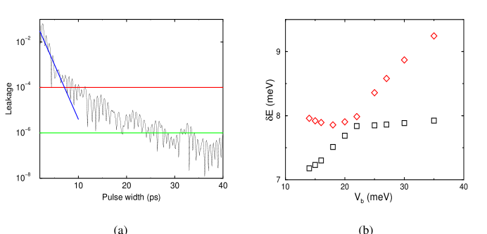
FIG. 1.: In (a) we plot the state leakage as a function of the pulse width $2\tau$ of the exchange gate. The two-electron state is initially prepared in the ground singlet state. The two horizontal lines represents the commonly used threshold for quantum error correction. The fitted line at the small pulse-width indicates the initial rapid decrease in the error rate (leakage) as the pulse becomes wider (or the gate operation becomes slower). In (b) we plot the energy splitting between the ground singlet state and the first and second excited singlet states as functions of inter-dot barrier height. The presence of this gap for all barrier heights is important in making the adiabatic condition easier to satisfy.

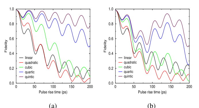
FIG. 2.: State fidelity as a function of the finite rise/fall time of a pulse gate in a single Cooper pair box. The fidelity here is defined as the maximum probability of the CPB in the first excited state after the application of a pulse gate with the state starting from the ground state (represented by $n_{g}$ goes from 0.255 to 0.5, then back to 0.255 after a period of time $\tau_{p}$). In panel (a), the CPB is treated as a two-level system (on the basis of $|0\rangle$ and $|1\rangle$), while in panel (b) the CPB is treated as a multi-level system (on the basis of $|-10\rangle,\cdots,|0\rangle,|1\rangle,\cdots,|10\rangle$).The five curves in each panel represent the different lineshapes of the rise/fall of the pulse ranging from linear to quintic, as described in the text.

TABLE I.: Eigenstates and energies of a Cooper pair box.

$n_{g}$	low energy eigenstates	$b/a$ ($r=E_{J}/E_{C}$)	eigenenergies
0	$\psi_{0}=a|0\rangle+b(|1\rangle+|-1\rangle)$	$r/8$	-$\frac{E_{J}^{2}}{8E_{C}}$
	$\psi_{1}=(|1\rangle-|-1\rangle)/\sqrt{2}$	—	$4E_{C}$
	$\psi_{1}=a(|1\rangle-|-1\rangle)-b|0\rangle$	r/4	$4E_{C}+\frac{E_{J}^{2}}{8E_{C}}$
$\approx 1/4$	$\psi_{0}=a|0\rangle+b[\frac{|-1\rangle}{1+2n_{g}}+\frac{|1\rangle}{1-2n_{g}}]$	$r/8$	$4E_{C}n_{g}^{2}-\frac{E_{J}^{2}}{8E_{C}(1-4n_{g}^{2})}$
	$\psi_{1}=a|1\rangle+b[\frac{|2\rangle}{3-2n_{g}}+\frac{|0\rangle}{1-2n_{g}}]$	$r/8$	$4E_{C}(1-n_{g}^{2})-\frac{E_{J}^{2}}{8E_{C}(3-2n_{g}^{2})(1-2n_{g}^{2})}$
$1/2$	$\psi_{0}=a(|0\rangle+|1\rangle)+b(|-1\rangle+|2\rangle)$	$r/18$	$E_{C}-E_{J}/2-\frac{E_{J}^{2}}{32E_{C}}$
	$\psi_{1}=a(|0\rangle-|1\rangle)+b(|-1\rangle-|2\rangle)$	$r/18$	$E_{C}+E_{J}/2-\frac{E_{J}^{2}}{32E_{C}}$

REFERENCES

- [1] A. Steane, Rep. Prog. Phys. 61, 117 (1998); C.H. Bennett and D.P. DiVincenzo, Nature 404, 247 (2000).
- [2] D.P. DiVincenzo, Fortschr. Phys. 48, 771-783 (2000).
- [3] D. Loss and D.P. DiVincenzo, Phys. Rev. A 57, 120 (1998).
- [4] X. Hu and S. Das Sarma, Phys. Rev. A 61, 2301 (2000).
- [5] X. Hu and S. Das Sarma, Phys. Rev. A 64, 042312 (2001).
- [6] R. Vrijen et al., Phys. Rev. A 62, 012306 (2000).
- [7] B.E. Kane, Nature 393, 133 (1998); Fortschr. Phys. 48, 1023 (2000).
- [8] V. Privman, I.D. Vagner, and G. Kventsel, Phys. Lett. A 239, 141 (1998); D. Mozyrsky, V. Privman, and M.L. Glasser, Phys. Rev. Lett. 28, 5112 (2001).
- [9] A. Shnirman, G. Schön, and Z. Hermon, Phys. Rev. Lett. 79, 2371 (1997); Y. Makhlin, G. Schon, and A. Shnirman, Rev. Mod. Phys. 73, 357 (2001).
- [10] D.V. Averin, Solid State Comm. 105, 659 (1998).
- [11] Y. Nakamura, Y.A. Pashkin, and J.S. Tsai, Nature 398, 786 (1999).
- [12] X. Hu, R. de Sousa, and S. Das Sarma, LANL preprint cond-mat/0108339.
- [13] J.I. Cirac, P. Zoller, Phys. Rev. Lett. 74, 4091 (1995); C. Monroe, D.M. Meekhof, B.E. King, W.M. Itano, and D.J. Wineland, Phys. Rev. Lett. 75, 4714 (1995).
- [14] We have shown that under certain conditions multielectron QD can also be used as qubit for a QDQC [5]. The considerations regarding adiabatic condition would be similar in that architecture, while here we will focus on single-electron QDs.
- [15] L.I. Schiff, Quantum Mechanics (McGraw-Hill, New York, 1968).
- [16] I.P. Christov, R. Bartels, H.C. Kapteyn, and M.M. Murnane, Phys. Rev. Lett. 86 5458 (2001); C. Rangan and P. H. Bucksbaum, Phys. Rev. A 64, 033417 (2001).
- [17] M-S Choi, R. Fazio, J. Siewert, and C. Bruder, Europhys. Lett. 53, 251 (2001).
- [18] S. Oh, quant-ph/0201068.
- [19] X. Wang, M. Keiji, H. Fan, and Y. Nakamura, quant-ph/0112026.