SUNY-NTG-2002/06

Critical statistics for non-Hermitian matrices

A.M. García-García¹, S.M. Nishigaki² and J.J.M. Verbaarschot¹

¹Department of Physics and Astronomy, SUNY, Stony Brook, New York 11794-3800

²Department of Physics, University of Connecticut, Storrs, Connecticut 06269-3046

Abstract

We introduce a generalized ensemble of nonhermitian matrices interpolating between the Gaussian Unitary Ensemble, the Ginibre ensemble and the Poisson ensemble. The joint eigenvalue distribution of this model is obtained by means of an extension of the Itzykson-Zuber formula to general complex matrices. Its correlation functions are studied both in the case of weak nonhermiticity and in the case of strong nonhermiticity. In the weak nonhermiticity limit we show that the spectral correlations in the bulk of the spectrum display critical statistics: the asymptotic linear behavior of the number variance is already approached for energy differences of the order of the eigenvalue spacing. To lowest order, its slope does not depend on the degree of nonhermiticity. Close the edge, the spectral correlations are similar to the Hermitian case. In the strong nonhermiticity limit the crossover behavior from the Ginibre ensemble to the Poisson ensemble first appears close to the surface of the spectrum. Our model may be relevant for the description of the spectral correlations of an open disordered system close to an Anderson transition.

PACS: 11.30.Rd, 12.39.Fe, 12.38.Lg, 71.30.+h
Keywords: Random Matrices; Spectral Correlations; Ginibre Model; Critical Statistics; Fermi-Gas Method.

1 Introduction

Nonhermitian Random Matrix Models were first introduced by Ginibre in 1965 [1]. His motivation was to describe the statistical properties of nuclear resonances with a finite width in complete analogy with the description of the position of resonances by means Hermitian Random Matrix Ensembles as introduced by Wigner and Dyson [2]. Since then, eigenvalues of nonhermitian operators occurring in many different fields have been analyzed in terms of nonhermitian random matrix models, usually with additional ingredients. We mention several examples. The statistical properties of the poles of $S$-matrices have been analyzed in great detail in [3, 4, 5]. In QCD, the Euclidean Dirac operator in QCD at nonzero chemical potential (which can be interpreted as an imaginary vector potential), is nonhermitian resulting in the failure of the quenched approximation [6]. Both this failure and the generic properties of the complex Dirac spectrum have been explained fully in terms of a nonhermitian Random Matrix Model with the global symmetries of QCD [7, 8, 10, 9, 11]. Recently, a delocalization transition was found in a one-dimensional lattice model with an imaginary vector potential [12, 13]. Statistical correlations predicted by the Ginibre ensemble have been found dissipative quantum maps [14, 15, 16]. Eigenvalue spacings of the Floquet matrix of a Fokker Planck equation have been described in terms of Ginibre statistics [17]. In [18, 19] an ensemble of asymmetric real matrices, closely related to the Ginibre ensemble, was utilized to model the dynamics of a neural network.

Among more mathematically oriented works we mention the exact calculation of the correlation functions of an ensemble of normal random matrices with an arbitrary polynomial probability potential [20, 21]. Nonhermitian ensembles have been analyzed in terms of associated hermitian ensembles [22, 23]. Correlations of eigenfunctions have been studied in the Ginibre ensemble [24]. Another intriguing application is the description of an analytic curve by the boundary of the support of the complex spectrum of a nonhermitian Random Matrix Theory [25, 26]. Finally, we point out that there are interesting relations between the eigenvalues of complex matrices and the positions of particles in certain two dimensional physical systems [28, 27, 29]. For example, the Ginibre model is equivalent to a Coulomb problem in two dimensions [1].

Based on the magnitude of the imaginary part of the eigenvalues we distinguish two types of nonhermiticity: weak nonhermiticity and strong nonhermiticity. Weak nonhermiticity is the limit of large matrices when the imaginary part of the eigenvalues remains comparable with the mean separation of eigenvalues along the real axis. This limit was identified in [30, 31, 32], but was used earlier in the statistical theory of $S$-matrices [3]. Strong nonhermiticity refers to cases for which the real and imaginary parts of the eigenvalues remain of the same order of magnitude in the thermodynamic limit. In this article we consider both types of nonhermiticity.

An important concept in the understanding of disordered systems is the Thouless energy. We will define this energy scale as the energy difference below which the eigenvalues are correlated according to Random Matrix Theory. In diffusive disordered systems, in the thermodynamic limit, both the eigenvalue spacing and the Thouless energy approach zero whereas the number of eigenvalues in between them approaches infinity. In this article we will consider critical statistics [33, 34, 35, 36] which refers to the case that the ratio of the Thouless energy and the eigenvalue spacing remains finite in the thermodynamic limit. A Hermitian Random Matrix model for critical statistics was proposed in [37]. In that model the correlations of the eigenvalues decay exponentially beyond a Thouless energy resulting in an asymptotically linear behavior of the number variance with slope (level compressibility) less than one. In this article we generalize this model to complex eigenvalues and analyze its properties. In the Ginibre model the two-point correlation function of eigenvalues in the bulk of the spectrum drops off exponentially on the scale of the distance between the eigenvalues. It is therefore no surprise that we will find the same bulk correlations in such generalized Ginibre model. However, we find nontrivial long range surface correlations, characteristic of a two-dimensional Coulomb liquid. In the case of weak nonhermiticity we expect to find critical statistics similar to the Hermitian model. The analysis of this case is the main objective of this article.

Critical statistics is associated with the multifractal behavior of the eigenfunctions [36, 38, 39]. The critical Hermitian model introduced in [37] has the unitary invariance of the Gaussian Unitary Ensemble with eigenvectors that are distributed according to the measure of the unitary group. This is no contradiction: multifractality of wave functions occurs in a specific basis in which disorder competes with a hopping term. Indeed, in [40, 41] it was found that the fractal dimension of the wave function determines the asymptotic slope of the number variance.

Among others, critical statistics have been utilized to describe the spectral correlations of disordered system at the Anderson transition in three dimensions [33, 42], two dimensional Dirac fermions in a random potential [43], quantum Hall transition [44] and QCD Dirac operator in a liquid of instantons [45, 46]. The scope of universality of critical statistics is still under debate.

Our Random Matrix Model is introduced in section 2. The case or strong nonhermiticity and weak nonhermiticity are analyzed in sections 3 and 4, respectively. Among others we derive a closed expression for the two-point correlation function in both limits. Results for the number variance are discussed in section 5 and concluding remarks are macritical statistics is still under debate.de in section 6.

2 Introduction of the model

Recently, a Hermitian random matrix model for critical statistics was introduced by Moshe, Neuberger and Shapiro [37]. This model, which interpolates between Wigner-Dyson statistics and Poisson statistics, is defined by the joint eigenvalue probability distribution

$$P(H)dH=dH\int dU{\rm e}^{-(1+b){\rm Tr}\,H^{2}+b{\rm Tr}\,UHU^{\dagger}H^{\dagger}},$$ (1)

where $H$ is a Hermitian $n\times n$ matrix. The integral is over the unitary group with invariant measure denoted by $dU$. Critical statistics [36] is obtained in the thermodynamic limit with $b$ scaling as $b=h^{2}n^{2}$ at fixed $h$ . In that case, the two-point correlation function decays exponentially at large distances and the number variance has an asymptotic linear behavior with slope less than one. In the thermodynamic limit, Wigner-Dyson statistics is obtained for a weaker $n$-dependence of $b$, and Poisson statistics is found for a stronger $n$-dependence of $b$.

In this article we are interested in ensembles of nonhermitian random matrices. The study of random matrices with no restrictions imposed was initiated by the classical work of Ginibre [1]. He found closed expressions for the two-point correlation function of the eigenvalues of a Gaussian ensemble of random matrices with complex entries.

An ensemble that interpolates between the Ginibre ensemble and the Wigner-Dyson ensemble of Hermitian matrices was introduced in [30, 31]

$$P(C)dC\sim dC\,{\rm e}^{-\frac{1}{1-\tau^{2}}{\rm Tr}C^{\dagger}C+\frac{\tau}{2(1-\tau^{2})}{\rm Tr}\,(C^{2}+(C^{\dagger})^{2})}.$$ (2)

Here, $C$ is an arbitrary $n\times n$ complex matrix with integration measure given by the product of the real and imaginary parts of the differentials of the matrix elements of $C$. For $\tau=0$ this model reduces to the Ginibre ensemble whereas for $\tau=1$ ($-1$) it reduces to a Gaussian ensemble of (anti-)Hermitian matrices. The eigenvalues of this ensemble are scattered inside an ellipse with eccentricity given by $2\sqrt{\tau}/(1+\tau)$.

The joint eigenvalue distribution can be obtained by using two alternative decompositions

$$C=UTU^{\dagger}\qquad{\rm and}\qquad C=V\Lambda V^{-1},$$ (3)

where $U$ is a unitary matrix, $V$ is a similarity transformation, $T$ a upper triangular matrix and $\Lambda$ a diagonal matrix. The diagonal matrix elements of $T$ coincide with the complex eigenvalues $\Lambda_{kk}=z_{k}$. The invariant measure factorizes as [2]

$$dC\sim dUdT\Delta(\{\Lambda_{kk}\})\Delta(\{\Lambda^{*}_{kk}\})$$ (4)

with the Vandermonde determinant defined by

$$\Delta(\{z_{k}\})=\prod_{k<l}^{n}(z_{k}-z_{l}).$$ (5)

Since the Gaussian integral over the off-diagonal matrix elements of $T$ factorizes it can be performed trivially. The integral over $U$ is equal to the group volume. The joint probability distribution of the eigenvalues is thus given by

$$P(\Lambda)d\Lambda\sim d\Lambda\,|\Delta(\Lambda)|^{2}\,{\rm e}^{-\frac{1}{1-\tau^{2}}\sum_{i=0}^{n}[|z_{i}|^{2}-\frac{\tau}{2}(z_{i}^{2}+(z_{i}^{*})^{2})]}.$$ (6)

This model has been analyzed in two domains: weak nonhermiticity and strong nonhermiticity. In the first case the thermodynamic limit is taken at fixed $n(1-\tau)$, whereas in the case of strong nonhermiticity $-1<\tau<1$ remains fixed for $n\to\infty$. The two-point correlation function of this model was derived in [30].

In this article, we analyze a model that interpolates in between the models defined in eqs. (1) and (6). Our random matrix model is defined by

$$P(C)dC\sim dC\,{\rm e}^{-a_{1}{\rm Tr}\,C^{\dagger}C-\frac{a_{2}}{2}{\rm Tr}\,(C^{2}+(C^{\dagger})^{2})}\int dU{\rm e}^{a_{3}{\rm Tr}\,UCU^{\dagger}C^{\dagger}}.$$ (7)

where is $C$ an arbitrary complex $n\times n$ matrix, and $dU$ is the Haar measure of the unitary group ${\rm U}(n)$. In the special case of $C$ being a normal matrix ($[C,C^{\dagger}]=0$), a unitary transformation brings $C$ to a diagonal form and the integral over $U$ is the standard Itzykson-Zuber integral [47] given by

$$\int dU\,{\rm e}^{a_{3}{\rm Tr}\,UCU^{\dagger}C^{\dagger}}=\frac{\det{\rm e}^{a_{3}z_{i}z_{j}^{*}}}{\Delta(\{z_{k}\})\Delta(\{z^{*}_{k}\})},$$ (8)

where the $z_{i}$ are the eigenvalues of $C$. One thus finds the joint eigenvalue distribution

$$P(\{z_{k}\})\sim{\rm e}^{-\sum_{i=n}^{n}\left[a_{1}|z_{i}|^{2}+\frac{a_{2}}{2}(z_{i}^{2}+z_{i}^{*2})\right]}{\rm det}\left[{\rm e}^{a_{3}z_{i}z_{j}^{*}}\right].$$ (9)

In the next paragraph we will show that this result is valid even if $C$ is an arbitrary complex matrix that can be decomposed according to (3).

We start from the triangular decomposition $C=UTU^{\dagger}$. Since $T$ is an upper-triangular matrix, the exponent in the integral over $U$ in (7) is then given by

$${\rm Tr}\,UCU^{\dagger}C^{\dagger}=\sum_{{j\leq k\atop i\leq l}}~{}U_{ij}T_{jk}U_{lk}^{*}T^{*}_{il}.$$ (10)

After performing a trivial ${\rm U}(1)$ integration, the integral over $U$ in (8) is over ${\rm SU}(n)$. The generating function for such integrals is given by

$$\int_{U\in{\rm SU}(n)}\!\!\!\!dU\,{\rm e}^{{\rm Tr}\,(JU^{\dagger}+J^{\dagger}U)}=F(\det J,\det J^{\dagger},\{{\rm Tr}\,(J^{\dagger}J)^{k}\}),$$ (11)

where $J$ is a complex $n\times n$ matrix and the functional form of the r.h.s., with $k$ running over all positive integers, follows from the invariance of the group integral. In the expansion of the exponent (10) all terms have the same number of factors $U$ and $U^{*}$. By differentiating (11) with respect to $J$ and $J^{*}$ at $J=0$, we find that such terms can be only non vanishing if the sum of the indices of $U$ is equal to the sum of the indices of $U^{*}$ (for the terms that enter in the expansion of the determinant the sum of the first indices is equal to to sum of the second indices). We thus find that in the expansion of (10) all terms with off-diagonal elements of $T$ or $T^{\dagger}$ vanish after integration. We conclude that the result (8) for the Itzykson-Zuber integral is also valid for an arbitrary complex matrix $C$ with eigenvalues $z_{k}$.

For convenience, the constants in the joint eigenvalue distribution of (7) will be parameterized as

$$a_{1} = \frac{\lambda}{1-\tau^{2}},$$

$$a_{2} = -\frac{\lambda\tau}{1-\tau^{2}}+\frac{\lambda\alpha^{2}}{\tau(1-\alpha^{2})},$$

$$a_{3} = \frac{\lambda\alpha}{\tau(1-\alpha^{2})}.$$ (12)

After a rescaling of the matrix elements of $C$ by a factor $1/\sqrt{\lambda}$ the joint eigenvalue distribution of the model (7) reduces to

$$P(\Lambda)d\Lambda\sim d\Lambda\,{\rm e}^{-\sum_{i=1}^{n}\left[\frac{1}{1-\tau^{2}}|z_{i}|^{2}-\frac{\tau}{2(1-\tau^{2})}(z_{i}^{2}+z_{i}^{*2})+\frac{\alpha^{2}}{2\tau(1-\alpha^{2})}(z_{i}^{2}+z_{i}^{*2})\right]}{\rm det}\left[{\rm e}^{\frac{\alpha}{\tau(1-\alpha^{2})}z_{i}z_{j}^{*}}\right].$$ (13)

We will analyze this model in two limits. The case when $1-\tau$ remains finite in the thermodynamic limit will be referred to as strong nonhermiticity. In this class of models we will consider the limiting case of zero eccentricity

$$\alpha\to 0,\quad\tau\to 0\quad{\rm with}\quad\frac{\alpha}{\tau}=b\quad\mbox{fixed},$$ (14)

which reduces to the Ginibre model in the limit in which the parameter $b$ is taken to zero. On the other hand, the case of weak nonhermiticity [30] is defined by the limit

$$\tau\to 1,\ n\to\infty,\quad(1-\tau)n=a^{2}\quad\mbox{fixed}.$$ (15)

Finally, let us mention that the wave functions of our model are distributed according to the invariant Haar measure of ${\rm U}(n)$. It could be that for diagonal $U$ in (7) the wave functions show a multifractal behavior, but that this property is obscured by averaging over all $U$ whereas eigenvalue correlations remain unaffected.

3 Strong nonhermiticity

In this section we consider the case of strong nonhermiticity (14). In order to rewrite the Itzykson-Zuber determinant in Eq.(13) in terms of an expectation value of two Slater determinants, we expand the exponential as

$${\rm e}^{bz_{i}z_{j}^{*}} = \sum_{m=0}^{\infty}\frac{b^{m}}{m!}z_{i}^{m}(z_{j}^{*})^{m}.$$ (16)

By a series of elementary manipulations we find

$$\det{\rm e}^{bz_{i}z_{j}^{*}} = \sum_{m_{1}=0}^{\infty}\cdots\sum_{m_{n}=0}^{\infty}\frac{b^{m_{1}+\dots+m_{n}}}{m_{1}!\cdots m_{n}!}\sum_{\pi\in{\rm S}_{n}}(-1)^{\sigma(\pi)}z_{1}^{m_{1}}(z_{\pi(1)}^{*})^{m_{1}}\cdots z_{n}^{m_{n}}(z_{\pi(n)}^{*})^{m_{n}}$$ (17)

$$= \sum_{m_{1}<m_{2}<\cdots<m_{n}}b^{m_{1}+\dots+m_{n}}\det\frac{z_{i}^{m_{j}}}{\sqrt{m_{j}!}}\det\frac{z_{k}^{*m_{l}}}{\sqrt{m_{l}!}}.$$

Including the other factors of the joint probability distribution we thus find

$$P(z)dz\sim\sum_{m_{1}<m_{2}<\cdots<m_{n}}b^{m_{1}+\dots+m_{n}}\det\phi_{m_{j}}(z_{i})\det\phi_{m_{l}}(z_{k}^{*}),$$ (18)

where the normalized wave functions are given by

$$\phi_{k}(z)={\frac{1}{\sqrt{\pi k!}}}z^{k}{\rm e}^{-|z|^{2}/2}$$ (19)

satisfy the orthogonality relation

$$\int d^{2}z\,\phi_{k}^{*}(z)\phi_{l}(z)=\delta_{kl}.$$ (20)

They are the single particle wave functions of the lowest Landau level of a particle with unit mass in a constant magnetic field perpendicular to the plane. The Hamiltonian of this system is given by $(z=x+iy)$

$$H=\frac{1}{2}(i\partial_{x}-y)^{2}+\frac{1}{2}(i\partial_{y}+x)^{2}.$$ (21)

and the corresponding Schrödinger equation reads

$$H\phi_{k}(z)=\phi_{k}(z).$$ (22)

If we write

$$b={\rm e}^{-\beta}$$ (23)

the joint probability distribution is equal to the diagonal element of the $n$-body density matrix of the lowest Landau level fermions at temperature $1/\beta$, with an additional degeneracy-breaking Hamiltonian given by the absolute value of the angular momentum

$$L=iy\partial_{x}-ix\partial_{y},$$ (24)

or equivalently of

$$\tilde{H}=H+2L=\frac{1}{2}(i\partial_{x}+y)^{2}+\frac{1}{2}(i\partial_{y}-x)^{2}.$$ (25)

The average spectral density $\rho_{n}(z)$, which can be interpreted as the one-particle density, is obtained by integrating the joint eigenvalue density over all coordinates except one. By using the orthogonality relations (19) one easily finds

$$\rho_{n}(z)=\frac{1}{Z_{n}}\sum_{m_{1}<m_{2}<\cdots<m_{n}}\sum_{i=1}^{n}{\rm e}^{-\beta(m_{1}+\cdots+m_{n})}\phi_{m_{i}}(z)\phi_{m_{i}}(z^{*}),$$ (26)

or in an occupation number representation

$$\rho_{n}(z)=\frac{1}{Z_{n}}\sum_{n_{1}+n_{2}+\cdots=n}{\rm e}^{-\beta\sum_{p}pn_{p}}\sum_{k=0}^{\infty}n_{k}\phi_{k}(z)\phi_{k}(z^{*}),$$ (27)

where the occupation number $n_{k}$ runs over $\{0,1\}$. The partition function $Z_{n}$ is defined in the usual way

$$Z_{n}=\sum_{n_{1}+n_{2}+\cdots=n}{\rm e}^{-\beta\sum_{p}pn_{p}}.$$ (28)

Such sums can be easily evaluated in the grand canonical ensemble

$$\rho(z) = \frac{1}{Z}\sum_{n}\zeta^{n}{Z_{n}}\rho_{n}(z)$$ (29)

$$= \sum_{k=1}^{n}\frac{\phi_{k}(z)\phi_{k}(z^{*})}{1+\zeta^{-1}{\rm e}^{\beta k}}\equiv\frac{1}{\pi}k(z,z),$$

where we have introduced the prekernel

$$k(z_{1},z_{2})={\rm e}^{-z_{1}z_{2}^{*}}\sum_{k=0}^{\infty}\frac{(z_{1}z_{2}^{*})^{k}}{k!(1+\zeta^{-1}{\rm e}^{\beta k})}.$$ (30)

The fugacity $\zeta$ is determined by the normalization of the one-particle density

$$n=\sum_{k=0}^{\infty}\frac{1}{1+\zeta^{-1}{\rm e}^{\beta k}}.$$ (31)

For $\beta\ll 1$ the sum can be converted into an integral resulting in

$$\zeta={\rm e}^{n\beta}-1.$$ (32)

Similarly, the two-point correlation function is obtained by integrating over all eigenvalues except two. Again by going to the grand canonical ensemble one easily derives that the connected two-point correlation can be factorized in the result for the Ginibre ensemble and the prekernel (30)

$$R_{2}(z_{1},z_{2})=-\frac{1}{\pi^{2}}{\rm e}^{-|z_{1}-z_{2}|^{2}}|k(z_{1},z_{2})|^{2}.$$ (33)

For $\beta\ll 1$ but $n\beta\gg 1$ a partial resummation of the prekernel (30) results in

$$k(z_{1},z_{2})=\sum_{k=0}^{\infty}\frac{\Gamma(k+1,z_{1}z_{2}^{*})}{k!}\frac{\beta}{4\cosh^{2}(\beta(k-n)/2)},$$ (34)

where $\Gamma(k,x)=\int_{x}^{\infty}t^{k-1}{\rm e}^{-t}dt$ is the incomplete $\Gamma$-function. For $\beta\to 0$ it is justified to make the approximation

$$\frac{1}{1+{\rm e}^{\beta(k-n)}}-\frac{1}{1+{\rm e}^{\beta(k+1-n)}}\approx\frac{\beta}{4\cosh^{2}(\beta(k-n)/2)}.$$ (35)

In the remainder of this subsection we will evaluate the prekernel in several limiting situations.

If the distance of $z_{1}$ and $z_{2}$ (both inside the disk of eigenvalues) to the surface of the disk is much larger than $\beta$, the numerator attains its maximum value when the Fermi-Dirac factor is close to unity. In that case the Fermi-Dirac distribution can be replaced by a sharp cutoff and the two-point correlation function is given by

$$R_{2}(z_{1},z_{2})=-\frac{1}{\pi^{2}}{\rm e}^{-|z_{1}-z_{2}|^{2}}.$$ (36)

Inside the disk the average spectral density is $1/\pi$. The unfolded two-point spectral correlation function thus coincides with the Ginibre result.

A more interesting situation arises in case both $z_{1}$ and $z_{2}$ are close to the surface of the disk of eigenvalues. A nontrivial thermodynamic limit of the surface correlations is obtained for

$$\beta \sim \frac{1}{\sqrt{n}},$$

$$|z_{1}z_{2}^{*}| \sim n,$$

$${\rm arg}(z_{1}z_{2}^{*}) \sim \frac{1}{\sqrt{n}}.$$ (37)

Using the asymptotic expansion for the incomplete $\Gamma$-function we find

$$k(z_{1},z_{2}) = \frac{\beta}{\sqrt{\pi}}\sum_{k=0}^{\infty}\frac{{\rm Erfc}((z_{1}z_{2}^{*}-k)/\sqrt{2k})}{4\cosh^{2}(\beta(k-n)/2)}$$ (38)

$$\approx \frac{\beta}{\sqrt{\pi}}\int_{-\infty}^{\infty}dt\frac{{\rm Erfc}((z_{1}z_{2}^{*}-n-t)/\sqrt{2(n+t)})}{4\cosh^{2}(\beta t/2)},$$

where ${\rm Erfc}(x)=\int_{x}^{\infty}{\rm e}^{-t^{2}}dt$. We parameterize the vicinity of the surface of the domain of eigenvalues as

$$z_{k}=\sqrt{n}+s_{k},\quad k=1,2,\qquad{\rm and}\qquad s=\frac{s_{1}+s_{2}^{*}}{2},$$ (39)

where $n\gg 1$ and $|s_{k}|\ll\sqrt{n}$. Introducing the scaled temperature $h$ by

$$\beta=\frac{1}{h\sqrt{n}},$$ (40)

the prekernel simplifies for $n\rightarrow\infty$ to

$$k(z_{1},z_{2})=\frac{2}{\sqrt{\pi}}\int_{-\infty}^{\infty}dt\frac{{\rm Erfc}(\sqrt{2}(s-ht))}{4\cosh^{2}t}.$$ (41)

To the leading order in $h$, this expression can be simplified further,

$$k(z_{1},z_{2}) = \frac{2}{\sqrt{\pi}}\int_{s\sqrt{2}}^{\infty}dy\,{\rm e}^{-y^{2}}\int_{-\infty}^{\infty}dt\frac{{\rm e}^{2\sqrt{2}\,yht}}{4\cosh^{2}t}$$ (42)

$$= 2\sqrt{2{\pi}}\int_{s}^{\infty}dy\frac{y\,{\rm e}^{-2y^{2}}}{\sin(2\pi yh)}.$$

For $s\gg 1$, the above integral dominated by the lower end point and is approximated by

$$k(z_{1},z_{2}) \sim \sqrt{\frac{\pi}{2}}\frac{h\,{\rm e}^{-2s^{2}}}{\sin(2\pi sh)}.$$ (43)

Accordingly, the spectral density near the edge to the leading order in $h$ is given by

$$\rho(z=\sqrt{n}+s) = \frac{1}{\pi}k(z,z)~{}=~{}\frac{2\sqrt{2}}{\sqrt{\pi}}\int_{s}^{\infty}dy\frac{yh\,{\rm e}^{-2y^{2}}}{\sin(2\pi yh)}$$ (44)

$$\sim \frac{1}{\sqrt{2\pi}}\frac{h\,{\rm e}^{-2s^{2}}}{\sin(2\pi sh)}.$$

At the zero temperature $h\to 0$, it reduces to the spectral density for the Ginibre ensemble close to the edge given by [2] $\rho(s)={{\rm e}^{-2s^{2}}}/(2\pi)^{3/2}s$. Likewise, the two-point function given by (33) simplifies to

$$R_{2}(z_{1}=\sqrt{n}+s_{1},z_{2}=\sqrt{n}+s_{2})=-\frac{1}{2\pi}\frac{h^{2}{\rm e}^{-[(s_{1}+s_{1}^{*})^{2}+(s_{2}+s_{2}^{*})^{2}]/2}}{|\sin(\pi(s_{1}+s_{2}^{*})h)|^{2}}.$$ (45)

for $|s_{1}+s_{2}^{*}|\gg 1$. As a consistency check, we find that the zero temperature limit for $y_{1}-y_{2}\gg x_{k}$ (with $s_{k}=x_{k}+iy_{k}$) ,

$$R_{2}(z_{1},z_{2})=-\frac{1}{2\pi^{3}}\frac{{\rm e}^{-2(x_{1}^{2}+x_{2}^{2})}}{(y_{1}-y_{2})^{2}}.$$ (46)

is in agreement with the result in [48] although different prefactors have appeared in the literature [49, 28]. We mention that at zero temperature the asymptotic behavior of the prekernel can be obtained directly from its definition (30) and agrees with (46).

On the other hand, in the high temperature limit the Fermi-Dirac distribution in (30) can be replaced by a Boltzmann distribution. The prekernel is thus given by

$$k(z_{1},z_{2})={\rm e}^{-z_{1}z_{2}^{*}}\sum_{k=0}^{\infty}\frac{(z_{1}z_{2}^{*})^{k}}{k!}\zeta\,{\rm e}^{-\beta k}.$$ (47)

In this limit the fugacity is equal to $\zeta=\beta n$, resulting in

$$k(z_{1},z_{2})=\beta n.$$ (48)

This requires us to define the scaled temperature by

$$\beta=\frac{1}{hn},$$ (49)

as opposed to the low-temperature case (40). The spectral density is thus given by

$$\rho(z)=\frac{1}{\pi h},$$ (50)

and the two-point correlation function has the exponential form

$$R_{2}(z_{1},z_{2})=-\frac{1}{\pi^{2}h^{2}}{\rm e}^{-|z_{1}-z_{2}|^{2}}.$$ (51)

Since the average spectral density decreases as $1/h$, the unfolded eigenvalues become uncorrelated (Poisson statistics) in the high temperature limit.

4 Weak nonhermiticity

In the case of weak nonhermiticity, we start from the identity

$${\rm e}^{\frac{\alpha}{\tau(1-\alpha^{2})}z_{i}z_{j}^{*}} = \sqrt{1-\alpha^{2}}{\rm e}^{\frac{\alpha^{2}}{2\tau(1-\alpha^{2})}(z_{i}^{2}+z_{j}^{*\,^{2}})}\sum_{m=0}^{\infty}\frac{\alpha^{m}}{m!}H_{m}(\frac{z_{i}}{\sqrt{\tau}})H_{m}(\frac{z_{j}^{*}}{\sqrt{\tau}}),$$ (52)

where $H_{m}(z)$ are the Hermite polynomials. Performing exactly the same manipulations as in (17) we obtain

$$\det{\rm e}^{\frac{\alpha}{\tau(1-\alpha^{2})}z_{i}z_{j}^{*}} = (\sqrt{1-\alpha^{2}})^{n}\sum_{m_{1}<m_{2}<\cdots<m_{n}}\alpha^{m_{1}+\cdots+m_{n}}$$ (53)

$$\times\det\frac{{\rm e}^{\frac{\alpha^{2}}{2\tau(1-\alpha^{2})}z_{j}^{2}}H_{m_{i}}(\frac{z_{j}}{\sqrt{\tau}})}{\sqrt{m_{i}!}}\det\frac{{\rm e}^{\frac{\alpha}{2\tau(1-\alpha^{2})}z_{k}^{*2}}H_{m_{l}}(\frac{z_{k}^{*}}{\sqrt{\tau}})}{\sqrt{m_{l}!}}.$$

The joint probability distribution (13) can thus be written as

$$P(z)\sim\pi^{n}(1-\alpha^{2})^{n/2}(1-\tau^{2})^{n/2}\sum_{m_{1}<m_{2}<\cdots<m_{n}}\left(\frac{\alpha}{\tau}\right)^{m_{1}+\cdots+m_{n}}\det\phi_{m_{i}}(z_{j})\det\phi_{m_{k}}(z^{*}_{l}),$$ (54)

where the wave functions defined by

$$\phi_{k}(z)=\frac{{\tau}^{k/2}}{\sqrt{\pi}(1-{\tau}^{2})^{1/4}\sqrt{k!}}H_{k}(\frac{z}{\sqrt{\tau}})\,{\rm e}^{-\frac{1}{2}\frac{1}{1-\tau^{2}}[|z|^{2}-\tau z^{2}]}$$ (55)

satisfy the orthogonality relations [50]

$$\int d^{2}z\,\phi_{k}(z^{*})\phi_{l}(z)=\delta_{kl}.$$ (56)

The above wave functions (55) also span the set of the single particle wave functions in the lowest Landau level obeying the Schrödinger equation (21-22) which, in terms of properly rescaled coordinates, reads

$$\left[\frac{1}{2}(1-\tau^{2})(i\partial_{x}-\frac{y}{1-\tau^{2}})^{2}+\frac{1}{2}(1-\tau^{2})(i\partial_{y}+\frac{x}{1-\tau^{2}})^{2}\right]\phi_{m}=\phi_{m}.$$ (57)

If we write

$$\frac{\alpha}{\tau}={\rm e}^{-\beta},$$ (58)

the joint eigenvalue distribution may be interpreted as the diagonal element of the $n$-body density matrix of the lowest Landau level fermions at temperature $1/\beta$. The Schrödinger equation corresponding to (25) now reads

$$\left[\frac{1}{2}(1+\tau)(i\partial_{x}+\frac{y}{1-\tau^{2}})^{2}+\frac{1}{2}(1-\tau)(i\partial_{y}-\frac{x}{1-\tau^{2}})^{2}+\frac{\tau}{1-\tau^{2}}(x+iy)^{2}\right]\phi_{m}=(2m+1)\phi_{m}.$$

(59)

Although, this relation is physically appealing we do not rely on it to obtain our results.

Now we turn to the calculation of correlation functions. The $p$-particle correlation function is obtained by integrating $P(z_{1},\cdots,z_{n})$ over $z_{p+1},\cdots,z_{n}$. Using the orthogonality of the wave functions and expressing (54) as a single determinant one easily finds

$$R_{p}^{n}(z_{1},\cdots,z_{p}) = \frac{n!}{(n-p)!}\int d^{2}z_{p+1}\cdots d^{2}z_{n}P_{n}(z)$$ (60)

$$= \frac{1}{Z_{n}}\sum_{m_{1}<m_{2}<\cdots<m_{n}}\det_{i,j=1,\ldots,p}\sum_{k=1}^{n}{\rm e}^{-\beta m_{k}}\phi_{m_{k}}(z_{i})\phi_{m_{k}}(z^{*}_{j}).$$

Here, the overall normalization constants $Z_{n}$ have been chosen such that the joint probability integrates to unity. In an occupation number representation this correlator can be written as

$$R_{p}^{n}(z_{1},\cdots,z_{p})=\frac{1}{Z_{n}}\sum_{n_{0}+n_{1}+\cdots=n}\det_{i,j=1,\ldots,p}{\rm e}^{-\beta\sum_{q}qn_{q}}\sum_{k=0}^{\infty}n_{k}\phi_{k}(z_{i})\phi_{k}(z^{*}_{j}),$$ (61)

where the occupation number $n_{k}$ runs over $\{0,1\}$. Such sums are easily calculated in the grand canonical ensemble

$$R_{p}(z_{1},\cdots,z_{p}) = \frac{1}{Z}\sum_{n=0}^{\infty}\zeta^{n}Z_{n}R_{p}^{n}(z_{1},\cdots,z_{p}),$$ (62)

where $\zeta$ is the fugacity and $Z$ is the grand canonical partition function given by

$$Z=\prod_{k=0}^{\infty}(1+\zeta{\rm e}^{-\beta k}).$$ (63)

In the thermodynamic limit the correlators obtained by means of the grand canonical ensemble coincide with those from the canonical ensemble. The sum of the $n_{k}$ can now be performed easily. The result is given by

$$R_{p}(z_{1},\cdots,z_{p})=\det_{i,j=1,\ldots,p}K(z_{i},z_{j}),$$ (64)

with kernel defined by

$$K(z_{i},z_{j})=\sum_{k=0}^{\infty}\frac{\phi_{k}(z_{i})\phi_{k}(z^{*}_{j})}{1+\zeta^{-1}{\rm e}^{\beta k}}.$$ (65)

The average spectral density, obtained by integrating over all eigenvalues except one, is thus given by

$$\rho(z)=K(z,z)=\sum_{k=0}^{\infty}\frac{\phi_{k}(z)\phi_{k}(z^{*})}{1+\zeta^{-1}{\rm e}^{\beta k}}.$$ (66)

The fugacity follows from the normalization integral and is given by

$$n=\sum_{k=0}^{\infty}\frac{1}{1+\zeta^{-1}{\rm e}^{\beta k}}.$$ (67)

Similarly, the two-point correlation function is obtained by integrating over all eigenvalues except two. Subtracting $\rho(z_{1})\rho(z_{2})$ results is the connected two-point correlation function given by

$$R_{2}(z_{1},z_{2})=-|K(z_{1},z_{2})|^{2}.$$ (68)

As in the case of strong nonhermiticity, the kernel can be simplified by means of a partial resummation

$$K(z_{i},z_{j}) = \sum_{m=0}^{\infty}\sum_{k=0}^{m}\phi_{k}(z_{i})\phi_{k}^{*}(z_{j})\left[\frac{1}{1+\zeta^{-1}{\rm e}^{\beta m}}-\frac{1}{1+\zeta^{-1}{\rm e}^{\beta(m+1)}}\right]$$ (69)

$$= \sum_{m=0}^{\infty}K_{m}^{0}(z_{i},z_{j})\left[\frac{1}{1+\zeta^{-1}{\rm e}^{\beta m}}-\frac{1}{1+\zeta^{-1}{\rm e}^{\beta(m+1)}}\right],$$

where the zero temperature kernel is defined by

$$K_{m}^{0}(z_{i},z_{j})=\sum_{k=0}^{m}\phi_{k}(z_{i})\phi_{k}(z^{*}_{j}).$$ (70)

4.1 Correlations in the bulk

The bulk scaling limit of the zero temperature kernel (70) was analyzed in detail in [32]. We will recall their method for the sake of completeness. Using an integral representation of the Hermite polynomials, it can be rewritten as

$$K_{m}^{0}(z_{1},z_{2}) = \frac{1}{2\pi^{2}\tau\sqrt{1-\tau^{2}}}{\rm e}^{-\frac{1}{2(1-\tau^{2})}[|z_{1}|^{2}+|z_{2}^{2}|-\frac{\tau}{2}(z_{1}^{2}+z_{2}^{2}+z_{1}^{*2}+z_{2}^{*2})]+\frac{1}{2\tau}(z_{1}^{2}+z_{2}^{*2})}$$

$$\times\int_{-\infty}^{\infty}\int_{-\infty}^{\infty}{dr\,ds}\,{{\rm e}^{(-r^{2}/2+irz_{1}-s^{2}/2-isz^{*}_{2})/\tau+rs}}\frac{\Gamma(m+1,rs)}{m!}$$

$$= \frac{1}{\pi^{2}\tau\sqrt{1-\tau^{2}}}{\rm e}^{-\frac{1}{2(1-\tau^{2})}[|z_{1}|^{2}+|z_{2}^{2}|-\frac{\tau}{2}(z_{1}^{2}+z_{2}^{2}+z_{1}^{*2}+z_{2}^{*2})]+\frac{1}{2\tau}(z_{1}^{2}+z_{2}^{*2})}$$

$$\times\int_{-\infty}^{\infty}\!\int_{-\infty}^{\infty}\!\!du\,dv\,{\rm e}^{u^{2}(1-1/\tau)-v^{2}(1+1/\tau)+iu(z_{1}-z_{2}^{*})/\tau+iv(z_{1}+z_{2}^{*})/\tau}\frac{\Gamma(m+1,u^{2}-v^{2})}{m!}.$$

where $r=u+v$ and $s=u-v$. The $v$-integral can be performed by a saddle-point approximation. To the leading order, the argument $v$ in the incomplete $\Gamma$-function can be replaced by its saddle-point value given by

$$\bar{v}=\frac{i(z_{1}+z_{2}^{*})}{2(1+\tau)}.$$ (72)

For $u^{2}-v^{2}\sim m$ and $m\to\infty$, the incomplete $\Gamma$-function can be approximated by a step function

$$\frac{1}{m!}\Gamma(m+1,u^{2}-v^{2})\approx 1\quad{\rm for}\quad u^{2}<m+\bar{v}^{2}=m-\frac{x^{2}}{(1+\tau)^{2}}$$ (73)

and zero otherwise, depending on whether its integration domain contains the saddle point or not. We thus find the kernel

$$K_{m}^{0}(z_{1},z_{2}) = \frac{\sqrt{\pi}}{\pi^{2}\tau\sqrt{1-\tau^{2}}\sqrt{1+1/\tau}}\int_{-\sqrt{m+\bar{v}^{2}}}^{\sqrt{m+\bar{v}^{2}}}du\,{\rm e}^{u^{2}(1-1/\tau)+iu(z_{1}-z_{2}^{*})/\tau}$$ (74)

$$\times{\rm e}^{-\frac{1}{2(1-\tau^{2})}[|z_{1}|^{2}+|z_{2}^{2}|-\frac{\tau}{2}(z_{1}^{2}+z_{2}^{2}+z_{1}^{*2}+z_{2}^{*2})]+\frac{1}{2\tau}(z_{1}^{2}+z_{2}^{*2})-\frac{(z_{1}+z_{2}^{*})^{2}}{4\tau(\tau+1)}}.$$

In the limit of weak nonhermiticity we magnify the bulk of the spectrum according

$$z_{1} = x\sqrt{n}+\frac{\pi r}{2\sqrt{n}}+i\frac{y_{1}}{\sqrt{n}},$$

$$z_{2} = x\sqrt{n}-\frac{\pi r}{2\sqrt{n}}+i\frac{y_{2}}{\sqrt{n}},$$

$$\tau^{2} = 1-\frac{a^{2}}{n},$$ (75)

where $-2<x<2$. For $n\to\infty$ this results in

$$K_{m}^{0}(z_{1},z_{2}) = \frac{n\sqrt{\pi}}{\pi^{2}a\sqrt{2}}{\rm e}^{-\frac{1}{a^{2}}(y_{1}^{2}+y_{2}^{2})+\frac{i}{2}x(y_{1}-y_{2})}\int_{-\sqrt{(m+\bar{v}^{2})/n}}^{\sqrt{(m+\bar{v}^{2})/n}}du\,{\rm e}^{-\frac{a^{2}u^{2}}{2}+iu(\pi r+i(y_{1}+y_{2}))}.$$ (76)

For $\beta\to 0$ the sum over $m$ can be replaced by an integral. In this limit the kernel (69) is given by

$$K(z_{1},z_{2}) = \int_{-1+x^{2}/4}^{\infty}ndt\frac{\beta K_{n(1+t)}^{0}(z_{1},z_{2})}{4\cosh^{2}(\beta nt/2)}$$

$$= \frac{n^{2}}{\pi a\sqrt{2\pi}}\int_{-1+x^{2}/4}^{\infty}dt\frac{2\beta}{4\cosh^{2}(\beta nt/2)}\int_{0}^{\sqrt{1+t-x^{2}/4}}due^{-\frac{a^{2}u^{2}}{2}}\cos u(\pi r+i(y_{1}+y_{2}))$$

$$\times e^{-\frac{1}{a^{2}}(y_{1}^{2}+y_{2}^{2})+\frac{i}{2}x(y_{1}-y_{2})}$$

$$= \frac{n}{\pi a\sqrt{2\pi}}\int_{-\infty}^{\infty}dp\frac{1}{1+e^{(p^{2}-1+x^{2}/4)/h}}e^{-\frac{a^{2}p^{2}}{2}}e^{ip(\pi r+i(y_{1}+y_{2}))}e^{-\frac{1}{a^{2}}(y_{1}^{2}+y_{2}^{2})+\frac{i}{2}x(y_{1}-y_{2})}$$

where the combination

$$n\beta\equiv\frac{1}{h}$$ (78)

is kept fixed in the thermodynamic limit. Finally, we derive the small $h$ limit of the kernel for $x$ in the center of the spectrum $(x\approx 0)$. The second integral in (LABEL:copon) is rewritten by expressing the Gaussian term as,

$$e^{-\frac{a^{2}u^{2}}{2}+iu(\pi r+i(y_{1}+y_{2}))}=\frac{1}{a\sqrt{2\pi}}\int_{-\infty}^{\infty}dse^{-\frac{(s-\pi r-i(y_{1}+y_{2}))^{2}}{2a^{2}}+isu}$$ (79)

After performing the integral over $u$ we obtain

$$K(z_{1},z_{2})=\frac{n}{\pi^{2}a^{2}}\int_{-\infty}^{\infty}dse^{\frac{-(s-\pi r-i(y_{1}+y_{2}))^{2}}{2a^{2}}}\int_{-1}^{\infty}dt\frac{\sin(s\sqrt{1+t})}{\cosh^{2}\frac{t}{2h}}e^{-\frac{1}{a^{2}}(y_{1}^{2}+y_{2}^{2})}$$ (80)

The integral over $t$ can be performed to leading order in $h$. In that case $\sqrt{1+t}$ can be expanded to first order in $t$ and the resulting integral over $t$, after extending its lower limit to $-\infty$, is known analytically. We finally obtain

$$K(z_{1},z_{2})=\frac{nh}{2\pi a^{2}}e^{-\frac{y_{1}^{2}+y_{2}^{2}}{a^{2}}}\int_{-\infty}^{\infty}dse^{\frac{-(s-\pi r-i(y_{1}+y_{2}))^{2}}{2a^{2}}}\frac{\sin s}{\sinh(\pi sh/2)}.$$ (81)

Sometimes it is useful to explicitly display the $h=0$ contribution to the kernel. From the second integral in (LABEL:copon) at $h=0$ one can explicitly find the zero temperature result reported in [31]. By subtracting and adding this term to (81) we find

$$K(z_{1},z_{2})=\frac{2n}{\pi a}\frac{1}{\sqrt{2\pi}}e^{-\frac{y_{1}^{2}+y_{2}^{2}}{a^{2}}}\left[\int_{0}^{1}due^{-\frac{(au)^{2}}{2}}\cos(u(\pi r+i(y_{1}+y_{2})))+\frac{\pi h}{2a\sqrt{2\pi}}\right.$$ (82)

$$\left.\int_{-\infty}^{\infty}ds\left(\frac{\sin s}{\sinh(\pi hs/2)}-\frac{\sin s}{\pi hs/2}\right)e^{-\frac{1}{2a^{2}}(s-(r\pi+i(y_{1}+y_{2})))^{2}}\right],$$

where the first and third integrals cancel each other.

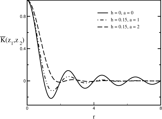
Figure 1: ${\bar{K}}(z_{1},z_{2})$ (85) at $x=y_{1}=y_{2}=0$.

The spectral density at the center of the band is given by,

$$\rho(y)=K(z=iy/{\sqrt{n}},z=iy/{\sqrt{n}})=\frac{2n}{\pi a}\frac{1}{\sqrt{2\pi}}\left[e^{-\frac{2y^{2}}{a^{2}}}\int_{0}^{1}dte^{-\frac{a^{2}t^{2}}{2}}\cosh(2ty)+\frac{\pi h}{a\sqrt{2\pi}}\right.$$ (83)

$$\left.\int_{0}^{\infty}dt\left(\frac{\sin t}{\sinh(\pi ht/2)}-\frac{\sin t}{\pi ht/2}\right)e^{-\frac{t^{2}}{2a^{2}}}\cos(2yt/a^{2})\right]$$

where $y_{1}=y_{2}=y$. The integral over ${\rm Im}(z)$ of the spectral density is given by

$$\int_{-\infty}^{\infty}K(z,z)d{\rm Im}z = \frac{1}{\sqrt{n}}\int_{-\infty}^{\infty}\rho(y)dy$$ (84)

$$= \frac{\sqrt{n}}{\pi}$$

In Fig. 1, we show the normalized kernel ${\bar{K}}(z_{1},z_{2})$ defined by

$${\bar{K}}(z_{1},{z_{2}})=\frac{K(z_{1},{z_{2}})}{\sqrt{\rho(z_{1})\rho(z_{2})}}$$ (85)

for $h=0.15$ and different values of the nonhermiticity parameter. We find that the spectral correlations weaken for increasing values of $a$ and approach the result for the Ginibre ensemble for $a\approx 2$. Although not shown in the picture, it was verified numerically that the exact result (LABEL:copon) is almost indistinguishable from the small $h$ result (82) for values of $h$ up to $h\sim 0.3$, and significant differences are only found for values of $h$ as large as $h\approx 1$. The normalized critical kernel for Hermitian ensembles [37] is easily reproduced from the ratio (85) starting from the expression (81) and taking the limit $a\to 0$,

$$\bar{K}(z_{1},z_{2})\to\frac{\pi h}{2}\frac{\sin(\pi r)}{\sinh(\pi^{2}rh/2)}.$$ (86)

If we consider the $a\to 0$ limit of the kernel (82) or the spectral density (83), $\delta$-functions of the imaginary part of the eigenvalues have to be taken into account carefully. For example, the $a\to 0$ limit of the spectral density (83) is given by

$$\rho(z)=\frac{n}{\pi}\delta(y).$$ (87)

Finally, let us mention that for $a\gg 1$ we recover the Ginibre’s kernel for general complex matrices.

4.2 Correlations at the edge

Next we consider a microscopic scaling limit at the vicinity of either edge of the band of eigenvalues for $z\sim\pm 2\sqrt{n}$, as an extension of edge correlation of the Hermitian Random Matrix ensembles.

We shall need a more refined asymptotic formula for the incomplete $\Gamma$-function than Eq. (73). For $x{>\atop\sim}m$ and $m\gg 1$, the incomplete $\Gamma$-function is dominated by the contribution from the lower end point, so that [51, 27]

$$\Gamma(m+1,x)={\rm e}^{-x}\frac{x^{m+1}}{x-m}\left[1+O\left(\frac{m}{(x-m)^{2}}\right)\right].$$ (88)

Accordingly, the kernel at zero temperature (4.1) reads

$$K_{m}^{0}(z_{1},z_{2}) \simeq \frac{1}{2\pi^{2}\tau\sqrt{1-\tau^{2}}}{\rm e}^{-\frac{1}{2(1-\tau^{2})}[|z_{1}|^{2}+|z_{2}^{2}|-\frac{\tau}{2}(z_{1}^{2}+z_{2}^{2}+z_{1}^{*2}+z_{2}^{*2})]+\frac{1}{2\tau}(z_{1}^{2}+z_{2}^{*2})}$$ (89)

$$\times\int_{-\infty}^{\infty}\int_{-\infty}^{\infty}\frac{dr\,ds}{rs-m}{\rm e}^{(-r^{2}/2+irz_{1}-s^{2}/2-isz^{*}_{2})/\tau+(m+1)\log rs-\log m!}.$$

For $z_{1},z_{2}\sim 2\sqrt{n}$, $m\sim n$, and $\tau\sim 1$, the two saddle points of the $r$ ($s$) integral merge at $r=i\sqrt{n}$ ($s=-i\sqrt{n}$). In order to obtain a nontrivial result, we magnify this region according to the scaling

$$z_{i} = 2\sqrt{n}+\frac{x_{i}}{n^{1/6}}+i\frac{y_{i}}{n^{1/2}},$$

$$m = n+{n^{1/3}}t,$$ (90)

$$\tau^{2} = 1-\frac{\alpha^{2}}{n},$$

and change the integration variables as

$$r=i\sqrt{n}+n^{1/6}p,\quad s=-i\sqrt{n}-n^{1/6}q.$$ (91)

The subleading terms in (88) are of order $O(n^{-1/6})$ in this scaling limit and can be ignored. To the leading order in $n$ we obtain

$$K_{m}^{0}(z_{1},z_{2}) = \sqrt{\frac{2}{\pi}}\frac{n^{1/3}}{a}{\rm e}^{i(y_{1}-y_{2})-\frac{1}{a^{2}}(y_{1}^{2}+y_{2}^{2})}\int_{-\infty}^{\infty}\int_{-\infty}^{\infty}\frac{dp}{2\pi}\frac{dq}{2\pi}\frac{{\rm e}^{i\frac{p^{3}}{3}+ip{(x_{1}-t)}+i\frac{q^{3}}{3}+iq{(x_{2}-t)}}}{-i(p+q)}$$ (92)

$$= \sqrt{\frac{2}{\pi}}\frac{n^{1/3}}{a}{\rm e}^{i(y_{1}-y_{2})-\frac{1}{a^{2}}(y_{1}^{2}+y_{2}^{2})}\int_{-\infty}^{t}\!dt^{\prime}\,{\rm Ai}(x_{1}-t^{\prime}){\rm Ai}(x_{2}-t^{\prime}).$$

where ${\rm Ai}(x)$ is the Airy function

$${\rm Ai}(x)=\int_{{-\infty}}^{{\infty}}\frac{dp}{2\pi}{\rm e}^{i\frac{p^{3}}{3}+ipx}=\int_{0}^{{\infty}}\frac{dp}{\pi}\cos\Bigl{(}\frac{p^{3}}{3}+px\Bigr{)}.$$ (93)

The integral in Eq. (92) is called the Airy kernel $K_{\rm Ai}(x_{1}-t,x_{2}-t)$ (See Ref.[2], §18), describing the edge correlations of the Gaussian Unitary Ensemble. By partial integrations one may express it in an alternative and more familiar form

$$K_{{\rm Ai}}({x_{1}},{x_{2}})=\frac{{\rm Ai}(x_{1}){\rm Ai}^{\prime}(x_{2})-{\rm Ai}^{\prime}(x_{1}){\rm Ai}(x_{2})}{x_{1}-x_{2}}.$$ (94)

The scaling of $m$ in (90) requires the introduction of a finite temperature parameter $h$ by

$$\beta=\frac{1}{n^{1/3}h},$$ (95)

in contrast to the bulk scaling (78). After replacing the sum over $m$ by an integral over $t$, the low-temperature limit of the kernel (69) is given by

$$K(z_{1},z_{2}) = \sqrt{\frac{2}{\pi}}\frac{n^{1/3}}{a}{\rm e}^{i(y_{1}-y_{2})-\frac{1}{a^{2}}(y_{1}^{2}+y_{2}^{2})}\int_{-n^{2/3}}^{\infty}dt\,K_{{\rm Ai}}(x_{1}-t,x_{2}-t)\frac{d}{dt}\left(\frac{1}{1+e^{t/h}}\right)$$ (96)

$$= \sqrt{\frac{2}{\pi}}\frac{n^{1/3}}{a}{\rm e}^{i(y_{1}-y_{2})-\frac{1}{a^{2}}(y_{1}^{2}+y_{2}^{2})}\int_{-\infty}^{\infty}dt\frac{{\rm Ai}(x_{1}-t){\rm Ai}(x_{2}-t)}{1+e^{t/h}}.$$

Due to the different orders of the level spacings in real and imaginary directions, the zero-temperature kernel is factorized, unlike the bulk kernel Eq. (52) of [30] or our Eq. (76). Namely, the dependence of $K^{0}_{m}$ on the order $m$ is merely to dilate the eigenvalue support, which can be compensated by a change of the real part of the eigenvalue coordinate, $x\to x-t$. Accordingly, the effects of nonhermiticity and finite temperature are factorized. The former is reflected in the scaled kernel as a Gaussian blurring in the $y$-direction whereas, as the temperature $h$ increases, the oscillation of the scaled spectral density along the $x$-direction is weakened toward the Poissonian limit. This is shown in Fig. 2 where we plot the spectral density in the Hermitian limit given by $\rho(x)=\int dt\,{\rm Ai}(x-t)^{2}/(1+{\rm e}^{t/h})$.

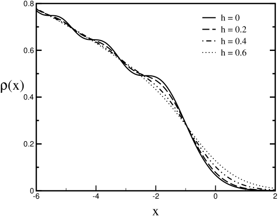
Figure 2: The spectral density at the edge for different values of the temperature parameter, at zero nonhermiticity.

5 Number variance

The number variance in an arbitrary domain $A$ of the complex plane is given by,

$$\Sigma_{2}(L)~{}=~{}L-\int_{A}d^{2}z_{1}\int_{A}d^{2}z_{2}Y_{2}(z_{1},z_{2})\qquad{\rm with}\qquad L=\int_{A}d^{2}z\rho(z),$$ (97)

where $\rho(z)=K(z,z)$, $Y_{2}(z_{1},z_{2})=|K(z_{1},z_{2})|^{2}$ and $K(z_{1},z_{2})$ is the spectral kernel defined in (LABEL:copon). Apart from edge correlations we have found that in the strong nonhermiticity case the two-point correlations decay exponentially on a scale of one level spacing or less which results in an asymptotic linear dependence of the number variance on $A$ with unit slope. Below we focus our analysis on the more interesting weak nonhermiticity limit.

As will be seen in the figures below, the fluctuations of the eigenvalues increase with both increasing temperature $h$ and increasing degree of week nonhermiticity $a$. The reasons for such behavior are the following: For larger values of $h$, the correlations of distant eigenvalues are suppressed resulting in stronger fluctuations and the slope of the asymptotically linear number variance increases with $h$. By increasing the degree of nonhermiticity, eigenvalues have more room to avoid each other along the imaginary axis. As a consequence, spectral fluctuations are stronger and deviations from Wigner statistics are observed.

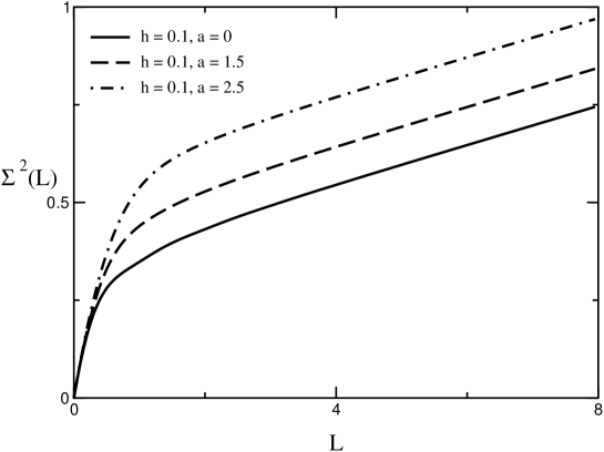
Figure 3: The small $h$ behavior of the number variance $\Sigma^{2}(L)$ versus $L$ given in (5) for $h=0.1$ and values of the nonhermiticity parameter as given in the legend of the figure.

In the limit $h\ll 1$ we calculate the number variance for the area $A=[-L_{x}/2,L_{x}/2]\times(-\infty,\infty)$. Because of the normalization integral (84) we choose $L_{x}=L\pi/\sqrt{n}$ so that the area $A$ contains $L$ eigenvalues on average. The dependence of the kernel on $x$ is subleading in the thermodynamic limit. This allows us to rewrite the number variance as

$$\Sigma^{2}(L)=L-\frac{2\pi}{n^{3/2}}\int_{0}^{L}dr(\pi L/\sqrt{n}-\pi r/\sqrt{n})\int_{-\infty}^{\infty}\int_{-\infty}^{\infty}dy_{1}dy_{2}|K(z_{1},z_{2})|^{2},$$ (98)

where the prefactor includes a contribution from the Jacobian of the transformation (4.1). The integrals over $y_{1}$ and $y_{2}$ are easily performed in terms of the variables $u\equiv y_{1}+y_{2}$ and $v\equiv y_{1}-y_{2}$. The final result for the small $h$ limit of the number variance is thus given by

$$\Sigma^{2}(L)=L-2\int_{0}^{L}dr(L-r)\left[\frac{\sin^{2}(\pi r)}{{\pi}^{2}r^{2}}e^{-\frac{a^{2}r^{2}}{L^{2}}}\right.+$$

$$\left.\frac{\pi^{2}h^{2}}{4}\frac{1}{a\sqrt{\pi}}\int_{-\infty}^{\infty}dt\left(\frac{\sin^{2}(t)}{\sinh^{2}(\pi ht/2)}-\frac{\sin^{2}(t)}{(\pi ht/2)^{2}}\right)e^{-\frac{1}{a^{2}}(t-\pi r)^{2}}\right].$$ (99)

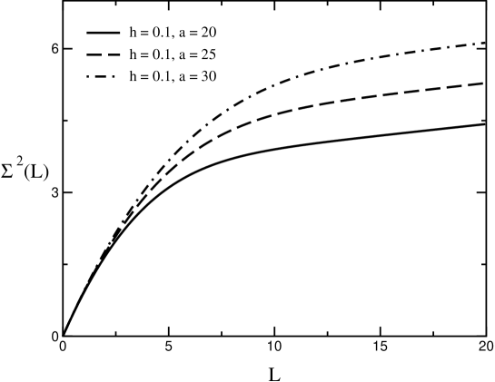
Figure 4: The number variance (5) is computed for large values of the nonhermiticity parameter $a$.

We observe that in this limit the finite temperature effects decouple from the weak nonhermiticity corrections. For $L\gg 1/h$ and $a\ll L$ it can be shown from (5) that the number variance is given by

$$\Sigma^{2}(L)=\frac{a}{\pi^{3/2}}-\frac{\gamma}{\pi^{2}}+\frac{h}{2}L+O(1/L),$$ (100)

where $\gamma$ is the Euler constant. The term linear in $a$ can be calculated in the $h\to 0$ limit and was obtained in [30], whereas the term linear in $h$ can be calculated for $a\to 0$ and was derived in [37]. In Fig. 3, we show the small $h$ limit of the number variance (5) for $h=0.1$ and different values of the nonhermiticity parameter. We observe that the asymptotic linear behavior given by (100) is already reached well below the expected scale of $1/h$. We remark that for values of $h$ as large as $0.3$ the small $h$ result (97) is still very close to the exact result obtained with the kernel (LABEL:copon).

Figure 5: The renormalized spectral density $\rho_{r}(y)=\rho(y)/\rho(0)$ (with $\rho(y)$ defined in (83) in the center of the band is shown for different values of the nonhermiticity parameter.

The small $h$ result for the number variance (5) is also valid for large values of the nonhermiticity parameter. Plots of (5) for $a\gg 1$ are shown in Fig. 4. We find that the asymptotic result for the slope is still approximately given by $h/2$ and depends only weakly on $a$. For $L\ll a$ we find that $\Sigma^{2}(L)\to L$ which is the result for strong nonhermiticity. This crossover behavior was first found in the limit $h\to 0$ [30].

The imaginary part of the eigenvalues is of order $a$. This is shown in Fig. 5 where we plot the $\rho(y)/\rho(0)$ (with $\rho(y)$ given in eq. (83)) versus $y$. Since the imaginary part of the eigenvalues is of the same order as the spacing of the real part of the eigenvalues, the number variance computed for a rectangle $0<{\rm Im}z<\Delta y\ll a$ is expected to be given by $\Sigma^{2}(L)\to L$ where $L$ is the total number of eigenvalues in the rectangle. This is shown in Fig. 5 where we plot the number variance obtained from (97) using the kernel (82).

6 Conclusions

In this article we have introduced a two parameter ensemble of complex random matrices with no hermiticity conditions imposed. This ensemble interpolates between the Gaussian Unitary Ensemble, the Ginibre ensemble and the Poisson ensemble. Using methods from statistical mechanics and properties of orthogonal polynomials, we have analyzed this ensemble in two different limits: weak nonhermiticity and strong nonhermiticity.

We have shown that the joint eigenvalue distribution of our random matrix model coincides with the diagonal element of the density matrix of a two dimensional gas of spinless fermions in the lowest Landau level at finite temperature. The two parameters of our model have been interpreted in terms of a shape parameter of the two dimensional domain of eigenvalues (or particles) and a temperature.

Figure 6: The number variance given by the general formula (97). The domain of integration is a rectangle in the complex plane containing $L$ eigenvalues and width given by $0<{\rm Im}z<\Delta y$. The nonhermiticity parameter is equal to $a=0.4$ and the value of $h$ is equal $h=0.1$ for all curves. The number variance is almost Poisson for $\Delta y\leq a$.

In the strong nonhermiticity limit, in the bulk of the spectrum, the correlations of the eigenvalues are given by Ginibre statistics and decrease exponentially on the scale of the average level spacing. The situation is different near the surface of the spectrum where, at zero temperature, the correlations decrease as an inverse square law in the direction of the surface. At finite temperature this power-law behavior changes into an exponential behavior. At very high temperatures the surface and the bulk are no longer distinguishable. In that case the two-point correlation function of the unfolded eigenvalues still decays exponentially but with an exponent that is proportional to the temperature. In this way the Poisson limit is recovered at high temperatures.

In the weak nonhermiticity limit there is no clear distinction between bulk and surface and the temperature affects the correlation functions of the eigenvalues. In the low temperature limit we have obtained a closed analytical expression for the two-point correlation function which reproduces critical statistics. We have found that, although level repulsion is still present, the number variance is asymptotically linear with a slope depending on the temperature parameter but not on the nonhermiticity parameter. A remarkable feature is that temperature and weak nonhermiticity effects decouple in this region. Thus critical statistics is not modified by a weak nonhermitian perturbation.

Finally, let us explain a physical prediction of the present model. Since for critical statistics the slope of the number variance is related to the multifractal dimension of the wave function and, in our model, the slope does not depend on the nonhermiticity parameter, we predict that the multifractal dimension of a physical system does not depend on the nonhermiticity parameter either. We thus predict the same multifractal dimensions for open and dissipative systems. A simple model for which this prediction may be tested is a three dimensional disordered system at the critical density of impurities and with several leads attached to it. We thus expect that in the weak nonhermiticity domain the leads do not affect the multifractal dimension of the wavefunctions.

Acknowledgments

This work is was partially supported by the Department of Energy grants No. DE-FG02-92ER40716 (SMN) and DE-FG-88ER40388 (AMG and JJMV).

References

• [1] J. Ginibre, J. Math. Phys. 6 (1965) 440.
• [2] M.L. Mehta, β€œRandom Matrices”, 2nd Ed., Academic Press (San Diego, 1991).
• [3] J.J.M. Verbaarschot, H.A. WeidenmΓΌller and M.R. Zirnbauer, Phys. Rep. 129 (1985) 367.
• [4] Y.V. Fyodorov and B.A. Khoruzhenko, Phys. Rev. Lett. 83 (1999) 65.
• [5] W. John, B. Milek, H. Schanz and P. Seba, Phys. Rev. Lett. 67 (1991) 1949.
• [6] J.B. Kogut, M.A. Stephanov, D. Toublan, J.J.M. Verbaarschot and A. Zhitnitsky, Nucl. Phys. B 582 (2000) 477.
• [7] M.A. Stephanov, Phys. Rev. Lett. 76 (1996) 4472.
• [8] M.A. Halasz, J.C. Osborn and J.J.M. Verbaarschot, Phys. Rev. D 56 (1997) 7059.
• [9] D. Toublan and J.J.M. Verbaarschot, Int. J. Mod. Phys. B 15 (2001) 1404.
• [10] H. Markum, R. Pullirsch and T. Wettig, Phys. Rev. Lett. 83 (1999) 484.
• [11] G. Akemann, Phys. Rev. D64 (2001) 114021.
• [12] N. Hatano and D.R. Nelson, Phys. Rev. Lett. 77 (1996) 570; J. Miller and J. Wang, Phys. Rev. Lett. 76 (1996) 1461.
• [13] K.B. Efetov, Phys. Rev. Lett. 79 (1997) 491; Phys. Rev. B. 56 (1997) 9630.
• [14] R. Grobe, F. Haake and H.-J. Sommers, Phys. Rev. Lett. 61 (1988) 1899.
• [15] F. Haake, F. Izrailev and N. Lehmann, Z. Phys. B 88 (1992) 359.
• [16] R. Grobe and F. Haake, Phys. Rev. Lett. 62 (1989) 2893.
• [17] L.E. Reichl, Z.Y. Chen and M. Millonas, Phys. Rev. Lett. 63 (1989) 2013.
• [18] N. Lehmann and H.-J. Sommers, Phys. Rev. Lett. 67 (1991) 941.
• [19] H.-J. Sommers, A. Crisanti, H. Sompolinsky and Y. Stein, Phys. Rev. Lett. 60 (1988) 1895.
• [20] L. Chau and Y. Yu, Comm. Math. Phys. 196 (1998) 203.
• [21] G. Oas, Phys. Rev. E 65 (1997) 205.
• [22] V.L. Girko, Theory of Random Determinants, Kluwer Academic Publishers, Dordrecht, 1990.
• [23] J. Feinberg and A. Zee, Nucl. Phys. B 504 (1997) 579.
• [24] R.A. Janik, W. Norenberg, M.A. Nowak, G. Papp and I. Zahed, Phys. Rev. E 60 (1999) 2699; B. Mehlig and J.T. Chalker, J. Math. Phys. 41 (2000) 3233.
• [25] J.Β Feinberg and A.Β Zee, Nucl.Β Phys.Β B 552 (1999) 599.
• [26] I.K. Kostov, I. Krichever, M. Mineev-Weinstein, P.B. Wiegmann and A. Zabrodin, hep-th/0005259.
• [27] P.J. Forrester and B. Jancovici, Int. J. Mod. Phys. A 11 (1996) 941.
• [28] P.J. Forrester, Phys. Rep. 301 (1998) 235.
• [29] M.B. Hastings, Nucl. Phys. B 572 (2000) 535.
• [30] Y.V. Fyodorov and H.-J. Sommers, JETP Lett. 63 (1996) 1026.
• [31] Y.V. Fyodorov, B.A. Khoruzhenko and H.-J. Sommers, Phys. Lett. A 226 (1997) 46; Phys. Rev. Lett. 79 (1997) 557.
• [32] Y.V. Fyodorov, H.-J. Sommers and B.A. Khoruzhenko, Annal. Inst. H. PoincarΓ© 68 (1998) 449.
• [33] B.I. Shklovskii, B. Shapiro, B.R. Sears, P. Lambrianides and H.B. Shore, Phys. Rev. B. 47 (1993) 11487.
• [34] K.A. Muttalib, Y. Chen, M.E.H. Ismail and V.N. Nicopoulos, Phys. Rev. Lett. 71 (1993) 471.
• [35] C. Blecken, Y. Chen and K.A. Muttalib, J. Phys. A 27 (1994) L563.
• [36] V.E. Kravtsov and K.A. Muttalib, Phys. Rev. Lett. 79 (1997) 1913.
• [37] M. Moshe, H. Neuberger and B. Shapiro, Phys. Rev. Lett. 73 (1994) 1497.
• [38] A.D. Mirlin, Y.V. Fyodorov, F.-M. Dittes, J. Quezada and T.H. Seligman, Phys. Rev. E 54 (1996) 3221.
• [39] F. Evers and A.D. Mirlin, Phys. Rev. Lett. 84 (2000) 3690.
• [40] J.T. Chalker, V.E. Kravtsov and I.V. Lerner, JETP Lett. 64 (1996) 836.
• [41] J.T. Chalker, I.V. Lerner and R.A. Smith, Phys. Rev. Lett. 77 (1996) 554.
• [42] S.M. Nishigaki, Phys. Rev. E 59 (1999) 2853.
• [43] C.-M. Ho and J.T. Chalker, Phys. Rev. B 54 (1996) 8708; J.-S. Caux, N. Taniguchi and A.M. Tsvelik, Nucl. Phys. B 525 (1998) 671.
• [44] R. Klesse and M. Metzler, Phys. Rev. Lett. 79 (1997) 721; A.M. Tsvelik, cond-mat/0112008.
• [45] J.Β C.Β Osborn and J.Β J.Β Verbaarschot, Phys.Β Rev.Β Lett.Β  81 (1998) 268; J.Β C.Β Osborn and J.Β J.Β Verbaarschot, Nucl.Β Phys.Β B 525 (1998) 738.
• [46] A.M. GarcΓ­a-GarcΓ­a and J.J.M. Verbaarschot, Nucl. Phys. B 586 (2000) 668.
• [47] C. Itzykson and J.-B. Zuber, J. Math. Phys. 21 (1980) 411.
• [48] B. Jancovici, J. Stat. Phys. 80 (1995) 445.
• [49] E.R. Smith, J. Phys. A 15 (1982) 3861.
• [50] P. Di Francesco, M. Gaudin, C. Itzykson and F. Lesage, Int. J. Mod. Phys. A 9 (1994) 4257.
• [51] P. Choquard, B. Piller and R. Rentsch, J. Stat. Phys. 46 (1987) 599.