Large-Deviation Functions for Nonlinear Functionals of a
Gaussian Stationary Markov Process

Abstract

We introduce a general method, based on a mapping onto quantum mechanics, for investigating the large-$T$ limit of the distribution $P(r,T)$ of the nonlinear functional $r[V]=(1/T)\int_{0}^{T}dT^{\prime}\,V[X(T^{\prime})]$, where $V(X)$ is an arbitrary function of the stationary Gaussian Markov process $X(T)$. For $T\to\infty$ at fixed $r$ we obtain $P(r,T)\sim\exp[-\theta(r)T]$, where $\theta(r)$ is a large-deviation function. We present explicit results for a number of special cases including $V(X)=XH(X)$ (where $H(X)$ is the Heaviside function), which is related to the cooling and the heating degree days relevant to weather derivatives.

PACS numbers: 05.70.Ln, 05.40.+j, 02.50.-r, 81.10.Aj

I Introduction

The “persistence” of a continuous stochastic process has been the subject of considerable recent interest among both theoreticians and experimentalists in the field of nonequilibrium processes. Persistence is the probability $P(t)$ that a stochastic variable $x(t)$ of zero mean does not change sign up to time $t$. Systems studied include reaction-diffusion processes, phase-ordering kinetics, fluctuating interfaces and simple diffusion from random initial conditions [1]. Experimental measurements have been carried out on breath figures [2], liquid crystals [3], soap froths [4], and diffusion of Xe gas in one dimension [5]. In “coarsening” systems like these, which do not possess a definite length or time scale, the persistence has a power-law decay, $P(t)\sim t^{-\theta}$, at late times, and the persistence exponent $\theta$ is in general non-trivial. In such systems, the normalized two-time correlation function, $C(t_{1},t_{2})=\langle x(t_{1})x(t_{2})\rangle/[\langle x^{2}(t_{1})\rangle\,\langle x^{2}(t_{2})\rangle]^{1/2}$ has the “scaling” form, $C(t_{1},t_{2})=f(t_{1}/t_{2})$, depending only on the ratio of the two times. In such systems, a simplification is achieved by introducing the logarithmic time-scale $T=\ln t$, and the normalized variable $X(T)=x(t)/\langle x^{2}(t)\rangle^{1/2}$, since the correlation function of $X$ depends only on the time difference $T_{2}-T_{1}$, i.e.  the process $X(T)$ is stationary. Thus one is led to consider stationary stochastic processes. These processes are, of course, also of interest in their own right. In the new time variable, the persistence decays exponentially, $P\sim\exp(-\theta T)$.

In this paper we consider the integrated quantity

$$r=\frac{1}{T}\int_{0}^{T}dT^{\prime}\,V[X(T^{\prime})]$$ (1)

where $V(X)$ is an arbitrary function of the stochastic variable $X(T)$. Hence $r$ is a functional of $V$. For the special case $V(X)=H(X)$, where $H(X)$ is the Heaviside step function, $r$ is just the fraction of time for which $X(T^{\prime})>0$ in the time interval $O\leq T^{\prime}\leq T$. In this case, the probability distribution, $P(r,T)$, of $r$ for given $T$ is just the “residence -time” distribution which, together with the related “sign-time” distribution, where $V(X)={\rm sgn}(X)$, has attracted a lot of attention earlier in the mathematics literature[6, 7] and more recently in the statistical physics community[8]. Here we consider a general function $V(X)$. We restrict our attention, however, to the class of processes where $X(T)$ is a stationary Gaussian Markov process, for which some analytic progress can be made. A case of some interest, which we analyze in detail, is $V(X)=XH(X)$. This case is relevant to weather derivatives as we now explain.

It has been estimated that about 1 trillion dollars of the 7 trillion dollar US economy is weather related [9]. For example, weather conditions directly affect agricultural outputs and the demand for energy products and indirectly affect retail businesses [10]. Weather derivatives, first introduced in 1997, are financial instruments which allow hedging (by, for example, energy suppliers) against adverse weather conditions over a period of time. Here “adverse” might mean an unusually warm winter, when low demand for energy would affect the supplier’s profits, as well as an unusually cold one when the supplier is unable to meet the demand. Temperature derivatives, the most common form of weather derivatives, are based on the concepts of “heating degree days” and “cooling degree days”, which are (rough) measures of the cumulative demand for heating and cooling respectively.

Let $X(T)$ be the temperature at time $T$ in a given city. On a given day, $n$, the mean, $X_{n}$, of the highest and lowest temperatures is recorded. The number of cooling degree days ($CDD$), over a period of $N$ days, is given by $CDD=\sum_{n=1}^{N}\max(X_{n}-X_{o},0)$, where $X_{o}$ is a reference, or baseline, temperature, while the number of heating degree days ($HDD$) is $HDD=\sum_{n=1}^{N}\max(X_{o}-X_{n},0)$. In the present paper we will, for simplicity, use an integral over continuous time rather than a sum, so that the cooling degree days are given by $CDD=\int_{0}^{T}dT^{\prime}\,[X(T^{\prime})-X_{o}]\,H[X(T^{\prime})-X_{o}]$, where $H(X)$ is the Heaviside step function. Thus $CDD$ is the integrated temperature excess (over the reference temperature) restricted to those periods where the temperature is above the reference level. It is a crude measure of the amount of cooling (air conditioning) required during the period $T$ and also of the energy required to produce this cooling. Note that the power consumption of an air conditioner actually varies, for small temperature differences, as the square of the temperature difference between the room and ambient temperatures, so a better measure of the energy required would be $\int_{0}^{T}dT^{\prime}\,[X(T^{\prime})-X_{o}]^{2}\,H[X(T^{\prime})-X_{o}]$, instead of $CDD$. In the notation of this paper, $CDD=rT$, with $V(X)=(X-X_{o})H(X-X_{o})$ in Eq.  (1). The number of heating degree days ($HDD$) is similarly given by $HDD=\int_{0}^{T}dT^{\prime}[X_{o}-X(T^{\prime})]\,H[X_{o}-X(T^{\prime})]$, which is a measure the amount of heating required in the period $T$ and of the energy required to produce this heating. Estimating the likelihood of large deviations from the mean in $CDD$ or $HDD$ is clearly of interest to energy companies.

To make further progress, a realistic statistical model of temperature fluctuations is required. At this stage, however, any realistic model is too intractable to allow analytical progress. To illustrate the general approach we will instead employ a simple, though unrealistic, model in which the temperature, $X(T)$, is taken to be a stationary Gaussian Markov process. We will discuss the limitations of this model, and possible improvements, in the Conclusion. As a further simplification, we take the reference temperature $X_{o}$ to be the mean of $X(T)$, though this simplification is not essential and can be relaxed.

The outline of the paper is as follows. In section II we introduce the general approach to the problem of computing the distribution, $P_{T}(r)$, of the quantity $r$ defined by Eq.  (1). Using a path-integral representation, the calculation of $P_{T}(r)$ is mapped onto a problem in quantum mechanics, in which the function $V(X)$ appears in the potential energy. In the limit of large $T$, only the quantum ground state energy is required. The final result takes the form $P_{T}(r)\sim\exp[-\theta(r)T]$, where the function $\theta(r)$ is a large-deviation function. For the case of the sign-time distribution, corresponding to $V(X)={\rm sgn}(X)$, $r$ lies in the range $-1\leq r\leq 1$, and it is clear that $\theta(1)$ is just the usual persistence exponent, $\theta$, since $r=1$ requires $X(T^{\prime})>0$ for $0\leq T^{\prime}\leq T$. In section III, the method is illustrated on a number of special cases, of which $V(X)=\alpha X$ and $V(X)=\beta X^{2}/2$ are studied first as exactly-soluble tutorial illustrations before turning to the CDD problem (in the simple form outlined above) and finally the sign-time distribution. The last two examples can be solved analytically in various regimes, and numerically elsewhere. Section IV concludes with a discussion and summary of the results.

II GENERAL APPROACH

Consider the general stationary Gaussian Markov process (Ornstein-Uhlenbeck process) $dx/dt=-\mu x+\xi(t)$, where $\xi(t)$ is Gaussian white noise with zero mean, and correlator $\langle\xi(t)\xi(t^{\prime})\rangle=2D\,\delta(t-t^{\prime})$. After the change of variables $t=T/\mu$, $x=(2D/\mu)^{1/2}X$, the equation takes the form

$$\frac{dX}{dT}=-X+\eta(T)\ ,$$ (2)

where $\langle\eta(T)\rangle=0$ and

$$\langle\eta(T)\eta(T^{\prime})\rangle=\delta(T-T^{\prime})\ .$$ (3)

The probability distribution of $X(T^{\prime})$ for $0\leq T^{\prime}\leq T$ is given by

$$P[X]=N\exp\left\{-\frac{1}{2}\int_{0}^{T}dT^{\prime}\left[\dot{X}^{2}(T^{\prime})+X^{2}(T^{\prime})\right]\right\}\ ,$$ (4)

where $\dot{X}(T^{\prime})\equiv dX/dT^{\prime}$, and $N$ is a normalization constant. Our goal is to calculate the probability distribution of $r$, defined by equation (1). In practice it is convenient to look at the distribution $P_{u}(u)$ of the quantity $u=rT$. Its Laplace transform is

$$\tilde{P}_{u}(s)=\langle\exp(-rsT)\rangle=Z(s)/Z(0)\ ,$$ (5)

where $Z(s)$ is given by the path integral

$$Z(s) = \int DX(T)\exp\{-\frac{1}{2}\int_{0}^{T}dT^{\prime}(\dot{X}^{2}+X^{2}$$ (7)

$$\hskip 128.0374pt+2s\,V[X])\}\ .$$

We are interested in the limit $T\to\infty$. It is convenient to impose periodic boundary conditions, $X(T)=X(0)$, since this restriction will not change the results in the large-$T$ limit. Furthermore, the exponential in (4) should strictly contain the combination $(\dot{X}+X)^{2}$ instead of $(\dot{X}^{2}+X^{2})$. The missing term, $2X\dot{X}$, is however a perfect derivative, whose integral vanishes for periodic boundary conditions. Finally, with these boundary conditions the function $Z(s)$ is the imaginary-time Feynman path-integral that gives the partition function of a quantum particle with Hamiltonian ${\cal H}=p^{2}/2+X^{2}/2+sV(X)$ at inverse temperature $T$, $p$ being the canonical momentum conjugate to $X$. For $T\to\infty$ the ground state dominates to give, in this limit,

$$\langle\exp(-rsT)\rangle=\exp\{-T[E(s)-E(0)]\}\ ,$$ (8)

where $E(s)$ is the ground-state energy for the Schrödinger equation

$$-\frac{1}{2}\frac{d^{2}\psi}{dX^{2}}+U(X)\psi=E(s)\psi\ ,$$ (9)

with potential

$$U(X)=X^{2}/2+sV(X)\ .$$ (10)

For $s=0$ the problem reduces to a simple harmonic oscillator, and $E(0)=1/2$.

The stochastic process $x(t)$ studied above corresponds to the position of a Brownian particle in an external potential $\mu x^{2}/2$. For the case of a pure Brownian motion ($\mu=0$), Kac derived a formalism[6] to study the distributions of arbitrary functionals $V[x]$ which also used a mapping to the Schrödinger equation. Note, however, that the method presented above for the $\mu\neq 0$ case differs in details from the original Kac formalism.

To illustrate the method we discuss two simple examples, before turning to some nontrivial cases, including the CDD problem.

III SPECIAL CASES

A $V(X)=\alpha X$

For this case we have

$$u=rT=\alpha\int_{0}^{T}dT^{\prime}\,X(T^{\prime})\ .$$ (11)

This case is actually trivial since $u$, being a sum of zero-mean Gaussian variables, is itself a zero-mean Gaussian variable. All we require, therefore, is the variance, given by

$$\langle u^{2}\rangle=\alpha^{2}\int_{0}^{T}dT_{1}\int_{0}^{T}dT_{2}\,\langle X(T_{1})\,X(T_{2})\rangle\ .$$ (12)

For the Ornstein-Uhlenbeck process (2), with noise correlator (3), one easily finds $\langle X(T_{1})\,X(T_{2})\rangle=(1/2)\exp(-|T_{1}-T_{2}|)$. Inserting this result in (12), and extracting the leading large-$T$ behavior, gives $\langle u^{2}\rangle\to\alpha^{2}T$, and therefore $\langle r^{2}\rangle\to\alpha^{2}/T$. Hence the asymptotic distribution of $r$ is given by (neglecting prefactors)

$$P_{T}(r)\sim\exp(-Tr^{2}/2\alpha^{2})\ ,\ \ \ \ \ T\to\infty\ .$$ (13)

We now show how the general machinery we have set up in section II recovers this result. The potential $U(X)$ in the Schrödinger equation (9) takes the form

$$U(x)=X^{2}/2+s\alpha X=(X+s\alpha)^{2}/2-s^{2}\alpha^{2}/2\ .$$ (14)

This is just a harmonic oscillator with a shifted origin, so $E(s)=1/2-s^{2}\alpha^{2}/2$ and, using (8),

$$\langle\exp(-rsT)\rangle=\exp(Ts^{2}\alpha^{2}/2)$$ (15)

for large $T$. To recover $P_{T}(r)$ we can invert the Laplace transform as follows. Neglecting pre-exponential factors,

$$P_{T}(r)=T\int_{-i\infty}^{i\infty}\frac{ds}{2\pi i}\,\exp[T(rs+s^{2}\alpha^{2}/2)]\ .$$ (16)

This integral can, of course, be evaluated exactly. Here, however, we use the method of steepest descents, which is valid for large $T$ and can be readily generalized to the other, less trivial, cases that we will discuss. Writing the integrand in the form $\exp[Tg(s)]$, we have $g(s)=rs+s^{2}\alpha^{2}/2$. The integral is dominated by the saddle point at $s=-r/\alpha^{2}$, where $g=-r^{2}/2\alpha^{2}$. The integration contour is deformed to pass over the saddle point, which lies on the real $s$ axis. The saddle point is thus a minimum of $g(s)$ with respect to variations of $s$ along the real axis. The final result, ignoring non-exponential prefactors, is identical to (13).

The structure of (13) is

$$P_{T}(r)\sim\exp[-\theta(r)T]\ ,$$ (17)

with

$$\theta(r)=r^{2}/2\alpha^{2}\ .$$ (18)

We can easily generalize this method to arbitrary $V(X)$. The path-integral approach gives the general result (neglecting prefactors)

$$P_{T}(r)\sim\int_{-i\infty}^{i\infty}ds\,\exp[Tg(s)]\ ,$$ (19)

where

$$g(s)=rs+E(0)-E(s)\ .$$ (20)

Using the steepest-descent method for the integral gives

$$\theta(r)=\max_{s}\,\left[E(s)-\frac{1}{2}-rs\right]\ ,$$ (21)

where we have inserted $E(0)=1/2$. The next example is a simple application of this idea.

B $V(X)=\beta X^{2}/2$

This case illustrates the power of the method. The potential energy is now

$$U(X)=(1+\beta s)X^{2}/2\ ,$$ (22)

so we have a harmonic oscillator again but with a modified frequency, $\omega=(1+\beta s)^{1/2}$, giving $E(s)=(1+\beta s)^{1/2}/2$. Thus

$$\theta(r) = \max_{s}\,\left[\frac{1}{2}(1+\beta s)^{1/2}-\frac{1}{2}-rs\right]$$ (23)

$$= \left(\sqrt{\frac{r}{\beta}}-\frac{1}{4}\sqrt{\frac{\beta}{r}}\right)^{2}\ .$$ (24)

Note that $\theta(r)$ now has its minimum at $r=\beta/4$, which is just the mean value of $r$ [noting that $\langle X^{2}\rangle=1/2$ follows from (2) and (3)], while large ($r\to\infty$) and small ($r\to 0$) values of $r$ are strongly suppressed. An expansion of $\theta$ near its minimum value gives a Gaussian distribution $P_{T}(r)\sim\exp[-4T(r-\beta/4)^{2}/\beta^{2}]$. This agrees with the result expected from the central limit theorem, i.e.  $P_{T}(r)\sim\exp[-(r-\mu)^{2}/2\sigma^{2}]$, with mean $\mu=\beta/4$ and variance $\sigma^{2}=\beta^{2}/8T$. For $T\to\infty$, the distribution becomes very narrow such that, at fixed $r$, the central limit theorem fails to give the correct asymptotics. The form (17) thus gives the behavior in the extreme tails of the distribution at large $T$. The function $\theta(r)$ is a “large-deviation function” which controls the distribution of $r$ for large $T$.

We note that this special case with $V(X)=\beta X^{2}/2$ was also studied recently by Farago[11] in the context of power fluctuations in the Langevin equation (2) by a somewhat different method. The probability density function of the dissipated power in reference[11] is precisely the distribution $P_{T}(r)$ studied here and the corresponding large-deviation function $\theta(r)$ has the same expression as in Eq. (24). However our derivation seems simpler and easily generalizable to other forms of $V(X)$ as we show below.

C $V(X)=XH(X)$: “Cooling Degree Days”

In this case the quantity $rT$ gives the integrated value of $X$ over the interval $T$, restricted to those values where $X>0$. If $X$ is the excess temperature over some baseline value where cooling becomes necessary, $rT$ is a crude measure of the total energy consumption required to provide the cooling [$V(X)=X^{2}H(X)$ would be a better measure, as discussed in the Introduction]. In the present simple model we have taken the mean temperature equal to the reference temperature (with $X(T)$ being the deviation from the mean), though this is not an essential restriction. The Schrödinger equation (9) takes the form

$$\psi^{\prime\prime}-X^{2}\psi-2sX\psi+2E(s)\psi = 0,\ \ \ X\geq 0\ ,$$ (25)

$$\psi^{\prime\prime}-X^{2}\psi+2E(s)\psi = 0,\ \ \ X\leq 0\ ,$$ (26)

where $\psi^{\prime\prime}\equiv d^{2}\psi/dX^{2}$. The required solutions can be expressed in terms of parabolic cylinder functions, ${\rm D}_{p}(x)$, using the standard solutions of the parabolic cylinder equation $y^{\prime\prime}-(x^{2}/4+a)y=0$ [12]. Selecting the solutions that satisfy the physical boundary condition $\psi(\pm\infty)=0$ gives

$$\psi(X) = \psi_{+}(X)=A\,{\rm D}_{p_{+}}\left(\sqrt{2}(X+s)\right),\ \ \ X\geq 0\ ,$$ (27)

$$= \psi_{-}(X)=B\,{\rm D}_{p_{-}}\left(-\sqrt{2}X\right),\ \ \ X\leq 0\ ,$$ (28)

where $A$, $B$ are constants and

$$p_{+} = E(s)-\frac{1}{2}+\frac{s^{2}}{2}\ ,$$ (29)

$$p_{-} = E(s)-\frac{1}{2}\ .$$ (30)

The ratio $A/B$ and the energy eigenvalues $E(s)$ are obtained from matching the wavefunction and its derivative at $X=0$, i.e.  we require $\psi_{+}(0)=\psi_{-}(0)$ and ${\psi_{+}}^{\prime}(0)={\psi_{-}}^{\prime}(0)$. This yields the eigenvalue equation

$$\frac{{{\rm D}_{p_{+}}}^{\prime}(\sqrt{2}s)}{{\rm D}_{p_{+}}(\sqrt{2}s)}=-\frac{{{\rm D}_{p_{-}}}^{\prime}(0)}{{\rm D}_{p_{-}}(0)}\ .$$ (31)

The determination of $E(s)$ from these equations is not possible analytically for general $s$. However, in the regimes $s\to\infty$, and $s\to-\infty$, which determine the small-$r$ and large-$r$ behavior respectively of $\theta(r)$, analytical progress is possible. We consider these in turn.

1 The limit $r\to\infty$

As we shall see, in this limit it is sufficient to compute $E(s)$ in the limit $s\to-\infty$. This can either be done directly from (31), or using the following (simpler) physical argument.

Recall that, for $V(X)=XH(X)$, the potential $U(X)$ in the Schrödinger equation is

$$U(X) = X^{2}/2+sX\ ,\ \ \ X\geq 0\ ,$$ (32)

$$= X^{2}/2\ ,\ \ \ X\leq 0\ .$$ (33)

For $s\to-\infty$, the potential has a deep minimum, of depth $-s^{2}/2$, located at $X=-s$. The wavefunction is exponentially small at $X=0$, $\psi(0)\sim\exp(-s^{2}/2)$, and the change in the potential in the regime $X<0$ has an exponentially small effect on the ground state energy. Thus

$$E(s)=-s^{2}/2+1/2+O(e^{-s^{2}}),\ \ \ s\to-\infty\ .$$ (34)

The same result can be obtained, after some algebra, directly from (31). Inserting the result in (21) gives $\theta(r)=\max_{s}(-s^{2}/2-rs)=r^{2}/2$. Since the maximum occurs at $s=-r$, the calculation is self-consistent for $r\to\infty$. Thus we obtain

$$\theta(r)\to r^{2}/2\ ,\ \ \ \ r\to\infty\ .$$ (35)

This large-$r$ result has the same form as equation (18), which gives the general-$r$ result for potential $V(X)=\alpha X$ (with $\alpha=1$ here). This correspondence is not so surprising: For $r\to\infty$, the dominant processes $X(T^{\prime})$, for $0\leq T^{\prime}\leq T$, will correspond to large positive $X$, so the step function $H(X)$ in $V(X)$ plays no role in this limit.

2 The limit $r\to 0$

We shall see that this limit corresponds to $s\to\infty$. Again, one can use physical arguments as a short cut. For $s\to\infty$, one has $U(X)=X^{2}/2$ for $X<0$, with essentially a hard wall at $X=0$. This gives, to leading order, $E(s)\to 3/2$. We need, however, the leading correction to this result. Since the wave function does not penetrate far into the wall, we can neglect the $X^{2}$ term in the potential for $X>0$, i.e.  write $U(X)=sX$. The Schrödinger equation then simplifies to

$$\psi^{\prime\prime}-2sX\,\psi+2E(s)\psi = 0\ ,\ \ \ X\geq 0\ ,$$ (36)

$$\psi^{\prime\prime}-X^{2}\psi+2E(s)\psi = 0\ ,\ \ \ X\leq 0\ .$$ (37)

The wavefunction for $X\leq 0$ is again a parabolic cylinder function, while for $X\geq 0$ it can be expressed as an Airy function:

$$\psi(X) = A\,{\rm Ai}\left((2s)^{1/3}X\right)\ ,\ \ \ X\geq 0\ ,$$ (38)

$$= B\,{\rm D}_{p_{-}}\!\left(-\sqrt{2}X\right)\ ,\ \ \ X\leq 0\ ,$$ (39)

where $A$, $B$ are constants, and $p_{-}=E(s)-1/2$ as before. Matching the wavefunction and its first derivative at $X=0$ gives the eigenvalue equation

$$\frac{(2s)^{1/3}{\rm Ai}^{\prime}(0)}{\sqrt{2}{\rm Ai}(0)}=-\frac{{{\rm D}_{p_{-}}}^{\prime}(0)}{{\rm D}_{p_{-}}(0)}=\frac{\sqrt{2}{\rm\Gamma}\left(\frac{1-p_{-}}{2}\right)}{{\rm\Gamma}\left(-\frac{p_{-}}{2}\right)}\ ,$$ (40)

where ${\rm\Gamma}(x)$ is the Gamma function. In the limit $s\to\infty$, the left-hand side of (40) tends to infinity, so the right-hand side (RHS) must also diverge in this limit. The ground state corresponds to the first divergence, where $p_{-}\to 1$. Therefore we write $p_{-}=1-\epsilon$ in (40), and seek the leading behavior as $\epsilon\to 0$. This gives ${\rm RHS}\to-(2/\pi)^{1/2}/\epsilon$. Inserting this result in (40) gives, to leading order,

$$\epsilon = -2^{1/6}\sqrt{\frac{2}{\pi}}\,\frac{{\rm Ai}(0)}{{\rm Ai}^{\prime}(0)}\,s^{-1/3}$$ (41)

$$= \sqrt{\frac{2}{\pi}}\,\frac{2^{1/6}}{3^{1/3}}\,\frac{{\rm\Gamma}(1/3)}{{\rm\Gamma}(2/3)}\,s^{-1/3}\equiv a\,s^{-1/3}\ ,$$ (42)

the last equation defining the constant $a$. Finally we have $E(s)=p_{-}+1/2=3/2-\epsilon$. Inserting this in (21) gives, for $r\to 0$,

$$\theta(r)=\max_{s}(1-as^{-1/3}-rs)=1-br^{1/4}\ ,$$ (43)

where

$$b=4\left(\frac{a}{3}\right)^{3/4}=\frac{4\sqrt{2}}{3\pi^{3/8}}\,\left(\frac{{\rm\Gamma}(1/3)}{{\rm\Gamma}(2/3)}\right)^{3/4}=2.04763\ldots$$ (44)

Note that the value of $s$ at which the maximum occurs in (43) is $s=(a/3r)^{3/4}$, justifying our use of a large-$s$ analysis of $E(s)$ for the limit $r\to 0$.

That $\theta(r)\to 1$ for $r\to 0$ is intuitively clear, since $r=0$ requires $X(T)\leq 0$ for all $T$. This reduces to the usual persistence probability of the Markov process (2), for which $\theta=1$.

3 $\theta(r)$ for $r$ near $\langle r\rangle$

Equations (35) and (43) give analytical results for $\theta(r)$ in the limits of large and small $r$ respectively. For general $r$, $\theta$ has to be computed numerically. There is, however, one other regime where analytical progress is possible, namely for $r$ close to its mean value, where the central limit theorem (CLT) applies.

The mean value is given by

$$\langle r\rangle = \langle V(X)\rangle=\langle XH(X)\rangle\$$ (45)

$$= \frac{1}{2}(\langle X\rangle+\langle|X|\rangle)\ .$$ (46)

The Gaussian distribution for $X$ gives immediately $\langle X\rangle=0$ and $\langle|X|\rangle=\sqrt{2/\pi}\langle X^{2}\rangle^{1/2}=1/\sqrt{\pi}$. Thus

$$\langle r\rangle=\frac{1}{2\sqrt{\pi}}\ .$$ (47)

In a similar way, the variance of $r$ can be calculated, by exploiting the Gaussian properties of the process $X(T)$. A tedious but straightforward calculation gives, for $T\to\infty$,

$$\sigma^{2}\equiv\langle r^{2}\rangle-\langle r\rangle^{2}=\frac{1}{2\pi T}\,\left(\pi+\ln 2-2\right)\ .$$ (48)

The central limit theorem then gives the behavior of $P_{T}(r)$ for $r$ near $r_{c}$ as $P_{T}(r)=(2\pi\sigma^{2})^{-1/2}\exp[-(r-\langle r\rangle)^{2}/2\sigma^{2}]$. Inserting the explicit expressions for $\langle r\rangle$ and $\sigma^{2}$ gives $P_{T}(r)\sim\exp[-\theta(r)T]$, with

$$\theta(r)=\left(\frac{\pi}{\pi+\ln 2-2}\right)\,\left(r-\frac{1}{2\sqrt{\pi}}\right)^{2}\ ,$$ (49)

correct to leading nontrivial order in $(r-\langle r\rangle)$.

The full result for $\theta(r)$ can be obtained by numerically solving (31) for the ground state energy $E(s)$ for each value of $r$, then using (21) to find the corresponding $\theta(r)$. The result is displayed in Figure 1, with the asymptotic forms for $r\to\infty$ and $r\to 0$ indicated. Note the very sharp rise to the value unity as $r\to 0$, as indicated by Eq. (43).

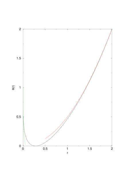
FIG. 1.: The function $\theta(r)$ for the CDD problem, showing the asymptotic behavior for small and large $r$.

In terms of the CDD problem, the behavior below the minimum (i.e. for $r<\langle r\rangle$) determines the probability of an unusually small $CDD$ (“cool summer”), while the region above the minimum corresponds to an unusually large $CDD$ (“hot summer”). The fact that the function $\theta(r)$ initially increases less rapidly to the right of the minimum than to the left indicates that (within this very simple model) summers with a slightly larger than average $CDD$ are more probable than those with a slightly smaller than average $CDD$. This asymmetry is a consequence of the nonlinear relation between $CDD$ and the temperature fluctuations, which are symmetric about the mean in our model. It should be stressed that the integration period $T$ has been taken to be large, to justify the steepest descent calculation. In practice this means that $T$ (the length of a summer, say) must be large compared to the correlation time of the temperature (a few days, perhaps), which is not totally unreasonable.

D $V(X)={\rm sgn}(X)$: The “Sign-Time Distribution”

The structure of the calculation is similar to that of the preceding subsection. The Schrödinger equation is

$$\psi^{\prime\prime}-X^{2}\psi-2[s-E(s)]\psi = 0,\ \ \ X>0\ ,$$ (50)

$$\psi^{\prime\prime}-X^{2}\psi+2[s+E(s)]\psi = 0,\ \ \ X<0\ .$$ (51)

The solutions are parabolic cylinder functions,

$$\psi(X) = \psi_{+}(X)=A\,{\rm D}_{p+}(\sqrt{2}X)\ ,\ \ \ X\geq 0\ ,$$ (52)

$$= \psi_{-}(X)=B\,{\rm D}_{p_{-}}(-\sqrt{2}X)\ ,\ \ \ X\leq 0\ .$$ (53)

where now

$$p_{\pm}=E(s)\mp s-1/2\ .$$ (54)

Matching the wavefunction and its derivative at $X=0$ gives the eigenvalue equation

$$\frac{{{\rm D}_{p_{+}}}^{\prime}(0)}{{\rm D}_{p_{+}}(0)}=-\frac{{{\rm D}_{p_{-}}}^{\prime}(0)}{{\rm D}_{p_{-}}(0)}\ ,$$ (55)

which, using standard identities relating ${\rm D}_{p}(0)$ and ${{\rm D}_{p}}^{\prime}(0)$ to gamma functions [12], reduces to

$$\frac{{\rm\Gamma}\left(\frac{1-p_{+}}{2}\right)}{{\rm\Gamma}\left(-\frac{p_{+}}{2}\right)}=-\frac{{\rm\Gamma}\left(\frac{1-p_{-}}{2}\right)}{{\rm\Gamma}\left(-\frac{p_{-}}{2}\right)}\ .$$ (56)

Although this equation cannot be solved analytically for general $s$, the limits $s\to 0$ and $s\to\infty$ are tractable. Note that $E(s)=E(-s)$ by symmetry, so there is no need to consider $s\to-\infty$ separately.

The analysis starts from the potential well, $U(X)=X^{2}/2+s\,{\rm sgn}(X)$. For small $s$, the ground state energy $E(s)$ is perturbatively close to, but slightly smaller than, $E(0)=1/2$. Therefore we write

$$E(s)=1/2-\delta(s)\ ,$$ (57)

where we anticipate $\delta(s)=O(s^{2})$ from the symmetry $E(s)=E(-s)$. Inserting this form in (54), (56) becomes

$$\frac{{\rm\Gamma}\left(\frac{1+s+\delta}{2}\right)}{{\rm\Gamma}\left(\frac{s+\delta}{2}\right)}=-\frac{{\rm\Gamma}\left(\frac{1-s+\delta}{2}\right)}{{\rm\Gamma}\left(\frac{-s+\delta}{2}\right)}\ .$$ (58)

Expanding to fourth order in $s$ and second order in $\delta$ gives

$$\delta=s^{2}\,\ln 2-cs^{4}+O(s^{6})\ ,$$ (59)

where

$$c=\frac{1}{3}(\ln 2)^{3}+\frac{\pi^{2}}{12}\ln 2-\frac{1}{4}{\rm\zeta}(3)=0.269865\ldots\ ,$$ (60)

and ${\rm\zeta}(n)$ is the Riemann zeta function. Inserting this result in (21) gives

$$\theta(r) = \max_{s}[-rs-s^{2}\ln 2+cs^{4}+O(s^{6})]$$ (61)

$$= \frac{r^{2}}{4\ln 2}+c\left(\frac{r}{2\ln 2}\right)^{4}+O(r^{6})\ .$$ (62)

The maximum occurs at $s=-r/2\ln 2+O(r^{3})$, so our study at small $s$ is self-consistent at small $r$.

For $s\to\infty$, on the other hand, the potential develops a hard wall at the origin, and has a depth of $-s$ next to the wall. Therefore we write $E(s)=-s+3/2-\epsilon$, with $\epsilon$ small. Putting this form in (54), (56) becomes

$$\frac{{\rm\Gamma}[s+\epsilon/2]}{{\rm\Gamma}[s+(\epsilon-1)/2]}=-\frac{{\rm\Gamma}[\epsilon/2]}{{\rm\Gamma}[(\epsilon-1)/2]}\ .$$ (63)

Taking the limits $s\gg 1$, and $\epsilon\ll 1$ readily leads to

$$\epsilon=(\pi s)^{-1/2}$$ (64)

to leading order for large $s$. Using this in (21) gives

$$\theta(r) = \max_{s}[1-(1+r)s-1/(\pi s)^{1/2}]$$ (65)

$$= 1-\frac{3}{2}\left(\frac{2}{\pi}(1+r)\right)^{1/3}+\cdots$$ (66)

The maximum occurs at $s=[2\sqrt{\pi}(1+r)]^{-2/3}]$, which tends to infinity as $r\to-1$ so the calculation is self-consistent in this limit. The symmetry of the problem under $r\to-r$ leads to the more general result

$$\theta(r)=1-\frac{3}{2}\left(\frac{2}{\pi}(1-|r|)\right)^{1/3}+\cdots\ ,\ \ \ \ r\to\pm 1\ .$$ (67)

The function $\theta(r)$ is plotted in Figure 2, with only the region $r\geq 0$ shown explicitly. The limiting behavior for small $r$ and $r$ close to unity is also shown.

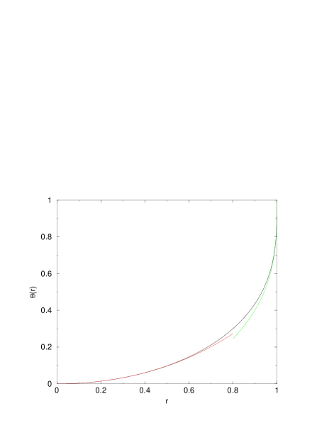
FIG. 2.: The function $\theta(r)$ for the sign-time distribution, showing the limiting behavior for $r\to 0$ and $r\to 1$.

IV Conclusion

In this paper we have presented a general method for computing the asymptotic behavior of the the probability distribution of the quantity $r=(1/T)\int_{0}^{T}dT^{\prime}\,V[X(T^{\prime})]$, where $V(X)$ is an arbitrary function and $X(T)$ is an Ornstein-Uhlenbeck stochastic process representing the motion of a Brownian particle in the presence of a stable parabolic potential $\mu X^{2}/2$. The main new result is that for $\mu>0$, the distribution of $r$, for large window size $T$ has the form $P_{T}(r)\sim\exp[-\theta(r)T]$, where $\theta(r)$ is the large-deviation function. The calculation proceeds via a mapping onto a quantum mechanical problem described by the Schrödinger equation (9) for a particle moving in the potential (10), where $s$ is the Laplace variable conjugate to $rT$. The inverse Laplace transform can be performed using steepest descents in the limit $T\to\infty$.

Two non-trivial applications have been presented. The first is a calculation of the large-deviation function $\theta(r)$ for the cooling degree days problem, based on a simple model of temperature fluctuations. The model used assumes that the temperature fluctuation $X(T)$ is described by the Ornstein-Uhlenbeck process (2), i.e.  that $X(T)$ is a stationary Gaussian Markov process with time-independent noise strength. This may not be a realistic model for several reasons: (i) A simple Markov process is not thought to be an optimized model of temperature fluctuations, which tend to exhibit stronger autocorrelations than a Markov process. A more plausible statistical model, according to [10], writes the fluctuation, $X_{n}$, of the mean (average of daily high and low) temperature on day $n$ as the linear combination $X_{n}=\sum_{m=1}^{k}w_{n-m}\,X_{m}+\eta_{n}$, where the “memory kernel” $w_{n-m}$ is a decreasing function of $n-m$ and $\eta_{n}$ is uncorrelated Gaussian noise. The Markov case corresponds to $k=1$. Here $X_{n}$ is the difference between the measured mean temperature on day $n$ and its expected value. The latter should contain a 365 day seasonal variation (roughly sinusoidal) (ii) The noise strength should also contain a 365 day seasonal variation: the variance of the temperature fluctuations can be different at different times of the year. (iii) The reference temperature for the calculation of $CDD$ and $HDD$ should in general be different from the expected temperature. We hope to incorporate some of these features in future studies.

The second non-trivial application is to the “sign-time” distribution. In the context of “sign-time”, we point out that the asymptotic form of the “sign-time” distribution has a markedly different behavior in the Ornstein-Uhlenbeck process (where a Brownian particle moves in a stable parabolic potential $\mu X^{2}/2$) studied here compared to the ordinary Brownian motion ($\mu=0$). In the later case, the “sign-time” distribution $P_{T}(r)$ is independent of the window size $T$ for all $T$ and is given by $P_{T}(r)=1/{\pi\sqrt{1-r^{2}}}$[7]. In the former case ($\mu>0$), on the other hand, the “sign-time” distribution depends explicitly on the window size $T$ and $P_{T}(r)\sim\exp[-\theta(r)T]$ for large $T$ where the large-deviation function $\theta(r)$ has been computed exactly in this paper.

We further note that for this “sign-time” problem, the function $\theta(r)$ can also be obtained using the “independent interval approximation” (IIA) [13, 14], which exploits the fact that the intervals between zero crossings are statistically independent for a Markov process. In fact, for renewal type processes where the successive intervals are statistically independent, the “sign-time” distribution has been computed by Godrèche and Luck[15] using the interval size distribution as an input. Their result can be simply extended to calculate the “sign-time’ distribution for the Ornstein-Uhlenbeck process. The IIA also has the virtue that it can be used to obtain approximate results for non-Markov processes. Persistence exponents, for example, are often given rather accurately by the IIA [1]. However, it is not straightforward to adapt this IIA method to general nonlinear functions $V(X)$, whereas the path-integral approach and mapping onto quantum mechanics adopted here is readily applicable to any $V(X)$.

Here we have only considered Gaussian Markov processes mainly because they are simple and amenable to analytical calculations. Recently the calculations of the asymptotic distributions for the “sign-time” and other related quantities such as “local-time” have been extended to non-Gaussian Markov processes where a Brownian particle moves in an arbitrary stable or unstable potential and moreover exact results have been obtained[16] when the underlying potential is random as in the Sinai model. The extension of these methods and results presented here to non-Markov processes, however, still remains as one of the outstanding challenges for the future.

V Acknowledgment

SM thanks A. Comtet for useful discussions.

REFERENCES

- [1] For a recent review on persistence, see S.N. Majumdar, Curr. Sci. 77, 370 (1999), also available on cond-mat/9907407.
- [2] M. Marcos-Martin, D. Beysens, J-P. Bouchaud, C. Godrèche, and I. Yekutieli, Physica A 214, 396 (1995).
- [3] B. Yurke, A. N. Pargellis, S. N. Majumdar, and C. Sire, Phys. Rev. E 56, R40 (1997).
- [4] W. Y. Tam, R. Zeitak, K. Y. Szeto, and J. Stavans, Phys. Rev. Lett. 78, 1588 (1997).
- [5] G. P. Wong, R. W. Mair, R. L. Walsworth, and D. G. Cory, Phys. Rev. Lett. 86, 4156 (2001).
- [6] M. Kac, Trans. Am. Math. Soc. 65, 1 (1949).
- [7] P. Lévy, Compositio Mathematica 7, 283 (1939); D. A. Darling and M. Kac, Trans. Am. Math. Soc. 84, 444 (1957); J. Lamperti, Trans. Am. Math. Soc. 88, 380 (1958). For a recent review of the residence time in the mathematics literature see S. Watanabe, Proc. Symp. Pure Math. 57, 157 (1995). See also M. Yor, Some Aspects of Brownian Motion, part 1, (Birhauser, 1992).
- [8] I. Dornic and C. Godrèche, J. Phys. A 31, 5413 (1998); T. J. Newman and Z. Toroczkai, Phys. Rev. E 58, R2685 (1998); A. Dhar and S. N. Majumdar, Phys. Rev. E 59, 6413 (1999); Z. Toroczkai, T. J. Newman, and S. Das Sarma, Phys. Rev. E 60, R1115 (1999); I. Dornic, A. Lamaitre, A. Baldassari, and H. Chaté, J. Phys. A 33, 7499 (2000); T. J. Newman and W. Loinaz, Phys. Rev. Lett. 86, 2712 (2001); G. De Smedt, C. Godrèche and J. M. Luck, J. Phys. A 34, 1247 (2001).
- [9] S. Challis, Bright forecast for profits, Reactions, June 1999; M. Hanley, Risk Professional, 1, 21 (1999).
- [10] M. Cao and J. Wei, http://qed.econ.queensu.ca/pub/ faculty/cao/papers.html, paper 11 (2000).
- [11] J. Farago, cond-mat/0106191.
- [12] Handbook of Mathematical Functions, M. Abramowitz and I. A. Stegun eds. (Dover, 1970).
- [13] S.N. Majumdar, C. Sire, A. J. Bray, and S. J. Cornell, Phys. Rev. Lett. 77, 2867 (1996).
- [14] B. Derrida, V. Hakim, and R. Zeitak, Phys. Rev. Lett. 77, 2871 (1996).
- [15] C. Godrèche and J. M. Luck, J. Stat. Phys. 104, 489 (2001).
- [16] S.N. Majumdar and A. Comtet, cond-mat/0202067.