Optimization of inhomogeneous electron correlation factors in periodic solids

Abstract

A method is presented for the optimization of one-body and inhomogeneous two-body terms in correlated electronic wave functions of Jastrow-Slater type. The most general form of inhomogeneous correlation term which is compatible with crystal symmetry is used and the energy is minimized with respect to all parameters using a rapidly convergent iterative approach, based on Monte Carlo sampling of the energy and fitting of energy fluctuations. The energy minimization is performed exactly within statistical sampling error for the energy derivatives and the resulting one- and two-body terms of the wave function are found to be well-determined. The largest calculations performed require the optimization of over 3000 parameters. The inhomogeneous two-electron correlation terms are calculated for diamond and rhombohedral graphite. The optimal terms in diamond are found to be approximately homogeneous and isotropic over all ranges of electron separation, but exhibit some inhomogeneity at short- and intermediate-range, whereas those in graphite are found to be homogeneous at short-range, but inhomogeneous and anisotropic at intermediate- and long-range electron separation.

I Introduction

An accurate description of electron correlation is one of the central issues in modern electronic structure theory. In principle, this involves solving the many-electron Schrödinger equation, which for a system of $N$ interacting electrons is an inseparable $3N$-dimensional problem. Methods based on mean-field approximations of the electron interaction, such as Hartree-Fock (HF) or density-functional theory, Hohenberg and Kohn (1964) (DFT) reduce this to $N$ independent problems, which we may solve to approximate many physical properties with reasonable accuracy. However, a more complete description of electron correlation is often required to study delicate phenomena such as long-range electron correlation and van der Waals interactions.

Quantum Monte Carlo (QMC) methods provide an important approach for solving the full $3N$ dimensional problem. Foulkes et al. (2001) One such method, variational Monte Carlo (VMC), allows us to estimate expectation values for a given trial wave function. Ideally, this wave function is an eigenstate of the many-body Hamiltonian. In practice, a parameterized form is used, which approximates the exact eigenstate. The accuracy of these calculations is entirely dependent on the trial wave function, however, and so the development of accurate wave functions is vital both in the accurate estimation of physical properties and in understanding how certain physical phenomena may be simply represented in the wave function.

A widely used trial correlated wave function is the Jastrow-Slater Fahy et al. (1990a) or Feenberg Feenberg (1969) form,

$$\Psi({\bf r}_{1},\dots,{\bf r}_{N})=\exp\left[-\sum_{i<j}u({\bf r}_{i},{\bf r}_{j})+\sum_{i}\chi({\bf r}_{i})\right]D~{}.$$ (1)

Here $D$ is a Slater determinant of single-particle orbitals and interparticle correlation is introduced with the two-body term $u$ in the Jastrow factor. The one-body term $\chi$ could in principle be absorbed into the single-particle orbitals of the determinant, but it may be convenient to retain it explicitly in the Jastrow factor. In practice, the orbitals in the Slater determinant are often determined from a HF or DFT calculation. Fahy et al. (1990a)

In this paper, we will focus on the optimization of Jastrow-Slater wave functions in the context of the electronic structure of periodic solids. We will apply wave function optimization to examine some consequences which emerge from a complete treatment of inhomogeneity in the two-body correlation term for diamond and rhombohedral graphite.

The general form of wave function in Eq. 1 has been used as the starting point of several methods, including Fermi hypernetted chain Krotschek et al. (1985) (FHNC) and VMC Fahy et al. (1990a) calculations. The traditional approach is to use a variational principle on the energy (or, in the “variance minimization” method, Umrigar et al. (1988) on the fluctuations of the energy) to define a best approximation to the true eigenstate within the variational freedom allowed by the wave function ansatz. Expectation values of the energy and other quantities are calculated from the trial wave function, approximately in the FHNC approach, exactly in VMC (within statistical error of the sampling). While the VMC method has been used in calculations of periodic solids, in practice most calculations have included only homogeneous two-body terms in the Jastrow factor Fahy et al. (1990a) and the optimization of wavefunctions with very large numbers of parameters has remained problematical. To our knowledge, the FHNC approach has not been applied in fully three-dimensional electronic structure calculations.

Wave functions determined by the VMC approach are often used as guiding, trial functions for the diffusion Monte Carlo (DMC) method. Ceperley and Alder (1980) In the DMC context, the accuracy of the wavefunction affects the numerical efficiency of energy calculations and the accuracy of other physical quantities. When DMC is used in conjunction with non-local pseudopotentials, Mitas et al. (1991) as is commonly the case in chemical applications, an accurate trial wavefunction is essential for an accurate calculation of the ground state energy.

We present here, for the first time, a numerically robust, rapidly convergent iterative method which minimizes the variational energy with respect to a very general inhomogeneous form of the Jastrow factor, including all one- and two-body terms compatible with crystal symmetry. The method remains numerically well-conditioned, even for large systems (of the order of several hundred electrons), where there are more than 3000 independent variational parameters in the Jastrow factor. Within acceptable computational demands on the Monte Carlo sampling, the optimal values of parameters in the wave function are found to be well determined, even when their contribution to the total energy is extremely small.

The method places no restrictions on the functional form of the anti-symmetric (determinantal) part of the many-body wave function and can be used in conjunction with related methods recently developed for energy minimization with respect to all orbitals in the determinant Filippi and Fahy (2000) or with respect to configuration weights in a multi-determinant function. Schautz and Fahy ; Nightingale and Melik-Alaverdian (2001) Taken in conjunction with these methods, the approach presented here completes the solution to the problem of energy minimization with respect to the most general variational terms in wavefunctions of the Jastrow-Slater type, as well as in wave functions where the Jastrow factor multiplies a multi-determinant function. Although many specific details of the work here refer to periodic systems, the basic method for Jastrow factor optimization could also be used in similar calculations of molecular, atomic, or nuclear structure.

Other general methods exist to achieve energy minimization with respect to parameters in many-body wave functions. When only one or two parameters are optimized, it is possible to perform a systematic search of parameter space, as McMillan did in his pioneering VMC study of the properties of liquid He. McMillan (1965) The stochastic gradient approximation (SGA) used by Harju et al. Harju et al. (1997) applies control theory to determine iterative corrections to the wave function parameters. Lin et al. Lin et al. (2000) explicitly computed analytical derivatives of the energy with respect to variational parameters and used these to optimize their wave function with a Newton-style method. However, none of these methods have as yet been applied in systems where a very large number of parameters are to be optimized.

In recent years, the variance minimization method of Umrigar et al., Umrigar et al. (1988) which optimizes the wave function by reducing the magnitude of the variance of the local energy, has been used much more widely than energy minimization in determining optimal parameters for variational wave functions. Although not strictly equivalent to energy minimization for a non-exact wave function, in practice this method has been very successful in improving total energies, providing extremely accurate wave functions in certain atomic systems. Umrigar et al. (1988) Unfortunately, variance minimization is often subject to confinement to local minima and requires much human interaction and experience for successful implementation when large numbers of parameters are to be optimized.

Variance minimization may be thought of as fitting energy fluctuations to a constant, and attempting to reduce the cost function involved in this fit by direct variation of the wave function parameters. The standard approach is to use a least-squares fit of these energy fluctuations. 

Our method of energy minimization involves the fitting of energy fluctuations to a given (non-constant) functional form, which is a linear combination of operators associated with variations of the wave function parameters (see Sec. III). This fitting allows us to determine a “predictor”, which links changes in the wave function to changes in the fitted energy fluctuations. This predictor iteratively guides our method to a self-consistent solution, where the fitted energy fluctuations are zero. The derivatives of the true many-body energy with respect to all the parameters in the wave function are then also zero (within statistical sampling error) for this final solution.

Our predictor is closely related to the random phase approximation (RPA), introduced by Bohm and Pines Bohm and Pines (1953) and recently discussed in the context of inhomogeneous systems. Bevan (1997); Gaudoin et al. (2001) However, as long as the predictor is sufficiently accurate to ensure stable convergence of the iterations to the self-consistent solution, its exact form does not affect the final solution. Our method allows us to surpass the approximations of the RPA and produce explicit trial wave functions of unprecedented accuracy for electrons in periodic solids.

We will use the optimized wave functions to study the effects of charge inhomogeneity on the correlation factors in diamond, as a prototype of strongly bonded insulating systems, and rhombohedral graphite, as a prototype of highly anisotropic, inhomogeneous solids. Although earlier studies Fahy et al. (1990a); Malatesta et al. (1997) of these and related systems would indicate that homogeneous two-body correlation factors gain a large fraction of the correlation energy in solids and that inhomogeneous correlation factors are unlikely to lower the total variational energy greatly, substantial differences in correlation factors often give rise to relatively little change in energy. This is particularly true when one is interested in long-range correlation, which is energetically very delicate.

The rest of this paper is organized as follows: In Sec. II, we present the detailed numerical form of variational wave functions to be used in these calculations. The approach of fitting energy fluctuations and its use in guiding the iterative solution of the energy minimization problem is discussed in Sec. III. In Sec. IV, we present some results on the application of the method to the periodic solids, diamond and rhombohedral graphite, and examine the effects of charge density inhomogeneity on the correlation factors of these systems. In Sec. V we discuss the results and some computational details of the method, illustrating the justification for certain aspects of our approach with some tests. Finally, in Sec. VI, we present the overall conclusions of this study.

II Form of the wave function

The Jastrow two-body correlation factor $u({\bf r},{\bf r^{\prime}})$ in Eq. 1 can in principle always be expressed as:

$$u({\bf r},{\bf r^{\prime}})=\sum_{\alpha\beta}f_{\alpha}({\bf r})^{*}u_{\alpha\beta}f_{\beta}({\bf r^{\prime}})~{},$$ (2)

where $f_{\alpha}$ form a complete set of functions and $u_{\alpha\beta}$ are expansion coefficients. (We use ^∗ to indicate complex conjugation throughout this paper). Similarly, the one-body function $\chi({\bf r})$ may also be expanded in a basis set of complete functions $g_{\gamma}$, as:

$$\chi({\bf r})=\sum_{\gamma}\chi_{\gamma}g_{\gamma}({\bf r})~{}.$$ (3)

Apart from an additional term to handle the electron-electron cusp, Kato (1957) we will express the Jastrow factor in the general form given by Eqs. 2 and 3. Values of the parameters $\{u_{\alpha\beta},\chi_{\gamma}\}$ will then be determined so that the energy of the system is stationary with respect to all variations $\{du_{\alpha\beta},d\chi_{\gamma}\}$.

II.1 The electron-electron cusp

Due to the divergence of the Coulomb interaction between two electrons, the correct two-body correlation term $u({\bf r},{\bf r^{\prime}})$ has a cusp where ${\bf r}\rightarrow{\bf r^{\prime}}$, leading to slow convergence of any expansion in smooth functions of the form in Eq. 2. Morgan (1989) For this reason, it is numerically convenient to re-write the two-body function $u$ in the form:

$$u({\bf r},{\bf r^{\prime}})+u_{\rm sr}(|{\bf r}-{\bf r^{\prime}}|),$$ (4)

where $u_{\rm sr}(r)$ is a short-ranged (homogeneous) function which has the correct electron-electron cusp as $r\rightarrow 0$ and $u({\bf r},{\bf r^{\prime}})$ is now a smooth, cuspless function. We use a form of the short-ranged function $u_{\rm sr}$ which is generated from a numerical solution of the electron-electron scattering problem. A discussion of the generation of $u_{\rm sr}$ is provided in Appendices A and C of Ref. Prendergast et al., 2001. We define $u_{\rm sr}\equiv-\ln J_{\rm sr}$, where $J_{\rm sr}$ is defined within Appendix C of Ref. Prendergast et al., 2001. The expansion of the remaining function $u({\bf r},{\bf r^{\prime}})$ in the form given in Eq. 2 then converges much more rapidly than that of the original function, for any set of smooth functions $f_{\alpha}$.

In this paper, we generate the short-range function $u_{\rm sr}$ in a spin-dependent form, to maintain the cusp conditions. Kato (1957) The cuspless function $u({\bf r},{\bf r^{\prime}})$ used in our work is independent of electron spin, although we expect that a spin-dependent form is as easily optimized.

II.2 Separation of one- and two-body terms

Summing $u({\bf r},{\bf r^{\prime}})$ over all electron pairs in the basis $f_{\alpha}$ leads to

$$\sum_{i<j}u({\bf r}_{i},{\bf r}_{j}) = \frac{1}{2}\sum_{\alpha\beta}u_{\alpha\beta}\sum_{i\neq j}f_{\alpha}({\bf r}_{i})^{*}f_{\beta}({\bf r}_{j})~{}.$$ (5)

This may be thought of as a two-body expansion of the correlation term. However, it is important to realize that any separation of “one-body” and “two-body” terms in the Jastrow factor is somewhat arbitrary. Removal of terms where $i=j$, as in Eq. 5, is not sufficient to decouple one- and two-body terms completely. To see this, consider the transformation of each of the basis functions obtained by subtracting a constant, $f_{\alpha}^{\prime}({\bf r})=f_{\alpha}({\bf r})-c_{\alpha}$. The set remains complete and the function

$$u({\bf r},{\bf r^{\prime}})=\sum_{\alpha\beta}[f_{\alpha}({\bf r})^{*}-c_{\alpha}^{*}]u_{\alpha\beta}[f_{\beta}({\bf r^{\prime}})-c_{\beta}]~{},$$ (6)

may be interpreted as a “two-body” function in the basis set $f_{\alpha}^{\prime}$. However, expanding this correlation factor over all electron pairs, we find that, in terms of the original basis $f_{\alpha}$, an additional one-body contribution appears:

$$\sum_{i<j}u({\bf r}_{i},{\bf r}_{j})=\frac{1}{2}\sum_{\alpha\beta}u_{\alpha\beta}\sum_{i\neq j}f_{\alpha}({\bf r}_{i})^{*}f_{\beta}({\bf r}_{j})$$

$$- \frac{N-1}{2}\sum_{\alpha\beta}\sum_{i}[u_{\alpha\beta}f_{\alpha}({\bf r}_{i})^{*}c_{\beta}+u_{\alpha\beta}c_{\alpha}^{*}f_{\beta}({\bf r}_{i})]$$

$$+ ~{}{\rm constant}~{}.$$

We may regard this as a transformation of the one-body function in Eq. 1: $\chi({\bf r})\rightarrow\chi({\bf r})+\chi^{0}({\bf r})$, where the additional term comes from the second line of Eq. II.2:

$$\chi^{0}({\bf r})=\frac{N-1}{2}\times$$

$$\sum_{\alpha}\left\{\left[\sum_{\beta}u_{\alpha\beta}c_{\beta}\right]f_{\alpha}({\bf r})^{*}+\left[\sum_{\beta}u_{\beta\alpha}c_{\beta}^{*}\right]f_{\alpha}({\bf r})\right\}$$

To make a definite numerical separation of our one- and two-body expansions, we need to consider an appropriate choice of the arbitrary constants $c_{\alpha}$, noting that $u({\bf r},{\bf r^{\prime}})$ is intended primarily to affect correlation properties (i.e., two-body properties) of the system, leaving single-particle properties unchanged. For example, the mean-field methods that produce $D$ [HF, DFT under the local density approximation Kohn and Sham (1965) (LDA), etc.] normally give very accurate single-particle densities, which can be altered substantially by inclusion of an arbitrary function $u({\bf r},{\bf r^{\prime}})$, in $\Psi$ (Eq. 1). Any substantial change in the density from the HF solution is likely to be energetically very costly, so that ideally we would like to decouple changes in $u({\bf r},{\bf r^{\prime}})$ from changes in the density. Necessary changes in the density may be allowed for by optimization of the explicit one-body term $\chi$ in the Jastrow factor (Eq. 3) or by the methods of Ref. Filippi and Fahy, 2000.

Therefore, we would like to choose the constants $c_{\alpha}$ such that the average of any one-body operator (such as the density) for $\Psi$ remains stationary with respect to variations in the coefficients $u_{\alpha\beta}$, at least in the absence of interparticle correlation. If we define the one-body operator

$$\rho_{\gamma}({\bf R})\equiv\sum_{i}f_{\gamma}({\bf r_{i}})^{*}~{},$$

for the many-body configuration ${\bf R}=({\bf r}_{1}\dots{\bf r}_{N})$, then its expectation value is

$$\langle\rho_{\gamma}\rangle=\langle\Psi|\rho_{\gamma}|\Psi\rangle=\int\!f_{\gamma}({\bf r})^{*}\rho({\bf r})\ d{\bf r}~{},$$

where $\rho({\bf r})$ is the single particle density. Since the $f_{\gamma}$ are fixed functions, variations in the expectation values $\langle\rho_{\gamma}\rangle$ correspond to variations in $\rho({\bf r})$. The derivative of $\langle\rho_{\gamma}\rangle$ with respect to variations of the $u_{\alpha\beta}$ in Eq. 6 is (see Appendix A)

$$\frac{1}{2}\frac{\partial\langle\rho_{\gamma}\rangle}{\partial u_{\alpha\beta}}=\langle[\rho_{\gamma}({\bf R})-\langle\rho_{\gamma}\rangle]\sum_{i\neq j}[f_{\alpha}({\bf r}_{i})^{*}-c_{\alpha}^{*}][f_{\beta}({\bf r}_{j})-c_{\beta}]\rangle$$

$$=\sum_{k}\sum_{i\neq j}\langle[f_{\gamma}({\bf r}_{k})^{*}-\langle f_{\gamma}\rangle^{*}][f_{\alpha}({\bf r}_{i})^{*}-c_{\alpha}^{*}][f_{\beta}({\bf r}_{j})-c_{\beta}]\rangle~{}.$$

In the absence of interparticle correlation,

$$\langle f_{\gamma}({\bf r}_{k})^{*}f_{\alpha}({\bf r}_{i})^{*}f_{\beta}({\bf r}_{j})\rangle=\left\{\begin{array}[]{ll}\langle f_{\gamma}^{*}f_{\alpha}^{*}\rangle\langle f_{\beta}\rangle&\mbox{if $k=i$}\\ \langle f_{\gamma}^{*}f_{\beta}\rangle\langle f_{\alpha}\rangle^{*}&\mbox{if $k=j$}\\ \langle f_{\gamma}\rangle^{*}\langle f_{\alpha}\rangle^{*}\langle f_{\beta}\rangle&\mbox{otherwise}\end{array}\right.$$

The second summation excludes $i=j$, so averages of triple products never arise. Thus, in the absence of correlation, the derivative becomes

$$\frac{1}{2}\frac{\partial\langle\rho_{\gamma}\rangle}{\partial u_{\alpha\beta}}\approx$$

$$\sum_{i\neq j} \langle[f_{\gamma}({\bf r}_{i})^{*}-\langle f_{\gamma}\rangle^{*}][f_{\alpha}({\bf r}_{i})^{*}-c_{\alpha}^{*}]\rangle\langle f_{\beta}({\bf r}_{j})-c_{\beta}\rangle$$

$$+ \langle[f_{\gamma}({\bf r}_{j})^{*}-\langle f_{\gamma}\rangle^{*}][f_{\beta}({\bf r}_{j})-c_{\beta}]\rangle\langle f_{\alpha}({\bf r}_{i})^{*}-c_{\alpha}^{*}\rangle~{}.$$

We can guarantee that the right hand side of Eq. II.2 is zero if $c_{\alpha}=\langle f_{\alpha}\rangle$, for all $\alpha$. In other words, one-body expectation values remain approximately unaffected by the presence of the correlation factor $u({\bf r},{\bf r^{\prime}})$, provided we expand $u({\bf r},{\bf r^{\prime}})$ in a basis of “fluctuation functions”, $f_{\alpha}^{\prime}({\bf r})=f_{\alpha}({\bf r})-\langle f_{\alpha}\rangle$. Equivalently, we may retain the original basis $f_{\alpha}$ and form a one-body term $\chi^{0}$ from Eq. II.2 with $c_{\alpha}=\langle f_{\alpha}\rangle$. This may then be inserted into the wave function of Eq. 1 and varied as the parameters $u_{\alpha\beta}$ are varied.

Correlation effects are of course present in the actual wave function used. However, we find that Eq. II.2 remains approximately true, as previously observed. Malatesta et al. (1997); Fahy (1999) For the energy minimization problem, we find that mixed derivatives of the energy $\partial^{2}E/\partial u_{\alpha\beta}\partial\chi_{\gamma}$ are approximately zero when $c_{\alpha}=\langle f_{\alpha}\rangle$. This gives the numerical advantage that minimization of the energy with respect to $u_{\alpha\beta}$ approximately decouples from minimization with respect to $\chi_{\gamma}$. We note that this approximate decoupling holds, even if the relation $c_{\alpha}=\langle f_{\alpha}\rangle$ is not exactly true. Thus we may use $c_{\alpha}=\langle D|f_{\alpha}|D\rangle$, (i.e., LDA or HF averages of $f_{\alpha}$), in place of $\langle\Psi|f_{\alpha}|\Psi\rangle$, while still maintaining the numerical advantages of approximately satisfying $\partial^{2}E/\partial u_{\alpha\beta}\partial\chi_{\gamma}=0$.

II.3 Fourier Expansion

In the context of periodic systems, it is natural to expand the correlation function $u({\bf r},{\bf r^{\prime}})$ as a Fourier series, where the basis functions are $f_{\bf q}=\exp[i{\bf q\cdot r}]$, for each wave vector ${\bf q}$. We note that

$$\rho_{\bf q}({\bf R})=\sum_{i}\exp[-i{\bf q\cdot r}_{i}]=\sum_{i}f_{\bf q}({\bf r}_{i})^{*}$$ (11)

is the Fourier coefficient of the instantaneous charge density, given the electron configuration ${\bf R}$. (In atomic units the electronic charge $e=1$). Also, summing over pairs leads to a quadratic product of Fourier coefficients, with some modification to remove terms with $i=j$:

$$\sum_{i<j}f_{\bf q}({\bf r}_{i})^{*}f_{\bf q^{\prime}}({\bf r}_{j}) \equiv \frac{1}{2}(\rho_{\bf q}\rho_{\bf q^{\prime}}^{*})_{[i\neq j]}.$$ (12)

In order to approximately remove the effect of the two-body terms on the single-particle density, following Sec. II.2, we subtract appropriate constants from each basis function to produce a new basis, the collective “charge fluctuation” coordinates,

$$\sum_{i}f^{\prime}_{\bf q}({\bf r}_{i})^{*}\equiv\Delta\!\rho_{\bf q}=\rho_{\bf q}-\langle\rho_{\bf q}\rangle=\sum_{i}f_{\bf q}^{*}({\bf r}_{i})-\langle f_{\bf q}\rangle^{*}~{}.$$ (13)

These provide a suitable expansion of the two-body correlation factor that approximately preserves single-particle densities.

A correlation factor using such coordinates was first suggested by Bohm and Pines Bohm and Pines (1953) for the homogeneous electron gas, and has recently been discussed by Malatesta et al. Malatesta et al. (1997) and Gaudoin et al. Gaudoin et al. (2001) in the context of inhomogeneous systems. In homogeneous systems the expectation value $\langle\rho_{\bf q}\rangle$ of each charge density Fourier coefficient is zero, and so charge density fluctuations are simply $\rho_{\bf q}$. For inhomogeneous systems, in general $\langle\rho_{\bf q}\rangle\neq 0$ when ${\bf q=G}$, a reciprocal lattice vector.

The alternative to using fluctuation coordinates $\Delta\!\rho_{\bf q}$ is to incorporate the equivalent one-body term in the Jastrow factor, which in periodic systems is of the form

$$\sum_{i}\chi^{0}({\bf r}_{i})=\sum_{\bf G}\chi^{0}_{\bf G}\rho_{\bf G}^{*}~{},$$

with the coefficients coming from the two-body term

$$\chi^{0}_{\bf G}=\frac{N-1}{N}\sum_{\bf G^{\prime}}u_{\bf GG^{\prime}}\langle\rho_{\bf G^{\prime}}\rangle~{},$$ (14)

as discussed by Malatesta et al. Malatesta et al. (1997) and Gaudoin et al. Gaudoin et al. (2001)

The properties of the Fourier basis $f_{\bf q}$ and the correlation factor $u$ lead to some convenient symmetry properties for the coefficients $u_{\bf qq^{\prime}}$. The complex conjugate $u_{\bf qq^{\prime}}^{*}=u_{\bf-q\,-q^{\prime}}$, just as $f_{\bf q}=f_{\bf-q}^{*}$. The exchange symmetry of u, i.e., $u({\bf r},{\bf r^{\prime}})=u({\bf r^{\prime}},{\bf r})$ implies that $u_{\bf qq^{\prime}}=u_{\bf-q^{\prime}\,-q}$. And, if u possesses inversion symmetry, i.e. $u({\bf r},{\bf r^{\prime}})=u({\bf-r},{\bf-r^{\prime}})$, then each $u_{\bf qq^{\prime}}$ is a real number. In periodic systems,

$$u({\bf r+L},{\bf r^{\prime}+L})=u({\bf r},{\bf r^{\prime}})$$

for any Bravais lattice vector ${\bf L}$. This implies that all Fourier coefficients $u_{\bf qq^{\prime}}$ are zero unless ${\bf q-q^{\prime}=G}$, a reciprocal lattice vector. Thus, translation symmetry greatly reduces the number of variational parameters in the two-body terms.

We arrange the wave function in the form

$$\Psi=J_{\rm sr}J_{\rm ih}J_{\rm 1b}D,$$

isolating the short range component of the Jastrow factor as

$$J_{\rm sr}=\exp\left[\sum_{|{\bf G}|<G_{c}}\chi^{0}_{\rm sr}({\bf G})\rho_{\bf G}^{*}-\sum_{i<j}u_{\rm sr}(r_{ij})\right]~{}.$$

The one-body term here is derived from the short range correlation factor $u_{\rm sr}$ of Eq. 4, as $\chi^{0}_{\rm sr}({\bf G})=\tilde{u}_{\rm sr}({\bf G})\langle\rho_{\bf G}\rangle$, where $\tilde{u}_{\rm sr}({\bf G})$ is the Fourier transform of $u_{\rm sr}$ for the reciprocal lattice vector ${\bf G}$. The prefactor of $(N-1)/N$, which should be present from Eq. 14, approaches unity for large systems and so is neglected. For computational efficiency we leave this one-body term in its Fourier space representation and $G_{c}$ is a cut-off chosen for the Fourier sum such that it is converged within a required accuracy.

The remaining inhomogeneous part of the two-body Jastrow factor is expanded using charge density fluctuation coordinates:

$$J_{\rm ih}=\exp\left[-\sum_{\bf q}\sum_{\bf GG^{\prime}}u_{\bf q+G\ q+G^{\prime}}P_{\bf q+G\ q+G^{\prime}}\right]~{},$$ (15)

where $P_{\bf q+G\ q+G^{\prime}}\equiv(\Delta\rho_{\bf q+G}\Delta\rho_{\bf q+G^{\prime}})_{[i\neq j]}$, using the notation $(\cdot)_{[i\neq j]}$, as defined in Eq. 12 and the definition of $\Delta\rho_{\bf q+G}$ in Eq. 13. In practice, this double sum is truncated by using vectors ${\bf q+G}$ of magnitude less than a suitably chosen cut-off $k_{c}$.

We also allow for one-body optimization through the use of the explicit one-body Jastrow factor. This one-body Jastrow factor is also expanded in fluctuation coordinates,

$$J_{\rm 1b}=\exp\left[\sum_{|{\bf G}|<G_{c}}\chi_{\bf G}\Delta\!\rho_{\bf G}^{*}\right],$$ (16)

since including the constant average values $\langle\rho_{\bf G}\rangle$ merely adjusts the normalization of the wave function.

The coefficients $u_{\bf q+G\ q+G^{\prime}}$ and $\chi_{\bf G}$, defined in Eqs. 15 and 16, are the final variational parameters of our wave function. The remaining sections of this paper describe the method we use to optimize these parameters such that the total energy of a particular electronic system is stationary. A typical calculation presented below involves the simultaneous optimization of over 3000 parameters.

III Energy Minimization

We wish to optimize the wave function

$$\Psi=\Psi(\mbox{\boldmath$\alpha$})~{},$$

where $\mbox{\boldmath$\alpha$}=\{\alpha_{m}\}$ a vector of parameters, by solving the Euler-Lagrange equations,

$$\frac{\partial\langle{\cal H}\rangle}{\partial\alpha_{m}}=0~{}\mbox{for all $m$}~{}.$$ (17)

We note that the Hamiltonian for the system is

$${\cal H}=-\frac{1}{2}\sum_{i}\nabla_{i}^{2}+\sum_{i}V_{\rm ext}({\bf r}_{i})+\sum_{i<j}V(r_{ij})~{},$$ (18)

where each sum is over the electrons in the system.

Solving Eq. 17 is equivalent (see Appendix A) to solving the following system of equations

$$\langle\Delta\!{\cal H}\ \Delta\!{\cal O}_{m}\rangle=0~{}\mbox{for all $m$}~{},$$ (19)

where, given a many-body configuration ${\bf R}=\{{\bf r}_{i}\}$, we define: $\Delta A({\bf R})\equiv A({\bf R})-\langle A\rangle$, for any operator $A$; and the local values of the operators ${\cal O}_{m}$ as,

$${\cal O}_{m}({\bf R}) \equiv \frac{\partial}{\partial\alpha_{m}}\ln\Psi({\bf R})$$

$$= \left\{\begin{array}[]{ll}-P_{\bf qq^{\prime}}({\bf R})&~{}\mbox{for $\alpha_{m}=u_{\bf qq^{\prime}}$}~{},\\ \Delta\rho_{\bf G}({\bf R})^{*}&~{}\mbox{for $\alpha_{m}=\chi_{\bf G}$}~{}.\end{array}\right.$$

We shall refer to the local value of the Hamiltonian operator as the “local energy”,

$$E({\bf R}) \equiv \frac{{\cal H}\Psi({\bf R})}{\Psi({\bf R})}~{}.$$ (23)

We approach the problem of solving the Euler-Lagrange equations (Eq. 17) indirectly, by considering systematic fluctuations of the energy for a given trial wave function $\Psi(\mbox{\boldmath$\alpha$})$.

III.1 Systematic Energy Fluctuations

Consider fitting the local energy $E({\bf R})$ to the functional form

$$E_{0}+\sum_{m}V_{m}{\cal O}_{m}({\bf R})~{},$$ (24)

in the least-squares sense, where $\{{\cal O}_{m}\}$ is the set of functions with which we fit the energy, and $\{V_{m}\}$ is the vector of fitting coefficients. The least-squares problem reduces to minimizing the integral

$$\langle\Psi|\left\{{\cal H}-E_{0}-\sum_{m}V_{m}{\cal O}_{m}\right\}^{2}|\Psi\rangle~{},$$

which is equivalent (see Appendix B) to solving the linear system

$$\sum_{m}V_{m}\langle\Delta{\cal O}_{m}\Delta{\cal O}_{n}\rangle=\langle\Delta\!E\Delta{\cal O}_{n}\rangle~{}\mbox{for all $n$.}$$ (25)

We recognize immediately that if the functions ${\cal O}_{m}$ are those functions associated with variations of the wave function parameters $\alpha_{m}$ (Eq. III), then the right-hand side of Eq. 25 is the vector of Euler-Lagrange derivatives in Eq. 19. Therefore, the Euler-Lagrange equations (Eq. 17) are solved if all the fitted coefficients $V_{m}$ are zero.

As an illustrative example, consider $\Psi_{0}$, an eigenstate of ${\cal H}$. Indeed, the local energy is a constant, independent of ${\bf R}$, and so we would find that each of the fitted coefficients $V_{m}$ is zero. Therefore, the Euler-Lagrange derivatives $\langle\Delta{\cal H}\Delta{\cal O}_{m}\rangle$ are all zero, and so the energy must be stationary with respect to variations in $\Psi_{0}$, as we would expect for an eigenstate.

For the trial wave function $\Psi(\mbox{\boldmath$\alpha$})$, no choice of $\alpha$ gives an exact eigenstate of the Hamiltonian. However, for a particular choice of parameters, the absence of systematic variations of the energy (i.e., variations correlated with the variations of the functions ${\cal O}_{m}$) ensures that the fitting coefficients $V_{m}$ are all zero and that the average energy is stationary with respect to all variations of the parameters $\alpha$. Within the parametric freedom of the trial wave function $\Psi$, this is our best approximation to an eigenstate.

III.2 Iterative Procedure

We now describe a procedure which aims, by appropriate choice of the parameters $\alpha$, to set the fitted coefficients $V_{m}$ of the total energy $E$ to zero. As defined in Eq. 25, these $V_{m}$ depend on the wave function $\Psi(\mbox{\boldmath$\alpha$})$ and so are functions of the parameters $\alpha$. However, the functional dependence of $V_{m}$ on $\alpha$ is not available in its exact analytic form and we are unable to solve directly the system $V_{m}(\mbox{\boldmath$\alpha$})=0$, i.e., to find the root $\alpha$ which will guarantee the solution to the corresponding Euler-Lagrange equations.

Instead, using the wave function $\Psi(\mbox{\boldmath$\alpha$}^{0})$, for a particular choice of the parameters $\mbox{\boldmath$\alpha$}^{0}$, we construct a predictor function $V^{\prime}_{m}(\mbox{\boldmath$\alpha$};\mbox{\boldmath$\alpha$}^{0})$, which approximates the unknown function $V_{m}(\mbox{\boldmath$\alpha$})$ for general values of $\alpha$. More precisely, we construct $V^{\prime}_{m}(\mbox{\boldmath$\alpha$};\mbox{\boldmath$\alpha$}^{0})$ so that

$$V^{\prime}_{m}(\mbox{\boldmath$\alpha$}^{0};\mbox{\boldmath$\alpha$}^{0})\equiv V_{m}(\mbox{\boldmath$\alpha$}^{0})$$ (26)

(i.e., $V^{\prime}_{m}$ is exact when $\mbox{\boldmath$\alpha$}=\mbox{\boldmath$\alpha$}^{0}$) and,

$$V^{\prime}_{m}(\mbox{\boldmath$\alpha$};\mbox{\boldmath$\alpha$}^{0})\approx V_{m}(\mbox{\boldmath$\alpha$})~{},$$ (27)

for all relevant values of $\alpha$.

To determine this predictor, we use the specific form of the Hamiltonian (Eq. 18) and trial wave function $\Psi$ (Sec. II), and we partition the local energy $E({\bf R})$ into a sum of contributions,

$$E({\bf R})=\sum_{i}\epsilon^{(i)}({\bf R})~{},$$ (28)

where the $\epsilon^{(i)}$ come from various terms in the kinetic and potential energy (see below). Each contribution $\epsilon^{(i)}({\bf R})$ is approximated with the functional form

$$\epsilon^{(i)}_{0}+\sum_{m}v^{(i)}_{m}{\cal O}_{m}({\bf R})~{}.$$ (29)

For some terms, using the specific form of the local energy for $\Psi(\mbox{\boldmath$\alpha$})$, we can expand $\epsilon^{(i)}$ analytically as in Eq. 29, enabling us to determine, exactly or approximately, the function $v^{(i)}_{m}(\mbox{\boldmath$\alpha$})$. In this analytic form, $v^{(i)}_{m}(\mbox{\boldmath$\alpha$})$ is independent of the choice of $\mbox{\boldmath$\alpha$}^{0}$ and so remains equally valid for all $\alpha$.

Where analytic expressions are too complex to derive, we may approximate $v^{(i)}_{m}(\mbox{\boldmath$\alpha$})$ by fitting $\epsilon^{(i)}$ to Eq. 29. The fitting coefficients for $\epsilon^{(i)}$, are found by solving the analogue of Eq. 25,

$$\sum_{m}v^{(i)}_{m}\langle\Delta{\cal O}_{m}\Delta{\cal O}_{n}\rangle=\langle\Delta\epsilon^{(i)}\Delta{\cal O}_{n}\rangle~{}\mbox{for all $n$,}$$ (30)

where $v^{(i)}_{m}=v^{(i)}_{m}(\mbox{\boldmath$\alpha$}^{0})$ is determined by using $\Psi(\mbox{\boldmath$\alpha$}^{0})$ to evaluate the required expectation values. This produces the value of each coefficient at $\mbox{\boldmath$\alpha$}^{0}$. We may also fit the derivatives of $\epsilon^{(i)}$ with respect to $\alpha$, to determine the linear dependence of each $v^{(i)}_{m}(\mbox{\boldmath$\alpha$})$. We may then approximate the function

$$v^{(i)}_{m}(\mbox{\boldmath$\alpha$})\approx$$

$$v^{(i)}_{m}(\mbox{\boldmath$\alpha$};\mbox{\boldmath$\alpha$}^{0})=v^{(i)}_{m}(\mbox{\boldmath$\alpha$}^{0})+\sum_{l}\left.\frac{\partial v^{(i)}_{m}}{\partial\alpha_{l}}\right|_{\mbox{\boldmath$\alpha$}^{0}}\!\!(\alpha_{l}-\alpha^{0}_{l})~{},$$

where the values of the derivatives are found by fitting $\partial\epsilon^{(i)}/\partial\alpha_{l}$ to Eq. 29 using $\Psi(\mbox{\boldmath$\alpha$}^{0})$. In evaluating the term $\partial v^{(i)}_{m}/\partial\alpha_{l}$, we consider only the explicit variation of the term $v^{(i)}_{m}$ with $\alpha_{l}$. We do not include the implicit variation due to the dependence of the probability distribution $|\Psi(\mbox{\boldmath$\alpha$})|^{2}$ on $\alpha$. In practice, the only term for which we need to fit $\partial\epsilon^{(i)}/\partial\alpha_{l}$ is explicitly linear in the parameters $\alpha$ and so the linear expansion in Eq. III.2 is valid over a wide range of values of $\alpha$.

Just as the energy contributions $\epsilon^{(i)}({\bf R})$ partition the local energy, we may regard the analytic and fitted coefficients $v_{m}^{(i)}$ as an approximate partition of the local energy coefficients $V_{m}$. We define this partition as follows:

$$W_{m}(\mbox{\boldmath$\alpha$};\mbox{\boldmath$\alpha$}^{0})\equiv S_{m}(\mbox{\boldmath$\alpha$})+T_{m}(\mbox{\boldmath$\alpha$};\mbox{\boldmath$\alpha$}^{0})~{},$$

where the sum of analytically derived coefficients is

$$S_{m}(\mbox{\boldmath$\alpha$})\equiv\sum_{\rm analytic}v_{m}^{(i)}(\mbox{\boldmath$\alpha$})~{},$$

and the sum of numerically determined coefficients, evaluated using $\Psi(\mbox{\boldmath$\alpha$}^{0})$ and Eq. 30, is

$$T_{m}(\mbox{\boldmath$\alpha$};\mbox{\boldmath$\alpha$}^{0})\equiv\sum_{\rm fitted}v_{m}^{(i)}(\mbox{\boldmath$\alpha$};\mbox{\boldmath$\alpha$}^{0})~{}.$$

We construct the predictor $V^{\prime}_{m}(\mbox{\boldmath$\alpha$};\mbox{\boldmath$\alpha$}^{0})$ such that it satisfies Eq. 26, i.e.,

$$V^{\prime}_{m}(\mbox{\boldmath$\alpha$};\mbox{\boldmath$\alpha$}^{0})=V_{m}(\mbox{\boldmath$\alpha$}^{0})+W_{m}(\mbox{\boldmath$\alpha$};\mbox{\boldmath$\alpha$}^{0})-W_{m}(\mbox{\boldmath$\alpha$}^{0};\mbox{\boldmath$\alpha$}^{0})$$ (32)

where $V_{m}(\mbox{\boldmath$\alpha$}^{0})$ are found by solving Eq. 25.

We define our iterative approach to determining the parameters $\alpha$, for which the coefficients $V_{m}(\mbox{\boldmath$\alpha$})$ are zero, as follows:

1. Given the set of parameters $\mbox{\boldmath$\alpha$}^{n}$, construct the wave function $\Psi(\mbox{\boldmath$\alpha$}^{n})$.

2. Evaluate the required expectation values in Eqs. 25 and 30, using $\Psi(\mbox{\boldmath$\alpha$}^{n})$, to find the fitting coefficients $V_{m}(\mbox{\boldmath$\alpha$}^{n})$ and numerical functions $v^{(i)}_{m}(\mbox{\boldmath$\alpha$};{\mbox{\boldmath$\alpha$}^{n}})$.

3. If the total energy fitting coefficients are zero, i.e., $V_{m}(\mbox{\boldmath$\alpha$}^{n})=0~{}\mbox{for all $m$}$, then we are done, otherwise continue.

4. Construct the predictor function $V^{\prime}_{m}(\mbox{\boldmath$\alpha$};{\mbox{\boldmath$\alpha$}^{n}})$ in Eq. 32 using the fitted terms from Step. 2, and find the solution $\mbox{\boldmath$\alpha$}^{n+1}$ to the system

   $$V^{\prime}_{m}(\mbox{\boldmath$\alpha$}^{n+1};{\mbox{\boldmath$\alpha$}^{n}})=0~{}\mbox{for all $m$,}$$ (33)

   using the Newton-Raphson method Press et al. (1990) (see Appendix C). Use this set of parameters $\mbox{\boldmath$\alpha$}^{n+1}$ in Step 1.

Iterations continue until the total energy coefficients $V_{m}(\mbox{\boldmath$\alpha$}^{n})$ tend to zero, and the values of the parameters $\mbox{\boldmath$\alpha$}^{n}$ converge. Note that even though the predictor $V^{\prime}_{m}(\mbox{\boldmath$\alpha$};{\mbox{\boldmath$\alpha$}^{n}})$ is only an approximation to the exact function $V_{m}(\mbox{\boldmath$\alpha$})$, Eq. 26 guarantees that at the converged solution

$$0=V^{\prime}_{m}(\mbox{\boldmath$\alpha$};{\mbox{\boldmath$\alpha$}})=V_{m}(\mbox{\boldmath$\alpha$})~{}.$$

In other words, the parameter set $\alpha$ solves the Euler-Lagrange equations for $\langle{\cal H}\rangle$ exactly. Clearly, the larger the neighbourhood within which the approximate relation in Eq. 27 holds, the faster this iterative procedure will converge. In the trivial case, if the exact analytic form of $V_{m}(\mbox{\boldmath$\alpha$})$ were known a priori, then we could just solve the Euler-Lagrange equations in one step using a suitable root-finding method.

Rather than starting the procedure from an initial guess $\mbox{\boldmath$\alpha$}={\bf 0}$, we may begin at Step 4 using only the analytic terms in the predictor, since these are independent of the wave function and so do not require fitting. That is, we solve the system

$$S_{m}(\mbox{\boldmath$\alpha$}^{1})=0~{}\mbox{for all}~{}m~{}.$$

The solution set $\mbox{\boldmath$\alpha$}^{1}$ is then used in Step 1.

III.3 Partitioning the local energy

We note that the potential energy operators $V_{\rm ext}$ and $V$ in the Hamiltonian ${\cal H}$, defined in Eq. 18, are multiplicative, and therefore their contributions to $E({\bf R})$ are constant with respect to variations of the wave function parameters $\alpha$. Variations of $\alpha$ affect only the contributions of the differential kinetic energy operator. Thus, solving the Euler-Lagrange equations for $\langle{\cal H}\rangle$ (Eq. 17) amounts to adjusting the systematic fluctuations of the kinetic energy to cancel those in the potential energy exactly.

If we extract a variational part $\phi(\mbox{\boldmath$\alpha$})$ of $\Psi$, such that $\Psi=\phi\Psi^{\prime}$, where $\phi$ is dependent on the set of parameters $\alpha$, and $\Psi^{\prime}$ is independent of them. Then we may partition $E({\bf R})$ as follows:

$$E({\bf R})=\epsilon^{(1)}({\bf R})+\epsilon^{(2)}({\bf R})+\epsilon^{(3)}({\bf R})$$

where we define

$$\epsilon^{(1)}({\bf R}) \equiv -\frac{1}{2}\sum_{i=1}^{N}\frac{\nabla_{i}^{2}\phi({\bf R})}{\phi({\bf R})}~{},$$

$$\epsilon^{(2)}({\bf R}) \equiv -\sum_{i=1}^{N}\frac{\mbox{\boldmath$\nabla$}_{i}\phi({\bf R})}{\phi({\bf R})}{\bf\cdot}\frac{\mbox{\boldmath$\nabla$}_{i}\Psi^{\prime}({\bf R})}{\Psi^{\prime}({\bf R})}~{},$$

$$\epsilon^{(3)}({\bf R}) \equiv -\frac{1}{2}\sum_{i=1}^{N}\frac{\nabla_{i}^{2}\Psi^{\prime}({\bf R})}{\Psi^{\prime}({\bf R})}+\sum_{i=1}^{N}V_{\rm ext}({\bf r}_{i})+\sum_{i<j}^{N}V(r_{ij})~{}.$$

Clearly, $\epsilon^{(3)}$ is constant with respect to variations of $\alpha$. Further analysis of each of $\epsilon^{(1)}$ and $\epsilon^{(2)}$ is necessary to determine how each depends on $\alpha$. However, for $\phi$ expressible in the form of the Jastrow factors in Sec. II, i.e.,

$$\phi(\mbox{\boldmath$\alpha$})=\exp\left[\sum_{l}\alpha_{l}{\cal O}_{l}\right]~{},$$

where ${\cal O}_{l}$ are defined in Eq. III, we see that: (i) $\epsilon^{(2)}$ is at most linear in $\alpha$, but involves terms coming from $\Psi^{\prime}$, so that it may be impossible to determine analytic expressions for the coefficients $v_{m}^{(2)}(\mbox{\boldmath$\alpha$})$; (ii) $\epsilon^{(1)}$ is at most quadratic in $\alpha$, and involves only $\phi$, for which we have an analytic expression, and therefore may derive analytic approximations to the coefficients $v_{m}^{(1)}(\mbox{\boldmath$\alpha$})$ (see Sec. III.4).

III.4 Analytic terms in the predictor

The initial predictor $S_{m}(\mbox{\boldmath$\alpha$})$ used in the iterative method involves only analytic terms. We determine these by direct expansion of particular local energy contributions, given the analytic form of the wave function. We now consider the contributions of the one- and two-body terms individually.

III.4.1 One-body Jastrow Factor

Replacing $\phi(\mbox{\boldmath$\alpha$})$ in Sec. III.3 with $J_{\rm 1b}(\mbox{\boldmath$\chi$})$, we derive an analytic expression for the energy contribution $\epsilon^{(1)}$ (see Appendix D). From this we may extract those coefficients $v_{\bf G}^{(1)}$ of the functions ${\cal O}_{\bf G}=\Delta\rho_{\bf G}^{*}$:

$$v_{\bf G}^{(1)}(\mbox{\boldmath$\chi$})=\frac{1}{2}G^{2}\chi_{\bf G}+\frac{1}{2}\sum_{\bf G^{\prime}}\chi_{\bf G-G^{\prime}}({\bf G-G^{\prime}}){\bf\cdot G^{\prime}}\chi_{\bf G^{\prime}}~{}.$$

By assumption, the one-body contribution of $\epsilon^{(3)}$ is zero. That is, the mean field methods used to calculate the determinant $D$ should remove (approximately) all systematic one-body fluctuations in the local energy, and the use of “fluctuation functions” $\Delta\rho_{\bf q}$ in the two-body Jastrow factor approximately removes its effect on one-body operators. Therefore, we assume initially that the coefficients $v_{\bf G}^{(3)}=0$. We are unable to derive an analytic expression for the coefficients $v_{\bf G}^{(2)}$ of the energy contribution $\epsilon^{(2)}$ and so, for the moment, we leave these aside.

Constructing the full analytic approximation

$$S_{\bf G}(\mbox{\boldmath$\chi$})=v_{\bf G}^{(1)}(\mbox{\boldmath$\chi$})~{},$$

we see that the roots of $S_{\bf G}$ are trivially $\mbox{\boldmath$\chi$}={\bf 0}$, as we would expect.

III.4.2 Two-body Jastrow Factor

According to Sec. II, the two-body Jastrow correlation factor is divided into a short-range term $J_{\rm sr}$ and an inhomogeneous term $J_{\rm ih}$. We optimize the variational parameters ${\bf u}$ in $J_{\rm ih}$. As for the one-body Jastrow, we expand the corresponding energy contribution $\epsilon^{(1)}$ which depends on $J_{\rm ih}$ alone (see Appendix E). This leads us to an approximation to the coefficients of the functions ${\cal O}_{\bf qq^{\prime}}=-P_{\bf qq^{\prime}}$ in $\epsilon^{(1)}$:

$$v_{\bf qq^{\prime}}^{(1)}({\bf u})=$$

$$\frac{1}{2}u_{\bf qq^{\prime}}(q^{2}+q^{\prime 2})+2\sum_{\bf kk^{\prime}}u_{\bf qk}({\bf k\cdot k^{\prime}})\langle\rho_{\bf k^{\prime}-k}\rangle u_{\bf k^{\prime}q^{\prime}}$$

Again, we are unable to derive expressions for the coefficients corresponding to $\epsilon^{(2)}$. We extract a two-body contribution from the constant contribution $\epsilon^{(3)}$ (see Appendix E), as $v_{\bf qq^{\prime}}^{(3)}\approx-\frac{1}{2}V({\bf q})\delta({\bf q^{\prime}-q})$, for the electron interaction $V$. We replace the true interaction in this expression with a pseudointeraction $V_{\rm ps}$, which is generated for a given cut-off radius $r_{c}$ and reference eigenvalue $\epsilon$, as explained in Ref. Prendergast et al., 2001. $V_{\rm ps}$ is used to generate the short-range two-body function $u_{\rm sr}$ (Eq. 4), used in $J_{\rm sr}$. The purpose of this modification of $v_{\bf qq^{\prime}}^{(3)}$ is to account for the presence of $J_{\rm sr}$ in $\Psi$ and is explained in Appendix F.

From these contributions we construct the analytic predictor

$$S_{\bf qq^{\prime}}({\bf u})=v_{\bf qq^{\prime}}^{(1)}({\bf u})-\frac{1}{2}V_{\rm ps}({\bf q})\delta({\bf q-q^{\prime}})~{}.$$

We notice that for periodic systems, this function is separable in the points ${\bf q}$ of the first Brillouin zone (BZ). For each ${\bf q}$ in BZ, we may expand $S_{{\bf q+G},{\bf q+G^{\prime}}}$ as a function of $\{u_{{\bf q+G},{\bf q+G^{\prime}}}\}$, with no coupling to parameters $u_{{\bf q^{\prime}+H},{\bf q^{\prime}+H^{\prime}}}$ for ${\bf q^{\prime}\neq q}$. This block diagonal form of the analytic predictor allows us to find the roots ${\bf u}^{1}$ by solving for each block (i.e., each ${\bf q}$) individually. We do this using the Newton-Raphson method.

A reliable initial guess for the Newton-Raphson method, rather than using ${\bf u=0}$, is the homogeneous solution of $S_{\bf qq^{\prime}}=0$. If we regard the system as homogeneous, i.e., $\langle\rho_{\bf G}\rangle=0$ for ${\bf G\neq 0}$, then the solution is

$$u_{\bf qq^{\prime}}=\delta({\bf q^{\prime}-q})\frac{1}{4N}\left[\sqrt{1+\frac{8NV_{\rm ps}({\bf q})}{q^{2}}}-1\right]~{}.$$ (34)

This $u_{\bf qq^{\prime}}$ is used as the starting point for the Newton-Raphson iterations, and for all systems studied, this initial guess produced convergent roots of $S_{\bf qq^{\prime}}=0$.

III.5 Numerical terms in the predictor

To complete the construction of the predictor $V^{\prime}_{m}(\mbox{\boldmath$\alpha$};\mbox{\boldmath$\alpha$}^{0})$ defined in Eq. 32, for a given set of variational parameters $\mbox{\boldmath$\alpha$}^{0}$, we must determine some terms numerically by fitting fluctuations in the energy of the system.

We calculate $V_{m}(\mbox{\boldmath$\alpha$}^{0})$ in Eq. 32 by fitting the entire local energy, using Eq. 25. Also, we use the fitting method to numerically determine the functions $v_{m}^{(2)}(\mbox{\boldmath$\alpha$};\mbox{\boldmath$\alpha$}^{0})$ given in Eq. III.2, by fitting the energy contribution $\epsilon^{(2)}$ and each of its derivatives with respect to the parameters to be optimized. Again, we note that $\epsilon^{(2)}$ is explicitly linear in the parameters $\alpha$ and the approximation in Eq. III.2 is exact in this case.

To do all this numerical work we use Monte Carlo sampling to determine the required expectation values:

$$\begin{array}[]{c}\langle\Delta{\cal O}_{m}\Delta{\cal O}_{n}\rangle\\ \langle\Delta E\Delta{\cal O}_{m}\rangle\\ \langle\Delta\epsilon^{(2)}\Delta{\cal O}_{m}\rangle\\ \langle\Delta(\frac{\partial\epsilon^{(2)}}{\partial\alpha_{m}})\Delta{\cal O}_{n}\rangle\end{array}$$

for $m,n$ ranging over the number of parameters $N_{\alpha}$ in the set $\alpha$. However, for simultaneous optimization of one- and two-body terms, we make some simplifications to reduce the computational workload. If we assume that the parameter $\alpha_{m}$ can be varied independently of $\alpha_{n}$, this corresponds to assuming that $\langle\Delta{\cal O}_{m}\Delta{\cal O}_{n}\rangle=0$.

In the expansion of the analytic local energy terms coming from $J_{\rm ih}$, outlined in Appendix E, we saw that these consisted of one- and two-body terms. However, the one-body terms contained Fourier coefficients of the average charge density $\langle\rho_{\bf q}\rangle$, which are zero for ${\bf q}\neq{\bf G}$, a reciprocal lattice vector. Also, the analytic form of the predictor (Sec. III.4) is separable in the k-points of the first Brillouin Zone. Therefore, we make the following approximations to the covariance matrix $\langle\Delta{\cal O}_{m}\Delta{\cal O}_{n}\rangle$:

$$\langle\Delta{\cal O}_{{\bf q+G},{\bf q+G^{\prime}}}\Delta{\cal O}_{{\bf q^{\prime}+H^{\prime}},{\bf q^{\prime}+H^{\prime}}}\rangle = 0~{}\mbox{for}~{}{\bf q\neq q^{\prime}}~{};$$

$$\langle\Delta{\cal O}_{{\bf q+G},{\bf q+G^{\prime}}}\Delta{\cal O}_{\bf H}\rangle = 0~{}\mbox{for}~{}{\bf q\neq 0}~{},$$

for reciprocal lattice vectors ${\bf G,G^{\prime},H,H^{\prime}}$.

We regard one- and two-body optimization as independent for non-zero k-points in the first Brillouin Zone. If we also exclude the covariance terms between one- and two-body operators for ${\bf q=0}$, we find that this slows the convergence of the method for smaller systems. For larger systems, this exclusion prevents the convergence of the Newton-Raphson method at the first iteration of our method, thus halting the optimization process. However, we are not, in any way, confined to using the Newton-Raphson method to find the roots of the predictor, and other, more robust, root-finding methods might overcome this problem.

Note that $\epsilon^{(2)}$ depends on the variational part $\phi$ of the wave function which is being optimized. The variational components are $J_{\rm 1b}$ and $J_{\rm ih}({\bf q})$ for each ${\bf q}$ in BZ, where we define

$$J_{\rm ih}({\bf q})=\exp\left[-\sum_{\bf GG^{\prime}}u_{{\bf q+G},{\bf q+G^{\prime}}}P_{{\bf q+G},{\bf q+G^{\prime}}}\right]~{},$$

so that $J_{\rm ih}=\prod_{\bf q}J_{\rm ih}({\bf q})$.

This greatly reduces the complexity of the predictor, without sacrificing convergence of the method for the systems studied here. Ultimately, the predictor $V^{\prime}_{m}(\mbox{\boldmath$\alpha$};\mbox{\boldmath$\alpha$}^{0})$ is itself only an approximation of the true function $V_{m}(\mbox{\boldmath$\alpha$})$, but by definition matches this function at the current values of the parameters being optimized. Therefore, approximations in the predictor affect only the rate of convergence of the method.

The expressions for $\epsilon^{(2)}$ and its derivatives $\partial\epsilon^{(2)}/\partial\chi_{\bf G}$ for the one-body Jastrow factor $J_{\rm 1b}$ are given in Appendix D. Upon fitting these terms to the operators ${\cal O}_{\bf G}=\Delta\rho_{\bf G}^{*}$, we may construct the function $v_{m}^{(2)}(\mbox{\boldmath$\alpha$};\mbox{\boldmath$\alpha$}^{0})$. This defines the fitted terms $T_{\bf G}$ in the predictor (Sec. III.2).

For a given ${\bf q}$ in BZ, we use the expressions for $\epsilon^{(2)}$ and the derivatives $\partial\epsilon^{(2)}/\partial u_{{\bf q+G},{\bf q+G^{\prime}}}$, given in Appendix E, corresponding to the two-body Jastrow factor $J_{\rm ih}({\bf q})$ defined above. We construct the function $v^{(2)}_{{\bf q+G},{\bf q+G^{\prime}}}({\bf u_{q}})$, where ${\bf u_{q}}=\{u_{{\bf q+G},{\bf q+G^{\prime}}};~{}\mbox{for}~{}{\bf G},{\bf G^{\prime}}\}$, and define the numerical predictor terms $T_{{\bf q+G},{\bf q+G^{\prime}}}=v^{(2)}_{{\bf q+G},{\bf q+G^{\prime}}}$, which contribute to the linear dependence of the predictor on ${\bf u_{q}}$.

IV Results

We now apply this optimization method to diamond and rhombohedral graphite. We shall compare the correlation factors determined in both these systems, given the inhomogeneity and anisotropy of the electron charge density in graphite, relative to diamond.

The convergence criterion of our iterative optimization: $V_{m}(\mbox{\boldmath$\alpha$}^{n})=0$, requires the examination of possibly thousands of parameters, and it is difficult to visualize the overall convergence of the method. For illustrative purposes, we use the coefficients $V_{m}(\mbox{\boldmath$\alpha$}^{n})$ to construct a single function $V^{n}$. In the chosen Fourier basis, this amounts to reconstructing the real-space function $V^{n}$ from its Fourier coefficients. For one-body optimizations

$$V^{n}({\bf r})=\sum_{\bf G}V_{\bf G}(\mbox{\boldmath$\chi$}^{n})e^{i{\bf G\cdot r}}~{},$$ (36)

and for two-body optimizations

$$V^{n}({\bf r},{\bf r^{\prime}})=$$

$$\sum_{\bf q}\sum_{\bf GG^{\prime}}e^{-i({\bf q+G}){\bf\cdot r}}V_{{\bf q+G},{\bf q+G^{\prime}}}({\bf u}^{n})e^{i({\bf q+G^{\prime}}){\bf\cdot r^{\prime}}}~{}.$$

Two-body functions, such as $V^{n}({\bf r},{\bf r^{\prime}})$ and the Jastrow correlation function $u({\bf r},{\bf r^{\prime}})$, are functions of six variables and so, extracting useful information from them is difficult. For illustrative purposes, we indicate in Fig. 1 two points, $A$ and $B$, in both the diamond and rhombohedral graphite structures, corresponding to high and low electron charge density regions, respectively. $A$ lies midway between two bonded carbon atoms and $B$ lies midway between two layers of carbon atoms. We shall position the first electron at either $A$ or $B$. The second electron shall be moved away from this position along one of the following line segments (indicated by heavy black lines in Fig. 1): $AA^{\prime}$ lying within a layer of carbon atoms; $AA^{\prime\prime}$ perpendicular to the layers; $BB^{\prime}$ lying between two layers; and $BB^{\prime\prime}$ perpendicular to the layers.

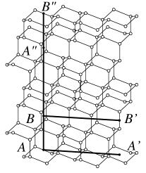
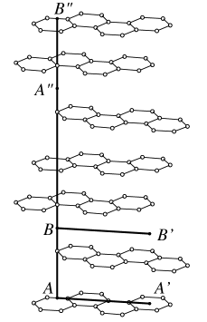
(a) diamond

(b) graphite

Figure 1: Crystal structure of (a) diamond and (b) rhombohedral graphite, illustrating stacked layers of hexagonally arranged carbon atoms for graphite and buckled layers for diamond. In both structures, the point $A$ lies at the midpoint of a carbon-carbon bond, with the lines $AA^{\prime}$ and $AA^{\prime\prime}$ extending within a layer and perpendicular to the layers, respectively. The point $B$ lies midway between two layers (at a hexagonal interstitial point in diamond) and the lines $BB^{\prime}$ and $BB^{\prime\prime}$ extend between the layers and perpendicular to the layers, respectively.

By this means we may plot inhomogeneous two-body functions in terms of the relative separation of the electrons in the system. In particular, we may draw some conclusions about electron correlation in the system by examination of $u$. We may determine the isotropy of $u$ by comparing plots of $u$ with the first electron kept at the same point but the second electron moved in perpendicular directions, e.g., by comparing plots designated by $AA^{\prime}$ and $AA^{\prime\prime}$. The homogeneity of $u$ may be seen by comparing plots of $u$ with the second electron moving in parallel directions from different positions of the first electron, e.g., by comparing $AA^{\prime}$ and $BB^{\prime}$. Any differences between these plots of $u$ are attributable to the inhomogeneity and anisotropy of the electron correlation factors in the systems studied.

We use periodic boundary conditions (PBC) to approximate the infinite crystal. Fahy et al. (1990a) The simulation cells consist of an $N_{1}\times N_{2}\times N_{3}$ unit cell arrangement. The unit cells in each system are defined by the Bravais lattice basis vectors. For diamond, we use the basis: $\{(a/2,a/2,0);\ (0,a/2,a/2);\ (a/2,0,a/2)\}$, where $a=6.72$ a.u., corresponding to a carbon bond-length of $2.91$ a.u. For rhombohedral graphite we use the basis: $\{(0,a,c);\ (-\sqrt{3}a/2,-a/2,c);\ (\sqrt{3}a/2,-a/2,c)\}$, where $a=2.68$ a.u. is the bond-length within the layers, and $c=6.33$ a.u. is the layer separation.

We construct the Slater determinant $D$ for both systems using DFT calculations in the local density approximation (LDA). Kohn and Sham (1965) The LDA orbitals were expanded using a linear combination of atomic orbitals comprising gaussians centred on each of the two carbon atoms in the unit cell. Fahy et al. (1990a); Malatesta et al. (1997); Chan et al. (1986)

IV.1 Removal of cusp

In Sec. II.1, we discussed the advantages of removing the short-range cusp from the function $u$ in order to improve its representability as a linear combination of smooth functions. Figure 2(a) compares the pseudointeraction $V_{\rm ps}$, generated using a cut-off radius of $r_{c}=1.9$ a.u. and energy eigenvalue $\epsilon=0.2$ hartree (as discussed in Ref. Prendergast et al., 2001), with the Coulomb interaction $V=e^{2}/r$. (In atomic units $e^{2}=1$). The pseudointeraction is used to generate a short-range Jastrow funtion $u_{\rm sr}$, which is shown in Fig. 2(b) for the relative angular momenta $l=1$ and $l=0$ corresponding to parallel spin and anti-parallel spin correlation, respectively. The short range Jastrow factor used in all subsequent calculations is that generated with these particular values of $r_{c}$ and $\epsilon$. Subsequent figures in this paper, which involve $u_{\rm sr}$, represent anti-parallel spin correlation only.

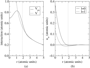
Figure 2: (a) The pseudo-interaction $V_{\rm ps}$ (solid line) and the Coulomb interaction $V=1/r$ (dashed line) versus electron separation $r$. (b) The short-range Jastrow function $u_{\rm sr}$, generated from $V_{\rm ps}$, versus electron separation $r$, for angular momenta $l=0$ (solid line) and $l=1$ (dashed line). $V_{\rm ps}$ is generated using $r_{c}=1.9$ a.u. (indicated by vertical dotted line) and $\epsilon=0.2$ hartree (see text).

The cut-off required for a convergent Fourier expansion of a smooth cuspless function should be much less than that required for a function with a short-range cusp. Therefore, using a cuspless form greatly reduces the number of terms required to represent the inhomogeneous form of the Jastrow factor accurately in Fourier space. We illustrate this point using a simple example. In Fig. 3 we plot $q^{2}$ times the Fourier transform, for wave vector $q$, of the Yukawa-style homogeneous correlation factor,

$$u_{\rm h}=\frac{A}{r}(1-e^{-r/F})~{},$$ (38)

which has been used by many authors to approximate electron correlation in a variety of systems. Fahy et al. (1990a); Filippi and Fahy (2000); Bevan (1997); Gaudoin et al. (2001); Malatesta et al. (1997); Ceperley (1978) We set $A=1$ a.u., ($F$ is determined from $A$ to satisfy the cusp conditions Kato (1957) and depends on the relative spin of the electrons). Also shown in Fig. 3 is $q^{2}$ times the Fourier transform of the cuspless difference $u_{\rm h}-u_{\rm sr}$. We assume that, for large electron separations, electron correlation is approximately spin-independent. Therefore, for each $q$, we plot the mean of the parallel spin and anti-parallel spin values of the functions.

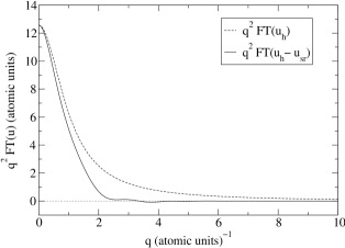
Figure 3: Fourier transform times $q^{2}$ of (a) the homogeneous Jastrow factor $u_{\rm h}$ (dashed line) and (b) the cuspless difference $u_{\rm h}-u_{\rm sr}$ (solid line) versus wave vector $q$. The homogeneous Jastrow factor parameter $A=1$ a.u. (Eq. 38).

In practice, we use the first zero of the Fourier transform of $V_{\rm ps}$ as the Fourier space cut-off $k_{c}$ used in the definition of $J_{\rm ih}$ in Eq. 15. For $r_{c}=1.9$ a.u. we use the cut-off $k_{c}=2.185~{}(\mbox{a.u.})^{-1}$, beyond which the Fourier transform of the cuspless $u$ function is approximately zero (Fig. 3). Combining both the short-range and inhomogeneous forms of the Jastrow factor using this scheme produces a form that is approximately independent of the cut-off, since decreasing $r_{c}$ increases the reciprocal space cut-off $k_{c}$.

IV.2 Homogeneous Jastrow Factor

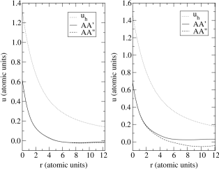
(a) diamond

(b) graphite

Figure 4: Jastrow correlation factors versus electron separation $r$ for (a) diamond and (b) rhombohedral graphite. (i) The function $u_{\rm h}$ (dotted line) as defined in Eq. 38 with optimized parameter $A=1.739$ for diamond and $2.170$ for graphite. (ii) The reconstructed function $u$ of Eq. 39, from a $3\times 3\times 3$ simulation region in both systems, for electron separations along the line segments $AA^{\prime}$ (solid line) and $AA^{\prime\prime}$ (dashed line) from Fig. 1.

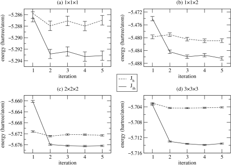
Figure 5: Energy of diamond, in hartree/atom, for each iteration of the optimization process and various simulation cell sizes using the inhomogeneous Jastrow factor $J_{\rm ih}$ (solid line): (a) $1\times 1\times 1$ unit cell, with $N=8$ electrons and $N_{\alpha}=140$ variational wave function parameters; (b) $1\times 1\times 2$, $N=16$, $N_{\alpha}=196$; (c) $2\times 2\times 2$, $N=64$, $N_{\alpha}=532$; (d) $3\times 3\times 3$, $N=216$, $N_{\alpha}=1235$. Also shown (dashed line) are energies during optimization of the one-body Jastrow factor $J_{\rm 1b}$ (with 84 variational parameters) in combination with the homogeneous Jastrow factor $J_{\rm h}$. Averages for each iteration are calculated using $10^{5}$ Monte Carlo samples.

For comparison with the inhomogeneous $u$ functions determined in the following sections we use the Yukawa-style homogeneous function $u_{\rm h}$ of Eq. 38 and construct a homogeneous trial wave function of the form $\Psi=J_{\rm sr}J_{\rm h}J_{\rm 1b}D$. As with the inhomogeneous trial wave function, we represent short-range correlation (i.e., the cusp) using $J_{\rm sr}$ and represent the remaining correlation using a homogeneous Jastrow factor

$$J_{\rm h}=\exp\left[-\sum_{q<k_{c}}\tilde{u}({\bf q})P_{\bf qq}\right]~{},$$

where we define

$$\tilde{u}({\bf q})\equiv\int_{\Omega}[u_{\rm h}(r)-u_{\rm sr}(r)]e^{-i{\bf q\cdot r}}d{\bf r}~{}.$$

For the uniform electron gas, Bohm and Pines Bohm and Pines (1953) predicted that the true function $u$ should decay as $1/\omega_{p}r$, at large separation $r$, where $\omega_{p}$ is the plasma frequency. Rather than use this limiting value $A=1/\omega_{p}$ in Eq. 38, it is common to treat $A$ as a free parameter such that the energy is minimized. Using variational calculations we can determine the optimal value of $A$. Malatesta et al. (1997) We optimize the one-body Jastrow factor $J_{\rm 1b}$ in Eq. 16, using our iterative method. The Jastrow factor $J=J_{\rm sr}J_{\rm h}J_{\rm 1b}$, combined with the Slater determinant $D$, is our best approximation of the true many-body eigenstate using a homogeneous two-body Jastrow factor and is comparable with similar wave functions optimized using variance minimization. Fahy et al. (1990a); Gaudoin et al. (2001); Malatesta et al. (1997)

In Fig. 4 we plot $u_{\rm h}$ and compare it with the reconstructed function

$$u({\bf r})=u_{\rm sr}(r)+\sum_{q<k_{c}}\tilde{u}({\bf q})e^{i{\bf q\cdot r}}~{},$$ (39)

for $3\times 3\times 3$ unit cell simulations of diamond and rhombohedral graphite. Periodic boundary conditions and the anisotropy of the unit cell make this reconstructed form appear quite different to the original isotropic function $u_{\rm h}$.

In particular, for rhombohedral graphite the unit cell used is quite anisotropic, leading to marked differences in the reconstructed function along the perpendicular line segments $AA^{\prime}$ and $AA^{\prime\prime}$. (The homogeneity of $u_{\rm h}$ is preserved and so we only plot the function for point $A$, since all other points are equivalent.) Note that the Jastrow $u$ function is defined up to an arbitrary constant, much like a potential, since this constant affects only the wave function normalization and contributes nothing to the description of correlation. Therefore, it is of no consequence that the functional form of $u_{\rm h}$ in Eq. 38 appears shifted above the reconstructed forms compatible with PBC. This is due to the removal of the constant Fourier coefficient of the correlation function $u({\bf G=0})$ from the expansion of the reconstructed function in Eq. 39. We note that the cusp conditions Kato (1957) are maintained by all forms.

We optimize the one-body Jastrow $J_{\rm 1b}$ using the method described in Sec. III. For the diamond simulations we used a Fourier space cut-off $G_{c}=5.0~{}\mbox{(a.u.)}^{-1}$, giving 84 variational one-body parameters. This is more than enough for an accurate representation of one-body terms in the wave function (see Sec. V.1). For graphite simulations we used $G_{c}=3.1~{}\mbox{(a.u.)}^{-1}$, giving 30 variational one-body parameters.

The values of the electronic energy per atom for various optimizations of this homogeneous trial wave function are shown in Figs. 5 and 6. Each iteration involved averaging over $10^{5}$ Monte Carlo samples. However, this amount of averaging was more than enough for an accurate implementation of the method. The optimization of the one-body terms in the $3\times 3\times 3$ simulation of graphite (Fig. 6) involved only $2.5\times 10^{4}$ samples per iteration and is well converged. On average, the gain in energy following one-body optimization is approximately $1.0$ mhartree/atom for diamond and $2.5$ mhartree/atom for graphite. We note that the necessity for a one-body correction is a consequence of the inhomogeneity of the electronic charge density in the system, Malatesta et al. (1997); Gaudoin et al. (2001) and it is not surprising that the gain in energy is larger for the more inhomogeneous system, graphite, than for diamond.

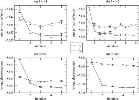
Figure 6: Energy of rhombohedral graphite, in hartree/atom, for each iteration of the optimization process and various simulation cell sizes using the inhomogeneous Jastrow factor $J_{\rm ih}$ (solid line): (a) $1\times 1\times 1$ unit cell, with $N=8$ electrons and $N_{\alpha}=162$ independent parameters for $J_{\rm ih}$; (b) $1\times 1\times 2$, $N=16$, $N_{\alpha}=272$; (c) $2\times 2\times 2$, $N=64$, $N_{\alpha}=1020$; (d) $3\times 3\times 3$, $N=216$, $N_{\alpha}=3136$. Also shown (dashed line) are energies during optimization of the one-body Jastrow factor $J_{\rm 1b}$ (with 30 variational parameters) in combination with the homogeneous Jastrow factor $J_{\rm h}$. Averages for each iteration are calculated using $10^{5}$ Monte Carlo samples. (The optimization of $J_{\rm 1b}$ for the $3\times 3\times 3$ simulation used only $2.5\times 10^{4}$ samples per iteration.)

The Slater determinant used in the diamond calculations of Fig. 5 is composed of single-particle orbitals generated from an LDA calculation. The LDA orbitals are linear combinations of gaussian basis functions of $s$, $p$ and $d$ symmetry, using three decays of 0.24, 0.797, and 2.65. The exchange-correlation functional used was of the Ceperley-Alder Ceperley and Alder (1980) form. The cut-off of the Fourier space expansion of the charge density Chan et al. (1986) in the LDA calculation was 64 Rydberg.

The graphite calculations shown in Fig. 6 use a Slater determinant generated using a gaussian basis-set with $s$ and $p$ symmetry only. Four decays were used: 0.19, 0.474, 1.183, and 2.95. The orbitals were generated from LDA calculations incorporating the Hedin-Lundqvist Hedin and Lundqvist (1971) exchange-correlation functional, and a cut-off of 36 Rydberg for the Fourier space expansion of the charge density. (See Sec. V.1 for a discussion of basis-set convergence of the total energy in graphite.)

Figure 7 illustrates the convergence during optimization of the one-body function $\chi({\bf r})$ in Eq. 1 (where $\chi$ is the accumulation of all one-body terms from each of the Jastrow factors) for the $3\times 3\times 3$ diamond calculation. The optimized function is statistically well-determined, and the change from the initial one-body function, $\chi^{1}=\chi^{0}$ of Eq. II.2 (as defined in Refs. Gaudoin et al., 2001 and Malatesta et al., 1997), is well-defined. This alteration of the one-body function may be compared to similar calculations performed using variance minimization. Malatesta et al. (1997); Gaudoin et al. (2001)

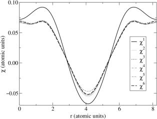
Figure 7: The diamond one-body function $\chi$ versus position $r$ along the line segment $AA^{\prime}$ [Fig. 1(a)]. $\chi^{n}$ indicates the one-body function used at iteration $n$ of the optimization of $J_{\rm 1b}$ in the presence of $J_{\rm h}$ in Fig. 5(d).

The number of parameters for optimization could be greatly reduced through exploitation of the crystal point-group symmetry of the structures involved. However, it is worth noting that the optimization process preserves the natural symmetry of the system (within statistical error) without such measures, illustrating that for non-symmetric systems with large numbers of parameters, this optimization process should be quite robust.

The one-body function $V^{n}({\bf r})$, reconstructed from the coefficients associated with the local energy $V_{\bf G}$ at iteration $n$ according to Eq. 36, is shown in Fig. 8. Clearly, this function decreases in magnitude, indicating a decrease in the magnitudes of the Euler-Lagrange derivatives. Beyond the first iteration, $V^{n}({\bf r})$ is of the same order of magnitude as its associated standard error, and so is statistically insignificant. Therefore, the method has essentially converged after only one iteration. The noisiest regions of $V^{n}({\bf r})$ correspond to regions of low density where the Monte Carlo sampling is less frequent.

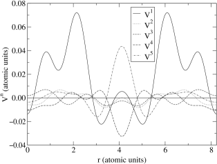
Figure 8: The reconstructed one-body function $V^{n}$, defined in Eq. 36, versus position $r$ as for Fig. 7.

IV.3 Inhomogeneous RPA Jastrow Factor

The analytic guess for the two-body predictor functions $S_{\bf qq^{\prime}}({\bf u})$, outlined in Sec. III.4.2, leads to an inhomogeneous generalization of the RPA equations. The solution to these equations is the function $u_{1}=u_{\rm RPA}$, shown in Fig. 9 for the $3\times 3\times 3$ graphite simulation. We notice some inhomogeneity in $u_{\rm RPA}$ at intermediate- and long-range electron separations. A more homogeneous and isotropic $u_{\rm RPA}$ was found for diamond, as we would expect since diamond possesses a more uniform electron density than graphite.

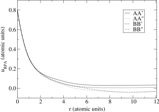
Figure 9: The Jastrow factor $u_{\rm RPA}$ versus electron separation $r$ along the line segments indicated in Fig. 1(b), for a $3\times 3\times 3$ simulation of rhombohedral graphite.

In Figs. 5 and 6, the first point on all solid curves indicates the total energy per atom in each simulation calculated using $u_{\rm RPA}$. In comparison with the energy calculated using the homogeneous Jastrow function $u_{\rm h}$, we see that the inhomogeneous RPA trial wave function is at best comparable in accuracy with the optimized trial wave function with homogeneous two-body Jastrow factor, and often less accurate. These results are different from those of Gaudoin et al. Gaudoin et al. (2001) for model systems: they find that their inhomogeneous generalization of the RPA produces wave functions that yield lower energies than the homogeneous form.

IV.4 Inhomogeneous Optimal Jastrow Factor

We simultaneously optimized the parameters in both the one-body Jastrow factor $J_{\rm 1b}$ and the fully inhomogeneous form of the two-body Jastrow factor $J_{\rm ih}$, using our iterative method. The convergence of the total energy per atom for various simulations of diamond and rhombohedral graphite are shown in Figs. 5 and 6. (The Slater determinants used in combination with the homogeneous Jastrow factor $J_{\rm h}$ in Sec. IV.2 are also used here.) Convergence of the total energy is achieved in approximately three iterations in all cases and is stable. This is remarkable given that the system sizes range from 8 electrons and 140 independent parameters to 216 electrons and 3136 independent parameters. Also, we used the same amount of Monte Carlo sampling, viz., $10^{5}$ samples per iteration, to determine the required expectation values for all simulations. In all cases the fully inhomogeneous form of $u$ allows us to determine more accurate trial wave functions with substantially lower energies than the homogeneous trial functions. In general, the gain in energy through using an inhomogeneous rather than a homogeneous wave function is of the order of $5$ mhartree/atom for both diamond and rhombohedral graphite.

Figure 10 illustrates the rapid convergence of the two-body wave function parameters ${\bf u}$ to their optimal values during the largest graphite optimization ($3\times 3\times 3$) and is typical of all the optimizations performed in both diamond and graphite. Beyond the third iteration, no clear distinction exists between subsequent sets of parameters. The optimal Jastrow function $u$ is significantly different from both the RPA function $u^{1}$ and the homogeneous form $u_{h}$ of Eq. 38. The proof that this optimization succeeds in minimizing the energy expectation value may be seen in Fig. 11 (which comes from the same graphite calculation as Fig. 10). Here, we plot the iterative decay of the two-body function $V^{n}({\bf r},{\bf r^{\prime}})$ reconstructed from the total energy coefficients determined at each iteration, according to Eq. IV. This clearly indicates the reduction to zero (within statistical noise) of the derivatives in the Euler-Lagrange equations, thus solving the energy minimization problem.

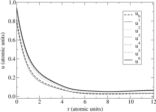
Figure 10: Graphite Jastrow correlation functions $u^{n}$ with respect to electron separation $r$ on the line segment $AA^{\prime}$ (Fig. 1) for each iteration $n$ during optimization of $J_{\rm ih}$ for a $3\times 3\times 3$ simulation region [Fig. 6(d)]. Also shown is the reconstruction of the homogeneous function $u_{h}$ (heavy dotted line) defined in Eq. 39 with optimized parameter $A=2.170$.

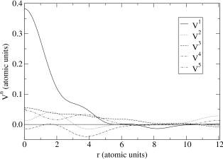
Figure 11: The reconstructed two-body function $V^{n}$, as defined in Eq. IV, versus electron separation $r$ on the line segment $AA^{\prime}$, for each iteration $n$ during the optimization outlined in Figs. 6(d) and 10.

For the largest simulation cells studied ($3\times 3\times 3$ unit cell arrangement containing 216 electrons), we compare the optimal Jastrow correlation functions $u$ of diamond and rhombohedral graphite. Figures 12 and 13 show the function $u$ plotted with respect to electron separation on various line segments in the corresponding crystal structures, as already explained.

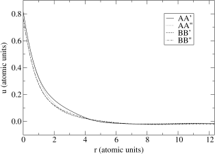
Figure 12: The optimized diamond Jastrow correlation factor $u$ as a function of electron separation $r$ along the line segments indicated, for a $3\times 3\times 3$ simulation region.

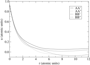
Figure 13: The optimized rhombohedral graphite Jastrow correlation factor $u$ as a function of electron separation $r$ along the line segments indicated, for a $3\times 3\times 3$ simulation region.

V Discussion

V.1 Energies

For a direct comparison of the calculated energies of diamond and rhombohedral graphite, we should (a) make some corrections based on the trial wave functions used and (b) include finite size and zero-point phonon energy corrections for the expected energy of the real infinite solid. The corrected energies for diamond and graphite are listed in Table 1.

Table 1: Energies and energy corrections of diamond and rhombohedral graphite (in hartree/atom). (a) Total energy, determined by VMC and our optimization method, for a $3\times 3\times 3$ unit cell simulation region, using wave functions of similar variational freedom (see text). (b) Finite size correction equal to the energy difference between an LDA calculation for the $3\times 3\times 3$ simulation region and an LDA calculation using a fully-converged k-point set (see text). (c) Correction for the zero-point phonon energy. Yin and Cohen (1984) (d) Total energy including the corrections. The numbers in parentheses indicate the statistical error in the last digits of the corresponding energy.

	diamond		graphite
$3\times 3\times 3$	$-5$.	712 95(14)	$-5$.	712 91(14)
finite size correction	$-0$.	008 99	$-0$.	006 56
zero-point energy	$0$.	006 65	$0$.	006 10
total	$-5$.	715 29(14)	$-5$.	713 41(14)

The Jastrow factors used in both solids are comparable in their variational freedom, the only significant difference being the size of the cut-off used for $\chi_{\rm 1b}$. However, a VMC calculation for diamond, using the same cut-off as in graphite ($G_{c}=3.1$ (a.u.)^-1, corresponding to 25 variational parameters), resulted in an increase in energy of only $1.0\pm 0.3$ mhartree/atom for diamond. Therefore, the high Fourier coefficients of $\chi_{\rm 1b}$ contribute little to the total energy of the system. The diamond VMC energy for the $3\times 3\times 3$ simulation quoted in Table 1 was determined using $G_{c}=3.1$ (a.u.)^-1 as the cut-off for one-body terms.

In graphite, the exclusion of $d$ symmetry from the basis set used to construct the LDA orbitals in the Slater determinant is energetically more important. In addition to the calculations described in Secs. IV.2 and IV.4, we also performed calculations for graphite using a gaussian basis set with $s$, $p$ and $d$ symmetry, and three gaussian decays: 0.22, 0.766, 2.67. For the $3\times 3\times 3$ simulation, including $d$ symmetry reduces the total VMC energy by $7.2\pm 0.3$ mhartree/atom and also reduces the variance in the total energy by 16%. Use of the Ceperley-Alder exchange correlation functional to generate the single-particle orbitals in graphite, rather than the Hedin-Lundqvist form, made no difference (within statistical error) to the VMC energies, and neither did an increase in the cut-off for the Fourier space expansion of the LDA charge density from 36 to 64 Rydberg. The graphite VMC energy for the $3\times 3\times 3$ simulation listed in Table 1 was calculated using a trial wave function very similar to that used for the calculation of the corresponding diamond VMC energy. The cut-off for the one-body Jastrow factor was $G_{c}=3.1$ (a.u.)^-1 and the Slater determinant comprised LDA orbitals obtained using: (i) a basis set with $d$ symmetry (as outlined above); (ii) the Ceperley-Alder exchange correlation functional; and (iii) a 64 Rydberg cut-off for the LDA charge density expansion.

We generate finite size corrections for the $3\times 3\times 3$ unit cell simulations of diamond and graphite, by calculating the difference in energy between an LDA calculation which uses k-points compatible with periodic boundary conditions of a $3\times 3\times 3$ simulation region and an LDA calculation using a fully converged k-point set. Fahy et al. (1990a) Comparing the change in energy between a $2\times 2\times 2$ calculation and a $3\times 3\times 3$ calculation in both diamond and graphite, using LDA and VMC, we see that the change in VMC energy is about 80% of the LDA energy change in diamond, and 70% in rhombohedral graphite. Perhaps more accurate estimates of the energy of the infinite solid may be obtained by implementation of a model periodic Coulomb interaction developed recently. Tests of this approach have dramatically reduced finite-size effects in the interaction energy. Fraser et al. (1996); Williamson et al. (1997); Kent et al. (1999)

For diamond, we estimated the finite size correction to be $-8.99$ mhartree/atom, using a converged LDA calculation with 220 k-points in the irreducible Brillouin zone. For rhombohedral graphite, incorporating $d$ symmetry in the basis set (as described above), and using 189 k-points in the LDA calculation, we found the finite size correction to be $-6.56$ mhartree/atom. We also include the calculated zero-point phonon energies of diamond and graphite, which are $6.65$ and $6.10$ mhartree/atom, respectively. Yin and Cohen (1984)

Adding all these corrections to the calculated VMC energies (Table 1), we estimate the energies of the infinite solids to be $-5.71529\pm 0.00014$ hartree/atom for diamond and $-5.71341\pm 0.00014$ hartree/atom for rhombohedral graphite. This appears to indicate that rhombohedral graphite is less stable than diamond. However, given the approximation of using LDA finite size corrections, we might expect a systematic error of the order of 2 mhartree/atom in each of these results. This indicates that at the VMC level, the solids diamond and rhombohedral graphite have very similar total energies. We note that in the atomic pseudopotential used in the calculations presented here $p$ and higher angular momentum scattering are all included in the local potential. It is possible that the use of a separate $d$ pseudopotential might slightly affect the relative energies in both systems.

In order to determine the cohesive energy of a solid, we should subtract the energy per atom of the solid from the energy of the isolated atom, $E_{c}=E_{a}-E_{s}$. However, when using approximate eigenfunctions, a reasonable estimate of the cohesive energy is obtainable only by subtracting the energies estimated using similar trial wave functions. VMC energies are available for the carbon atom where the trial wave function is of the Jastrow-Slater form. Filippi and Fahy (2000) The orbitals of the Slater determinant are optimized using energy minimization and a sophisticated Jastrow factor is optimized using variance minimization, yielding a VMC energy for the atom of $-5.4372\pm 0.0001$ mhartree. Using this energy, we find the cohesive energies to be $0.2781\pm 0.0002$ hartree/atom for diamond and $0.2762\pm 0.0002$ hartree/atom for graphite. We regard this atomic trial wave function to be close in form and accuracy to our solid trial wave function. However, to remain consistent with the inclusion of $d$ symmetry in the basis set of our LDA calculations, we could also refer to a multiconfiguration trial wave function for the carbon atom which includes $d$ excitations. The VMC energy of the atom, using this wave function, is $-5.45061\pm 0.00002$ hartree, Filippi and Fahy (2000) leading to estimates of the cohesive energies of diamond and rhombohedral graphite of $0.2647\pm 0.0002$ hartree/atom and $0.2628\pm 0.0002$ hartree/atom, respectively. The experimental values are 0.271 hartree/atom for diamond, and 0.272 hartree/atom for graphite. Brewer

Considering the significant gain in energy obtained using an inhomogeneous Jastrow factor rather than a homogeneous form, one might wonder how much the difference between VMC and DMC energies has been reduced. Using Jastrow correlation factors which include one-body terms and homogeneous two-body terms, similar in form to that used in Sec. IV.2, for bulk carbon Kent and silicon, Li et al. (1991) typically leads to VMC correlation energies that are approximately 90% of the corresponding DMC correlation energies, i.e.,

$$\frac{E_{\rm VMC}-E_{\rm HF}}{E_{\rm DMC}-E_{\rm HF}}\approx 0.90~{},$$

where $E_{\rm VMC}$ is the energy calculated using VMC, $E_{\rm DMC}$ is the energy calculated using DMC, and $E_{\rm HF}$ is the Hartree-Fock energy. ($E_{\rm HF}$ has been estimated using just the LDA Slater determinant as trial wave function. Fahy et al. (1990a)) We have observed that including inhomogeneity in the correlation factor leads to a gain in energy of approximately 10 mhartree/atom in the largest simulations of both diamond and graphite. If we estimate that the VMC correlation energy, determined using our optimized wave function with homogeneous correlation terms, obtains 90% of $E_{\rm DMC}-E_{\rm HF}$, then using the optimized wave function with inhomogeneous correlation terms obtains 96% of the DMC correlation energy. This would indicate that the energy difference between VMC and DMC for these solids has been decreased by 60%.

It is important to emphasize that, whatever physical conclusions we would like to draw from these calculations, our principal aim has been to optimize the trial wave function for a given Hamiltonian, such that the expectation value of the total energy is minimized. This aim has been achieved for all the systems studied.

V.2 Correlation Factors

Diamond, with a relatively homogeneous and isotropic electron charge density, exhibits an approximately homogeneous, isotropic Jastrow correlation function $u$ (Fig. 12). At large electron separations (beyond 6 a.u.) we see that the electron correlation factor $u$ in diamond is well approximated by homogeneous and isotropic functions, as all the curves plotted are quite similar. Only slight deviations from homogeneity exist at short and intermediate electron separations. This inhomogeneity may be seen by comparing $u$ plotted with its fixed coordinate at different points: $AA^{\prime}$ and $AA^{\prime\prime}$ are quite similar at short range, but clearly distinct from $BB^{\prime}$ and $BB^{\prime\prime}$ in the same region. This inhomogeneity may have significant effects on the short-range pair-correlation functions calculated for diamond-like systems using VMC methods. Fahy et al. (1990b); Hood et al. (1997, 1998)

Graphite, with clear regions of high electron charge density and well-defined regions of very low electron charge density between its layers, is a highly inhomogeneous and anisotropic structure. This is borne out in Fig. 13, where the function $u$ differs considerably in various regions and in various directions. At short-range, $u$ is surprisingly homogeneous in comparison with diamond. At intermediate separations the function displays both inhomogeneous and anisotropic behaviour. Given that the layer separation in these simulations is 6.33 a.u., this indicates that inhomogeneous correlation between adjacent layers in the system is not insignificant. This may prove important for van der Waals interactions between the layers in graphite.

At long range, the anisotropy of the graphite correlation factor is clearly shown in Fig. 13, where the correlation factors for electron separation vectors ${\bf r^{\prime}-r}$ lying parallel to the graphite planes ($AA^{\prime}$ and $BB^{\prime}$) are distinctly different from those with the separation vector perpendicular to the planes ($AA^{\prime\prime}$ and $BB^{\prime\prime}$). Inhomogeneity (i.e. an explicit dependence on the position ${\bf r}$ of the first electron) is displayed at long range in the differences between the function along $AA^{\prime}$ and $BB^{\prime}$. We might expect this, given that the line AA’ lies within the graphite planes, where the charge density is concentrated, whereas $BB^{\prime}$ lies in the very low charge density region between the planes [see Fig. 1(b)]. On the other hand, when the separation vector is oriented perpendicular to the graphite planes ($AA^{\prime\prime}$ and $BB^{\prime\prime}$), inhomogeneous effects are substantially smaller at long range.

V.3 Computational Details

In order to reduce the complexity of the physical results in Sec. IV, some computational details of the method were not discussed. We present and discuss some of these details in this section.

(1) This iterative method is trivially parallelizable. To determine the expectation values required to construct the predictor, Monte Carlo sampling may be performed independently on many workstations and the results combined. To obtain total energies of the accuracy presented in this paper requires $\sim 10^{5}$ Monte Carlo samples. However, for optimization of the wave function using our method, this amount of sampling is also sufficient for accurate estimations of the expectation values required to construct the predictor (Sec. III.5).

The extra time required to accumulate the various contributions to the predictor represents less than $5\%$ of the computational time needed to calculate each energy sample. There are two reasons for this: Firstly, because we have expressed the variational components of the Jastrow factor as linear combinations of the operators ${\cal O}_{m}$ of Sec. III. These ${\cal O}_{m}$ need only be evaluated once, for each electron configuration, in order to construct both the Jastrow factor and the predictor. Secondly, and more importantly, since we must calculate the total energy as a sum of various contributions defined by the Hamiltonian of the system, all the energy contributions needed to construct the predictor are already available, either directly or by some simple manipulation. It is also important to note that, despite the complex form of the Jastrow factor outlined in Sec. II, the amount of computational time spent evaluating it is still less than or equal to that spent evaluating the Slater determinant, for a given electron configuration.

The largest calculations presented in this paper were performed on a Beowulf cluster of fifteen 500 MHz dual-processor workstations. For a 5 iteration optimization using $10^{5}$ samples per iteration, these calculations took about 50 hours on this cluster. However, perhaps half this amount of sampling would have produced comparable results [see (3) below]. The required memory for storing all the expectation values necessary for this calculation was approximately 20 MB.

(2) The Newton-Raphson method (see Appendix C), while quadratically convergent near a root of a multidimensional system, does possess some convergence problems far from the root. In the calculations presented in this paper, we found that below a certain minimum amount of sampling, the noise in the estimated expectation values used to construct the predictor caused divergence of the solution to Eq. 33 using the Newton-Raphson method. This problem might be solved through the use of a more robust root-finding method for the predictor function.

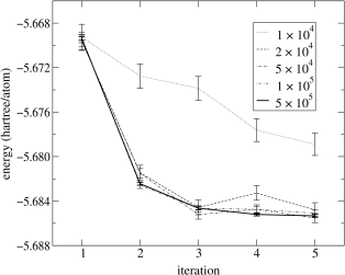
Figure 14: Total graphite energy in hartree/atom versus iteration number for a $2\times 2\times 2$ simulation region. The number of Monte Carlo samples per iteration ranges from $10^{4}$ to $5\times 10^{5}$.

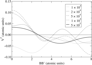
Figure 15: The reconstructed two-body function $V^{5}$, versus electron separation $r$ along the line segment $BB^{\prime}$ in graphite, from the fifth iteration of each of the calculations in Fig. 14.

(3) From the analysis in Appendix G, we see that noise in the iterative method comes from the finite sampling used to estimate those expectation values (listed in Sec. III.5) required to construct the predictor. The effect of this noise on the wave function accuracy is not clear. To reduce the computational cost of these calculations we would prefer to do the least amount of sampling necessary to produce the required results.

Figure 14 illustrates the effect of various amounts of sampling on the convergence of the total energy in the optimization of the $2\times 2\times 2$ simulation of rhombohedral graphite. At $10^{4}$ samples per iteration, the estimation of the required expectation values, during the first iteration of our method, is too crude to produce a convergent root of the predictor using the Newton-Raphson method. This leads to a wave function, used in the second iteration, with many noisy parameters which are more difficult to optimize, as the convergence of the energy shows. However, for sampling involving $2\times 10^{4}$ samples per iteration, or more, we see that the convergence of the total energy is identical (within statistical accuracy). Comparison of the optimized wave function parameters also reveals only small differences, indicating that the only means of determining the true benefits of more sampling is by examination of the fitted coefficients $V_{m}(\mbox{\boldmath$\alpha$}^{n})$ at each iteration $n$.

In Fig. 15 we see, from the reconstruction $V^{5}({\bf r},{\bf r^{\prime}})$ of the fitted coefficients for two-body optimization at the fifth and final iteration of the method, that the most sampling ($5\times 10^{5}$ samples per iteration) reduces the magnitude of the Euler-Lagrange derivatives the most, indicating that these wave function parameters are the most accurate. However, for practical purposes, there is little distinction between the accuracy of the wave function once we increase the sampling beyond $2\times 10^{4}$ samples per iteration. Thus, the optimizations presented in Sec. IV may have used more computational time than was strictly necessary. However, more testing is required to determine the minimum amount of sampling as a function of system size.

VI Conclusion

We have developed a generalized form of electron correlation factor for trial many-body wave functions of electrons in periodic solids. This form allows us to represent fully inhomogeneous electron correlation in real physical periodic systems. It is computationally efficient to evaluate, since the electron cusp, which we express as a homogeneous correlation factor, is separated from the fully inhomogeneous form.

We have also developed a rapidly convergent iterative method for the optimization of all variational parameters in these wave functions, minimizing the total energy of the given system. It uses the accurate techniques of quantum Monte Carlo sampling to achieve this optimization and has allowed new insights into the form of many-electron correlation in systems with highly inhomogeneous charge densities. We estimate the difference in energies calculated using the optimal inhomogeneous two-body correlation factor and the optimal homogeneous correlation factor to be approximately 60% of the difference between the DMC and VMC energies obtained with homogeneous 2-body correlation terms.

In diamond, the optimal correlation factor is approximately homogeneous and isotropic, with some inhomogeneity at short- and intermediate-range electron separations. This is consistent with its comparatively homogeneous and isotropic electron charge density. Graphite has an optimal correlation factor which is quite homogeneous at short-range electron separation, but is significantly inhomogeneous and anisotropic at intermediate- and long-range electron separations, as one might expect from its highly inhomogeneous and anisotropic electron charge density. Nevertheless, it is remarkable that despite very large inhomogeneity in the electron pair-correlation function, found by previous authors, Fahy et al. (1990b); Hood et al. (1997, 1998) the ideal inhomogeneous Jastrow two-body term, calculated for the first time here for diamond and graphite, displays relatively small inhomogeneity. Whether this conclusion can be extended to other systems (e.g. involving strongly correlated $d$-electrons) remains an open question.

Appendix A Derivative of observables with respect to wave function parameters

The derivative of the expectation value of an observable $A$, with respect to a parameter $\alpha_{m}\in\mbox{\boldmath$\alpha$}$ of the parameterized wave function $\Psi(\mbox{\boldmath$\alpha$})$, may be written as

$$\frac{\partial\langle A\rangle}{\partial\alpha_{m}}=\frac{\partial}{\partial\alpha_{m}}\frac{\langle\Psi|A|\Psi\rangle}{\langle\Psi|\Psi\rangle}.$$

We assume that $A$ is independent of the parameters $\alpha$. Also, for a time independent system, we may in general express $\Psi$ as a real function. Differentiating, we find that

$$\frac{\partial}{\partial\alpha_{m}}\langle\Psi|\Psi\rangle = 2\langle\Psi|{\cal O}_{m}|\Psi\rangle$$

$$\frac{\partial}{\partial\alpha_{m}}\langle\Psi|A|\Psi\rangle = 2\langle\Psi|A{\cal O}_{m}|\Psi\rangle$$

where we define the operator associated with variations of $\alpha_{m}$ as ${\cal O}_{m}\equiv\partial/\partial\alpha_{m}$, with local value

$${\cal O}_{m}({\bf R})\equiv\frac{1}{\Psi({\bf R})}\frac{\partial\Psi({\bf R})}{\partial\alpha_{m}}=\frac{\partial}{\partial\alpha_{m}}\ln\Psi({\bf R})~{},$$

for the many-body configuration ${\bf R}$.

Therefore, we may express the derivative of $\langle A\rangle$ as

$$\frac{1}{2}\frac{\partial\langle A\rangle}{\partial\alpha_{m}} = \frac{\langle\Psi|A{\cal O}_{m}|\Psi\rangle}{\langle\Psi|\Psi\rangle}-\frac{\langle\Psi|A|\Psi\rangle}{\langle\Psi|\Psi\rangle}\frac{\langle\Psi|{\cal O}_{m}|\Psi\rangle}{\langle\Psi|\Psi\rangle}$$

$$= \langle A{\cal O}_{m}\rangle-\langle A\rangle\langle{\cal O}_{m}\rangle$$

$$= \langle\Delta\!A\Delta\!{\cal O}_{m}\rangle,$$

where $\Delta\!A({\bf R})=A({\bf R})-\langle A\rangle$ and $\Delta\!{\cal O}_{m}({\bf R})={\cal O}_{m}({\bf R})-\langle{\cal O}_{m}\rangle$.

Appendix B Least-squares fitting

Our task is to minimize the integral

$$\chi^{2}=\langle\Psi|\left\{{\cal H}-E_{0}-\sum_{k}V_{k}{\cal O}_{k}\right\}^{2}|\Psi\rangle$$

by choosing the appropriate parameters $E_{0}$ and $\{V_{k}\}$. We note first that, at the minimum,

$$E_{0}=\langle E\rangle-\sum_{k}V_{k}\langle{\cal O}_{k}\rangle\ ,$$

where $\langle E\rangle$ is the expectation value of the total energy and $\langle{\cal O}_{k}\rangle$ is the expectation value of the operator ${\cal O}_{k}$. To fulfill the minimization, we must set all the remaining first derivatives of $\chi^{2}$ to zero, i.e.,

$$\frac{\partial\chi^{2}}{\partial V_{l}}=-2\langle\Psi|\left\{{\cal H}-E_{0}-\sum_{k}V_{k}{\cal O}_{k}\right\}{\cal O}_{l}|\Psi\rangle=0\ .$$

for each $l$. Upon substitution of the minimum value of $E_{0}$, this leads to

$$\langle E\,{\cal O}_{l}\rangle-\langle E\rangle\langle{\cal O}_{l}\rangle=\sum_{k}V_{k}[\langle{\cal O}_{k}{\cal O}_{l}\rangle-\langle{\cal O}_{k}\rangle\langle{\cal O}_{l}\rangle]\ .$$

Since, for any operators ${a}$, ${b}$ we may say that

$$\langle a\,b\,\rangle-\langle a\rangle\langle b\,\rangle=\langle\Delta a\,\Delta b\,\rangle$$

where $\Delta a=a-\langle a\rangle$, then we are lead to the conclusion that the least squares fitting is equivalent to solving the linear system

$$\sum_{k}V_{k}\langle\Delta{\cal O}_{k}\,\Delta{\cal O}_{l}\rangle=\langle\Delta E\,\Delta{\cal O}_{l}\rangle$$

for each $l$.

Appendix C Newton-Raphson Method

An integral part of the iterative procedure outlined in Sec. III.2 is the determination of the parameters $\alpha$ that solve the system in Eq. 33. The determination of the roots of any multidimensional function can be troublesome. In all the optimizations presented in this paper, the predictor function $V^{\prime}_{m}(\mbox{\boldmath$\alpha$};\mbox{\boldmath$\alpha$}^{0})$ is a quadratic function of $\alpha$, whose coefficients are determined analytically, or by numerical fitting at the point $\mbox{\boldmath$\alpha$}^{0}$. We ignore the implicit dependence of $V^{\prime}_{m}$ on $\mbox{\boldmath$\alpha$}^{0}$ for the purpose of finding a root, and solve the system $V^{\prime}_{m}(\mbox{\boldmath$\alpha$})=0$ for all $m$.

We use the Newton-Raphson method Press et al. (1990) to determine the roots. This is an iterative method of improving successive guesses for a root of a function. It involves the computation of the function $V^{\prime}_{m}$ and its Jacobian matrix of derivatives with respect to $\alpha$, at each guess. The iterations continue until convergence of the solution is achieved within a predefined tolerance.

The success of the Newton-Raphson method for multi-dimensional systems relies heavily on the proximity of the initial guess to the root we seek. For this reason, the initial guess chosen is normally the parameter set of the previous iteration of the procedure outlined in Sec. III.2. To find the first set of parameters, by finding the roots of the analytic predictor $S_{m}$, we require a good initial guess of the root. Since the one-body parameters $\chi_{\bf G}$ are expected to be small by construction, an initial guess of zero for all ${\bf G}$ was found to be sufficient to produce a convergent solution to the first application of the Newton-Raphson method.

For the two-body problem, we rescale the variables $u_{\bf qq^{\prime}}$ to improve the convergence of the root-finding method. According to the RPA, Bohm and Pines (1953) the long-range behaviour of the $u$ function should take the form $u(r)=1/\omega_{p}r$, where the plasma frequency for a homogeneous system with electron charge density $n$ is $\omega_{p}=\sqrt{4\pi n}$. The charge density $n$ is determined in the simulation region to be $N/\Omega$, for $N$ the number of electrons in the simulation volume $\Omega$. Therefore, for small ${\bf q}$ in Fourier space, $u$ behaves like

$$u({\bf q})=\frac{4\pi}{\Omega\omega_{p}q^{2}}=\omega_{p}\frac{1}{Nq^{2}}~{}.$$

This indicates large relative differences between values of $u({\bf q})$ for small ${\bf q}$. Therefore, in inhomogeneous systems, it would be appropriate to rescale the parameters $u_{\bf qq^{\prime}}$ by multiplying by $N|{\bf q}||{\bf q^{\prime}}|$, thus rendering all the variables of the same order of magnitude as the plasma frequency. This leads to a less pathological numerical problem for the Newton-Raphson method. Appropriate scaling must also be applied to the predictor function $V^{\prime}_{\bf qq^{\prime}}$ in Sec. III. For the initial analytic guess of the roots of $S_{\bf qq^{\prime}}$ we use the homogeneous solution for $u_{\bf qq^{\prime}}$ outlined in Eq. 34.

Appendix D One-body Energy Contributions

The variational part of $\Psi$ associated with one-body terms is the Jastrow factor $J_{\rm 1b}$ (Eq. 16) with parameters $\mbox{\boldmath$\chi$}=\{\chi_{\bf G}\}$. We expand the energy contributions $\epsilon^{(1)}$ and $\epsilon^{(2)}$ defined in Sec. III.3. For $J_{\rm 1b}$, we have that

$$\epsilon^{(1)} \equiv -\frac{1}{2}\sum_{i}\frac{\nabla_{i}^{2}J_{\rm 1b}}{J_{\rm 1b}}$$

$$= -\frac{1}{2}\sum_{i}(\nabla_{i}^{2}\ln J_{\rm 1b}+|\mbox{\boldmath$\nabla$}_{i}\ln J_{\rm 1b}|^{2})$$

$$= \frac{1}{2}\sum_{\bf G}\chi_{\bf G}G^{2}\Delta\rho_{\bf G}^{*}$$

$$+\frac{1}{2}\sum_{\bf GG^{\prime}}\chi_{\bf G-G^{\prime}}({\bf G-G^{\prime}}){\bf\cdot G^{\prime}}\chi_{\bf G^{\prime}}\Delta\rho_{\bf G}^{*}+\mbox{constant}~{}.$$

The constant terms are not required, so we ignore them.

The energy contribution $\epsilon^{(2)}$ cannot be expanded analytically as a linear combination of the functions $\Delta\rho_{\bf G}^{*}$ since $\Psi^{\prime}\equiv\Psi/J_{\rm 1b}$ is not explicitly a function of these coordinates.

$$\epsilon^{(2)} \equiv -\sum_{i}\frac{\mbox{\boldmath$\nabla$}_{i}J_{\rm 1b}}{J_{\rm 1b}}\mbox{\boldmath$\cdot$}\frac{\mbox{\boldmath$\nabla$}_{i}\Psi^{\prime}}{\Psi^{\prime}}$$

$$= -\sum_{\bf G}\chi_{\bf G}\sum_{i}\mbox{\boldmath$\nabla$}_{i}\Delta\!\rho_{\bf G}^{*}\mbox{\boldmath$\cdot$}\frac{\mbox{\boldmath$\nabla$}_{i}\Psi^{\prime}}{\Psi^{\prime}}$$

However, $\epsilon^{(2)}$ is explicitly linear in the parameters $\chi$, with derivatives

$$\frac{\partial\epsilon^{(2)}}{\partial\chi_{\bf G}}=-\sum_{i}\mbox{\boldmath$\nabla$}_{i}\Delta\!\rho_{\bf G}^{*}\mbox{\boldmath$\cdot$}\frac{\mbox{\boldmath$\nabla$}_{i}\Psi^{\prime}}{\Psi^{\prime}}~{},$$

which are independent of $\chi$.

Appendix E Two-body Energy Contributions

The variational part of $\Psi$ associated with two-body energy contributions is the inhomogeneous Jastrow factor $J_{\rm ih}$ of Eq. 15, with parameters ${\bf u}=\{u_{\bf qq^{\prime}}\}$. (For periodic systems we use only $u_{{\bf q+G},{\bf q+G^{\prime}}}$.) The energy contributions $\epsilon^{(i)}$ of Sec. III.3 are expanded here. The contribution $\epsilon^{(1)}$ is dependent only on the form of $J_{\rm ih}$ and is expanded as

$$\epsilon^{(1)}\equiv-\frac{1}{2}\sum_{i}\frac{\nabla_{i}^{2}J_{\rm ih}}{J_{\rm ih}}=-\frac{1}{2}\sum_{i}(\nabla_{i}^{2}\ln J_{\rm ih}+|\mbox{\boldmath$\nabla$}_{i}\ln J_{\rm ih}|^{2})~{}.$$

We find that

$$-\frac{1}{2}\sum_{i}\nabla_{i}^{2}\ln J_{\rm ih}=-\frac{1}{2}\sum_{\bf qq^{\prime}}u_{\bf qq^{\prime}}(q^{2}+q^{\prime 2})P_{\bf qq^{\prime}}$$

$$-\sum_{\bf q}\left[\frac{N-1}{N}\sum_{\bf q^{\prime}}u_{\bf qq^{\prime}}q^{2}\langle\rho_{\bf q^{\prime}}\rangle\right]\Delta\rho_{\bf q}^{*}+\mbox{constant}~{}.$$

We retain only the linear combination of the functions $P_{\bf qq^{\prime}}$. The constant terms we may ignore, and the one-body terms (linear combinations of $\Delta\rho_{\bf q}^{*}$) we assume are compensated by terms in the one-body Jastrow $J_{\rm 1b}$.

If we ignore the removal of one-body terms from the function $P_{\bf qq^{\prime}}=(\Delta\rho_{\bf q}^{\mbox{}}\Delta\rho_{\bf q^{\prime}}^{*})_{[i\neq j]}$ and consider using the function $\Delta\rho_{\bf q}^{\mbox{}}\Delta\rho_{\bf q^{\prime}}^{*}$ instead, then we find that

$$-\frac{1}{2}\sum_{i}|\mbox{\boldmath$\nabla$}_{i}\ln J_{\rm ih}|^{2}=$$

$$-2\sum_{\bf qq^{\prime}}\sum_{\bf kk^{\prime}}u_{\bf qk}({\bf k\cdot k^{\prime}})u_{\bf k^{\prime}q^{\prime}}\rho_{\bf k^{\prime}-k}\Delta\rho_{\bf q}^{\mbox{}}\Delta\rho_{\bf q^{\prime}}^{*}+\cdots~{},$$

where we have ignored constant and one-body terms in the expansion. The product $\rho_{\bf k^{\prime}-k}\Delta\rho_{\bf q}^{\mbox{}}\Delta\rho_{\bf q^{\prime}}^{*}$ contains both two- and three-body terms, since we may rewrite $\rho_{\bf k^{\prime}-k}$ as $\Delta\rho_{\bf k^{\prime}-k}+\langle\rho_{\bf k^{\prime}-k}\rangle$. We intend here to remove two-body fluctuations and regard three-body fluctuations as much less significant, so we retain only the two-body term  $\langle\rho_{\bf k^{\prime}-k}\rangle\Delta\rho_{\bf q}^{\mbox{}}\Delta\rho_{\bf q^{\prime}}^{*}$ from the charge fluctuation products in Eq. E, i.e.,

$$-2\sum_{\bf qq^{\prime}}\sum_{\bf kk^{\prime}}u_{\bf qk}({\bf k\cdot k^{\prime}})u_{\bf k^{\prime}q^{\prime}}\langle\rho_{\bf k^{\prime}-k}\rangle\Delta\rho_{\bf q}^{\mbox{}}\Delta\rho_{\bf q^{\prime}}^{*}+\cdots~{}.$$

Now we make the assumption that removing one-body terms from this expression , i.e., replacing $\Delta\rho_{\bf q}^{\mbox{}}\Delta\rho_{\bf q^{\prime}}^{*}$ with $P_{\bf qq^{\prime}}$ is a good approximation, and obtain the expression for $v_{\bf qq^{\prime}}^{(1)}({\bf u})$ given in Sec. III.4.2.

The contribution $\epsilon^{(2)}$ cannot be expanded analytically in the basis of fluctuation functions $P_{\bf qq^{\prime}}$, However, it is clear that $\epsilon^{(2)}$ is linear in ${\bf u}$, since, for $\Psi^{\prime}\equiv\Psi/J_{\rm ih}$,

$$\epsilon^{(2)}=\sum_{\bf qq^{\prime}}u_{\bf qq^{\prime}}\sum_{i}{\bf\nabla}_{i}P_{\bf qq^{\prime}}{\bf\cdot}\frac{{\bf\nabla}_{i}\Psi^{\prime}}{\Psi^{\prime}}~{},$$

and has first derivatives

$$\frac{\partial\epsilon^{(2)}}{\partial u_{\bf qq^{\prime}}}=\sum_{i}{\bf\nabla}_{i}P_{\bf qq^{\prime}}{\bf\cdot}\frac{{\bf\nabla}_{i}\Psi^{\prime}}{\Psi^{\prime}}~{}.$$

which are independent of the parameters ${\bf u}$.

The final energy contribution $\epsilon^{(3)}$ we attempt to express analytically in terms of the two-body fluctuation functions $P_{\bf qq^{\prime}}$. If $\Psi^{\prime}\approx D$, the LDA Slater determinant, then the sum of contributions from the external potential and the kinetic energy term $-(1/2)\sum_{i}\nabla_{i}^{2}\Psi^{\prime}/\Psi^{\prime}$ is a one-body contribution defined by the Kohn-Sham Hamiltonian, Kohn and Sham (1965) since

$$\sum_{i}[-\frac{1}{2}\frac{\nabla_{i}^{2}D}{D}+V_{\rm ext}({\bf r}_{i})]=\sum_{i}[\epsilon^{\rm KS}_{i}-V_{\rm H}({\bf r}_{i})-V_{\rm xc}({\bf r}_{i})]~{},$$

where $\epsilon^{\rm KS}_{i}$ are the Kohn-Sham eigenvalues, $V_{\rm H}$ is the Hartree potential and $V_{\rm xc}$ is the exchange and correlation potential. Therefore, the two-body contribution of these terms is approximately zero. We are left with the contribution of the electron-electron interaction $V$.

For a two-body potential $V({\bf r},{\bf r^{\prime}})$, we may expand the sum over electron pairs as

$$\sum_{i<j}V({\bf r}_{i},{\bf r}_{j}) = \frac{1}{2}\sum_{\bf qq^{\prime}}V_{\bf qq^{\prime}}\sum_{i\neq j}e^{-i{\bf q\cdot r}_{i}}e^{i{\bf q^{\prime}\cdot r}_{j}}$$

$$= \frac{1}{2}\sum_{\bf q}V_{\bf qq^{\prime}}(\rho_{\bf q}\rho_{\bf q^{\prime}}^{*})_{[i\neq j]}~{},$$

for Fourier coefficients $V_{\bf qq^{\prime}}$. In terms of the fluctuation functions $P_{\bf qq^{\prime}}$, this may be rewritten as

$$\sum_{i<j}V({\bf r}_{i},{\bf r}_{j})=\frac{1}{2}\sum_{\bf qq^{\prime}}V_{\bf qq^{\prime}}P_{\bf qq^{\prime}}$$

$$-\sum_{\bf q}\left[\frac{N-1}{N}\sum_{\bf q^{\prime}}V_{\bf qq^{\prime}}\langle\rho_{\bf q^{\prime}}\rangle\right]\Delta\rho_{\bf q}^{*}+~{}\mbox{constant}~{}.$$

(We assume that $V({\bf r},{\bf r^{\prime}})$ possesses exchange symmetry, so that $V_{\bf qq^{\prime}}=V_{\bf-q^{\prime}-q}$.) Therefore, both one- and two-body fluctuations arise from a two-body potential in the “charge fluctuation” coordinate system. Note that the one-body fluctuations are expressible in terms of the Hartree potential, since

$$V_{\rm H}({\bf q})=\sum_{\bf q^{\prime}}V_{\bf qq^{\prime}}\langle\rho_{\bf q^{\prime}}\rangle~{}.$$

If the two-body potential is homogeneous, i.e. $V({\bf r},{\bf r^{\prime}})=V({\bf r-r^{\prime}})$, then we may simplify the fluctuations since $V_{\bf qq^{\prime}}=V_{\bf q}^{*}\delta({\bf q-q^{\prime}})$, where the Fourier transform of the homogeneous function $V({\bf r})$ is

$$V_{\bf q}\equiv\frac{1}{\Omega}\int_{\Omega}V({\bf r})e^{-i{\bf q\cdot r}}d{\bf r}~{},$$

for a system volume $\Omega$. If $V({\bf r})=V(-{\bf r})$ then $V_{\bf q}^{*}=V_{\bf q}$. Therefore,

$$\sum_{i<j}V(|{\bf r}_{i}-{\bf r}_{j}|) = \frac{1}{2}\sum_{\bf q}V_{\bf q}P_{\bf qq}$$

$$- \frac{N-1}{N}\sum_{\bf q}V_{\bf q}\langle\rho_{\bf q}\rangle\Delta\rho_{\bf q}^{*}+~{}\mbox{constant}~{}.$$

Again we ignore the one-body and constant terms in this context.

Appendix F Consequences of using the short-range Jastrow

The short range Jastrow factor $J_{\rm sr}$ is constructed from the pseudointeraction $V_{\rm ps}$ in the following way. For the isolated two-electron scattering problem, we may find an eigenstate $\psi_{0}$ of the true two-electron Hamilatonian $h_{0}$ for a given energy eigenvalue $\epsilon$. Upon replacing the true Coulomb interaction $V$ with a generated pseudointeraction $V_{\rm ps}$, we construct the modified Hamiltonian $h_{\rm ps}$ with eigenstate $\psi_{\rm ps}$ corresponding to $\epsilon$. We construct $J_{\rm sr}$ such that

$$\psi_{0}=J_{\rm sr}\psi_{\rm ps}~{}.$$

Now, in a many-electron environment, we know that using $J_{\rm sr}$ allows for good approximation of short-range correlations. Prendergast et al. (2001) We might imagine that for a many-electron system with Hamiltonian ${\cal H}$ and many-electron trial wave function $J_{\rm sr}\Psi_{\rm ps}$, the true energy eigenvalue may be well approximated by

$$E\approx\frac{{\cal H}J_{\rm sr}\Psi_{\rm ps}}{J_{\rm sr}\Psi_{\rm ps}}\approx\frac{{\cal H}_{\rm ps}\Psi_{\rm ps}}{\Psi_{\rm ps}}~{},$$

where ${\cal H}_{\rm ps}={\cal H}-\sum_{i<j}[V(r_{ij})-V_{\rm ps}(r_{ij})]$. Now, disguising the true interaction $V$ with $V_{\rm ps}+(V-V_{\rm ps})$, and given the transferability of $V_{\rm ps}$ over a wide range of energies, we see that

$$\sum_{i<j}V_{\rm ps}(r_{ij})\approx$$

$$-\frac{1}{2}\sum_{i}\frac{\nabla_{i}^{2}J_{\rm sr}}{J_{\rm sr}}-\sum_{i}\frac{\mbox{\boldmath$\nabla$}_{i}J_{\rm sr}}{J_{\rm sr}}\cdot\frac{\mbox{\boldmath$\nabla$}_{i}\Psi_{\rm ps}}{\Psi_{\rm ps}}+\sum_{i<j}V(r_{ij})~{}.$$

Dividing two-body correlation into short-range and inhomogeneous terms, we use a Jastrow factor of the form $J_{\rm sr}J_{\rm ih}$. The local energy determined using the trial wave function $\Psi=J_{\rm sr}J_{\rm ih}\Psi^{\prime}$, where $\Psi^{\prime}\equiv\Psi/(J_{\rm sr}J_{\rm ih})$, may be expanded as

$$E =- \frac{1}{2}\sum_{i}\frac{\nabla_{i}^{2}J_{\rm sr}}{J_{\rm sr}}-\sum_{i}\frac{\mbox{\boldmath$\nabla$}_{i}J_{\rm sr}}{J_{\rm sr}}\cdot\frac{\mbox{\boldmath$\nabla$}_{i}\Psi/J_{\rm sr}}{\Psi/J_{\rm sr}}+\sum_{i<j}V(r_{ij})$$

$$\hskip 10.00002pt- \frac{1}{2}\sum_{i}\frac{\nabla_{i}^{2}J_{\rm ih}}{J_{\rm ih}}-\sum_{i}\frac{\mbox{\boldmath$\nabla$}_{i}J_{\rm ih}}{J_{\rm ih}}\cdot\frac{\mbox{\boldmath$\nabla$}_{i}\Psi^{\prime}}{\Psi^{\prime}}-\frac{1}{2}\sum_{i}\frac{\nabla_{i}^{2}\Psi^{\prime}}{\Psi^{\prime}}$$

$$\hskip 10.00002pt+ \sum_{i}V_{\rm ext}({\bf r}_{i})$$

$$\approx\hskip 10.00002pt \sum_{i<j}V_{\rm ps}(r_{ij})-\frac{1}{2}\sum_{i}\frac{\nabla_{i}^{2}J_{\rm ih}}{J_{\rm ih}}-\sum_{i}\frac{\mbox{\boldmath$\nabla$}_{i}J_{\rm ih}}{J_{\rm ih}}\cdot\frac{\mbox{\boldmath$\nabla$}_{i}\Psi^{\prime}}{\Psi^{\prime}}$$

$$\hskip 10.00002pt- \frac{1}{2}\sum_{i}\frac{\nabla_{i}^{2}\Psi^{\prime}}{\Psi^{\prime}}+\sum_{i}V_{\rm ext}({\bf r}_{i})~{}.$$

For this reason, we use $V_{\rm ps}$ in the expansion of the local energy for $J_{\rm ih}$ to implicitly include the short-range Jastrow factor $J_{\rm sr}$.

Appendix G Convergence of the method

The convergence criterion $V_{m}(\mbox{\boldmath$\alpha$})=0$, is numerically never exactly achieved. Given that the predictor $V_{m}^{\prime}$ contains some terms determined by statistical fitting, finite sampling errors exist, and this noise is passed on to the fitted parameters in $V_{m}^{\prime}$ from Eqs. 25 and 30.

We consider ${\bf V}_{n}=\{V_{m}(\mbox{\boldmath$\alpha$}^{n})\}$, the fitted coefficients of the local energy at the $n^{\rm th}$ iteration of the method. The method may be regarded as an iterative map ${\bf M}$, such that the coefficients are determined via ${\bf V}_{n+1}={\bf M}({\bf V}_{n})$. There are two sources of noise in ${\bf V}_{n+1}$: (i) noise inherited from ${\bf V}_{n}$, which produced the parameters $\mbox{\boldmath$\alpha$}^{n+1}$, which were used to construct the wave function $\Psi(\mbox{\boldmath$\alpha$}^{n+1})$, with which we evaluated the expectation values used to calculate ${\bf V}_{n+1}$; and (ii) finite sampling noise in the evaluation of the expectation values in Eqs. 25 and 30 via Monte Carlo sampling. Therefore, we associate a set of variances $\mbox{\boldmath$\sigma$}^{2}_{n}=\{\sigma^{2}_{m}~{}\mbox{for each $m$ at step $n$}\}$, arising from these two sources of noise, to the coefficients ${\bf V}_{n}$. The variance due to finite sampling alone, at each step $n$, is ${\bf s}^{2}_{n}$ and we use the initial condition $\mbox{\boldmath$\sigma$}^{2}_{1}={\bf s}^{2}_{1}$. This implies that the variance obeys the following iterative map:

$$\mbox{\boldmath$\sigma$}^{2}_{n+1}\approx{\bf s}^{2}_{n+1}+|\mbox{\boldmath$\lambda$}_{n}|^{2}\mbox{\boldmath$\sigma$}^{2}_{n}~{},$$

where $\mbox{\boldmath$\lambda$}_{n}=\mbox{\boldmath$\nabla$}_{\bf V}{\bf M}({\bf V}_{n})$. For a convergent map ${\bf M}$, we are guaranteed that $|\mbox{\boldmath$\lambda$}_{n}|^{2}<1$ at convergence. $|\mbox{\boldmath$\lambda$}_{n}|$ is a measure of the convergence rate of the map ${\bf M}$, with $|\mbox{\boldmath$\lambda$}_{n}|\approx 0$ implying fast convergence and $|\mbox{\boldmath$\lambda$}_{n}|\approx 1$ implying slow convergence. Note that if $|\mbox{\boldmath$\lambda$}_{n}|\geq 1$ the map is divergent.

Therefore, if we regard ${\bf s}_{n}\approx{\bf s}$ and $\mbox{\boldmath$\lambda$}_{n}\approx\mbox{\boldmath$\lambda$}$ for all $n$, for constants ${\bf s}$ and $\lambda$, then the converged value of the variance in the fitted coefficients is

$$\mbox{\boldmath$\sigma$}^{2}_{*}=\frac{1}{1-|\mbox{\boldmath$\lambda$}|^{2}}{\bf s}^{2}~{}.$$ (42)

We conclude that, given a convergent method ${\bf M}$, the presence of statistical noise does not lead to successively more ill-determined parameters $\alpha$, since their variance is also convergent.

Note that Eq. 42 indicates that the variance in the fitted coefficients $V_{m}(\mbox{\boldmath$\alpha$})$ is always greater than or equal to the variance estimated using finite sampling. However, our implementation of the method represented by the map ${\bf M}$ indicates that $|\mbox{\boldmath$\lambda$}|\ll 1$, since we find that the majority of the coefficients $V_{m}(\mbox{\boldmath$\alpha$})$ ultimately end up with magnitudes approximately equal to their finite sampling errors, signifying that statistically they are zero.

Therefore, the final conclusion to be drawn from Eq. 42 is that the accuracy of our optimization method depends ultimately on the finite sampling error. Therefore, increasing the computational workload, by increasing the amount of sampling, will result in more accurate optimizations of the wave function. This is demonstrated by the results in Sec. V.

References

- Hohenberg and Kohn (1964) P. Hohenberg and W. Kohn, Phys. Rev. 136, B864 (1964).
- Foulkes et al. (2001) W. M. C. Foulkes, L. Mitas, R. J. Needs, and G. Rajagopal, Rev. Mod. Phys. 73, 33 (2001).
- Fahy et al. (1990a) S. Fahy, X. W. Wang, and S. G. Louie, Phys. Rev. B 42, 3503 (1990a).
- Feenberg (1969) E. Feenberg, Theory of Quantum Fluids (Academic, New York, 1969).
- Krotschek et al. (1985) E. Krotschek, W. Kohn, and G.-X. Qian, Phys. Rev. B 32, 5693 (1985).
- Umrigar et al. (1988) C. J. Umrigar, K. G. Wilson, and J. W. Wilkins, Phys. Rev. Lett. 60, 1719 (1988).
- Ceperley and Alder (1980) D. M. Ceperley and B. J. Alder, Phys. Rev. Lett. 45, 566 (1980).
- Mitas et al. (1991) L. Mitas, E. L. Shirley, and D. M. Ceperley, J. Chem. Phys. 95, 3467 (1991).
- Filippi and Fahy (2000) C. Filippi and S. Fahy, J. Chem. Phys. 112, 3523 (2000).
- (10) F. Schautz and S. Fahy, j. Chem. Phys. in press.
- Nightingale and Melik-Alaverdian (2001) M. P. Nightingale and V. Melik-Alaverdian, Phys. Rev. Lett. 87, 043401 (2001).
- McMillan (1965) W. L. McMillan, Phys. Rev. 138, A442 (1965).
- Harju et al. (1997) A. Harju, B. Barbiellini, S. Siljamaki, R. M. Nieminen, and G. Ortiz, Phys. Rev. Lett. 79, 1173 (1997).
- Lin et al. (2000) X. Lin, H. Zhang, and A. M. Rappe, J. Chem. Phys. 112, 2650 (2000).
- Bohm and Pines (1953) D. Bohm and D. Pines, Phys. Rev. 92, 609 (1953).
- Bevan (1997) D. Bevan, Master’s thesis, National University of Ireland, Cork, Ireland (1997).
- Gaudoin et al. (2001) R. Gaudoin, M. Nekovee, W. M. C. Foulkes, R. J. Needs, and G. Rajagopal, Phys. Rev. B 63, 115115 (2001).
- Malatesta et al. (1997) A. Malatesta, S. Fahy, and G. B. Bachelet, Phys. Rev. B 56, 12201 (1997).
- Kato (1957) T. Kato, Commun. Pure Appl. Math. 10, 151 (1957).
- Morgan (1989) J. D. Morgan, III, in Numerical Determination of the Electronic Structure of Atoms, Diatomic and Polyatomic Molecules, edited by M. Defranceschi and J. Delhalle (Kluwer Academic Publishers, 1989), pp. 49–84.
- Prendergast et al. (2001) D. Prendergast, M. Nolan, C. Filippi, S. Fahy, and J. C. Greer, J. Chem. Phys. 115, 1626 (2001).
- Kohn and Sham (1965) W. Kohn and L. J. Sham, Phys. Rev. 140, 1133 (1965).
- Fahy (1999) S. Fahy, in Quantum Monte Carlo Methods in Physics and Chemistry, edited by M. P. Nightingale and C. J. Umrigar (Kluwer Academic Publishers, 1999), pp. 101–127.
- Press et al. (1990) W. H. Press, B. P. Flannery, S. A. Teukolsky, and W. T. Vetterling, Numerical Recipes (FORTRAN Version) (Cambridge University Press, 1990).
- Chan et al. (1986) C. T. Chan, D. Vanderbilt, and S. G. Louie, Phys. Rev. B 33, 2455 (1986).
- Ceperley (1978) D. Ceperley, Phys. Rev. B 18, 3126 (1978).
- Hedin and Lundqvist (1971) L. Hedin and B. I. Lundqvist, J. Phys. C 4, 2064 (1971).
- Yin and Cohen (1984) M. T. Yin and M. L. Cohen, Phys. Rev. B 29, 6996 (1984), the zero-point phonon energy quoted for graphite was calculated for the Bernal graphite structure, but we assume that this is a good approximation to the zero-point energy of the rhombohedral structure studied in this paper.
- Fraser et al. (1996) L. M. Fraser, W. M. C. Foulkes, G. Rajagopal, R. J. Needs, S. D. Kenny, and A. J. Williamson, Phys. Rev. B 53, 1814 (1996).
- Williamson et al. (1997) A. J. Williamson, G. Rajagopal, R. J. Needs, L. M. Fraser, W. M. C. Foulkes, Y. Wang, and M.-Y. Chou, Phys. Rev. B 55, R4851 (1997).
- Kent et al. (1999) P. R. C. Kent, R. Q. Hood, A. J. Williamson, R. J. Needs, W. M. C. Foulkes, and G. Rajagopal, Phys. Rev. B 59, 1917 (1999).
- (32) L. Brewer, lawrence Berkeley Laboratory Report No. LB-3720 (unpublished).
- (33) P. R. C. Kent, (private communication).
- Li et al. (1991) X.-P. Li, D. M. Ceperley, and R. M. Martin, Phys. Rev. B 44, 10929 (1991).
- Fahy et al. (1990b) S. Fahy, X. W. Wang, and S. G. Louie, Phys. Rev. Lett. 65, 1478 (1990b).
- Hood et al. (1997) R. Q. Hood, M. Y. Chou, A. J. Williamson, G. Rajagopal, R. J. Needs, and W. M. C. Foulkes, Phys. Rev. Lett. 78, 3350 (1997).
- Hood et al. (1998) R. Q. Hood, M. Y. Chou, A. J. Williamson, G. Rajagopal, and R. J. Needs, Phys. Rev. B 57, 8972 (1998).
- (38) D. Bressanini, G. Morosi, and M. Mella, (unpublished), eprint physics/0110003.