[

Nonlinearity and Multifractality of Climate Change in the Past 420,000 Years

Abstract

Evidence of past climate variations are stored in ice and indicate glacial-interglacial cycles characterized by three dominant time periods of 20kyr, 40kyr, and 100kyr. We study the scaling properties of temperature proxy records of four ice cores from Antarctica and Greenland. These series are long-range correlated in the time scales of 1-100kyr. We show that these series are nonlinear as expressed by volatility correlations and a broad multifractal spectrum. We present a stochastic model that captures the scaling and the nonlinear properties observed in the data.

]

Abundant geological evidence indicates that temperatures varied from the cold of ice ages to the warmth of interglacial periods. In the last 800,000 years (800kyr) there is strong evidence for a dominant glacial-interglacial cycle of 100kyr, with weaker secondary cycles of 40kyr and 20kyr [1]. Each 100kyr cycle consists of gradual cooling for $\sim$ 90kyr followed by rapid warming during $\sim$ 10kyr. “Milankovitch forcing”, which refers to changes in insolation (solar radiation) due to variations in the precession, obliquity (tilting), and eccentricity of Earth’s orbit [2] are thought to play an important role in glacial dynamics. These orbital variations are characterized by periods of 20kyr, 40kyr, and 100kyr, respectively. The 20kyr and 40kyr periods in the climate records are generally believed to be a linear response of the climate system to insolation variations. In contrast, the weakness of the variations in solar radiation at the 100kyr timescale has lead to the generally accepted conclusion that the glacial-interglacial oscillations at this timescale are most likely not a direct linear response of the climate system to external solar variations [2].

Many deterministic theories have been developed to explain the glacial-interglacial 100kyr variability; the majority suggest that the 100kyr period is a result of self-sustained nonlinear mechanisms (see, e.g., [2, 3, 4, 5]). Other studies proposed that climate variations are stochastic and follow scaling laws — the Milankovitch periods are second-order perturbations (e.g. [6, 7, 8]). Importantly, both the deterministic and stochastic mechanisms still assume that the variations on time scales below 100kyr down to 10kyr are linear. The objectives of the present study are to quantify the degree of nonlinearity of climate dynamics within the time scales of 1-100kyr and to provide statistical characteristics of the proxy records which can serve as a test for distinguishing between existing climate models [8].

We study the correlation (scaling) properties of climate records of the past 420kyr. We show that temperature variations are long-range correlated suggesting that the Milankovitch periods are indeed secondary and (contrary to common belief [2]) that climate dynamics of all time scales below 100kyr down to 1kyr are highly nonlinear. In addition, we quantify the degree of nonlinearity in the climate records and suggest a possible stochastic nonlinear mechanism for our findings.

Our analysis is based on isotope records obtained from four ice cores, Vostok and Taylor Dome from Antarctica, and GISP (Greenland-Ice-Sheet-Project) and GRIP (Greenland-Ice-Project) from Greenland [9]. Measurements of oxygen and hydrogen isotope ratios ($\delta^{18}O$ and $\delta D$) of the ice at different depths in the core provide a proxy record of temperature [10] when the ice was formed (Fig. 1a). These records extend back to 100-420kyr.

Fourier analysis is the standard method for studying long-range correlations in time series. When the power spectrum follows scaling laws, $S(f)\sim 1/f^{\beta}$ ($\beta>0$), the series is long-range correlated [11]. However, the power spectrum might yield an inaccurate estimation of the scaling exponent due to constant or polynomial trends that are not necessarily related to the intrinsic dynamics [12]. We therefore use the detrended fluctuation analysis (DFA) [12]; the $m{\rm th}$ order DFA eliminates polynomial trends of order $m-1$ from the data and provides a more accurate estimation of the scaling exponent [12, 13]. If the root mean square fluctuation function, $F(n)$, is proportional to $n^{\alpha}$, where $n$ is the window scale, the series is long range correlated ($\beta=2\alpha-1$). For a random series $\alpha=0.5$ while for correlated (or anticorrelated) series $\alpha>0.5$ (or $\alpha<0.5$). We begin our analysis with the Vostok ice core and find that temperature changes are highly correlated in the time range 1-100kyr with a scaling exponent $\alpha\approx 1.5$ (Fig. 2a), consistent with the previously reported power spectrum exponent $\beta=2$ [6, 7, 8].

Next, we analyze the nonlinear properties of the ice core record. We define a process to be linear if it is possible to reproduce its statistical properties (such as the third moment) from the power spectrum and the probability distribution alone, regardless of the Fourier phases [15]. This definition includes autoregression processes ($x_{n}=\sum_{i=1}^{M}a_{i}x_{n-i}+\sum_{i=0}^{L}b_{i}\eta_{n-i}$ where $\eta$ is Gaussian white noise) and fractional Brownian motion; the output, $x_{n}$, of these processes may undergo monotonic nonlinear transformations $s_{n}=s(x_{n})$ and still be linear. Processes which are not linear are defined as nonlinear [16].

Long-range correlations in the temperature time series, $T_{i}$, reflect linear aspects of $T_{i}$. Long-range correlations in the magnitudes of temperature increments, $|\Delta T_{i}|\equiv|T_{i+1}-T_{i}|$ (Fig. 1b), which we define as volatility, indicate nonlinearity of the underlying process [16, 17]. Linear series have uncorrelated $|\Delta T_{i}|$ series while nonlinear processes that follow a scaling law exhibit long-range correlations in the magnitude series $|\Delta T_{i}|$. We find that the magnitude series $|\Delta T_{i}|$ is highly long-range correlated within the time range 1-100kyr (Fig. 2b). Thus, the underlying process is nonlinear [17]. The value of the correlation exponent quantifies the degree of nonlinearity in the ice core record. Correlations in the magnitude series indicates that the magnitude series is “clustered”, i.e., large magnitude is more likely to be followed by a large magnitude, as can be seen in Fig. 1b. These clusters may be associated with abrupt warming events known as Dansgaard-Oeschger events [14].

To demonstrate that the correlations in the magnitude series are related to the nonlinearity of the underlying process we apply a surrogate data test for nonlinearity that preserves both the power spectrum and the histogram of the temperature increment series $\Delta T_{i}$ [15]. The surrogate series has random Fourier phases; the nonlinearities that are stored in the phases are destroyed. We find that the magnitude series obtained from the surrogate series is indeed uncorrelated (Fig. 2b) confirming that the original series is nonlinear within 1-100kyr.

Correlations in the magnitude series $|\Delta T_{i}|$ can be related to the width of the multifractal spectrum [16, 17]. We calculate the exponents $\tau(q)$ of different moments $q$ for the ice core data and find that $\tau(q)$ is a nonlinear function of $q$ (Fig. 2c), indicating that the temperature series is multifractal. We also perform multifractal analysis on the surrogate data and find that its $\tau(q)$ is almost linear. The multifractal spectrum, $D(h)$ (Fig. 2d), is broad for the original data and narrower for the surrogate data. The broadness of the multifractal spectrum may also be used to quantify the degree of multifractality, and thus the degree of nonlinearity, in the data [17].

We repeat the above analysis for the other three ice cores and obtain similar results (Table I). Although the DFA exponents of the original series are smaller for the Greenland cores, the magnitude series exponents are almost the same for all cores. We thus conclude that climate dynamics is nonlinear for time scales of few thousands of years up to 100kyr.

To understand the mechanism that may contribute to the nonlinearities observed in the data we modified a model for ice-volume evolution recently suggested by Wunsch [8]. Ice volume $V$ was observed to be negatively correlated with temperature $T\sim-V$ [1] and thus a model for ice accumulation may serve, indirectly, as a model for temperature dynamics. The Wunsch model can be summarized as follows: The ice-sheet builds randomly up to a critical volume where it breaks up rapidly. Then, growth begins again. By construction, this model is a random walk up to a time scale corresponding to the critical ice volume, followed by a crossover to random behavior for larger time scales. However, this model does not reproduce the nonlinearity in the data as defined and found above.

The assumptions of our model (Fig. 3) are:

(i) The ice volume $V$ changes with steps $\delta+b/V$; i.e., $V(t+dt)=V(t)+\delta(t)+b/V(t)$.

(ii) When ice volume $V$ “crosses” a critical volume $\xi$, $b$ is set to be negative, $b=b_{2}<0$. Ice volume is considered to lie between $0.01\xi$ and $\xi$. When $V=0.01\xi$, $b$ becomes $b=b_{1}>0$ till $V$ exceeds the threshold $\xi$.

(iii) The ice accumulation increments $\delta$ are the product of two stochastic inputs, $\delta(t)=\zeta(t)\eta_{i(t)}$. $\zeta$ and $\eta$ are Gaussian distributed random variables with zero mean and unit variance.

(iv) Random switching between the states $\eta_{i}$’s is controlled by $i(t)$ which is equal to $[l(t)]$ where $[\cdot]$ stands for the closest integer value. $l$ is a random walk described by, $l(t+dt)=l(t)+C\omega(t)$, where $C$ is the switching range and $\omega$ is another Gaussian random variable with zero mean and unit variance (see Fig. 3a).

Assumptions (i) and (ii) describe the random growth (with $b=b_{1}>0$) of the ice-sheet and its rapid breakup (with $b=b_{2}<0$) after crossing the critical volume $\xi$. The $1/V$ term in assumption (i) mimics the reduced ice accumulation for large ice-volume [4]. Ice volume changes $\delta$ result from two interacting random inputs [assumption (iii)] where one, $\zeta$, may represent the atmosphere, the other, $\eta$, the ocean, and the product, $\zeta\eta$, the atmosphere-ocean interaction.

In our simulations of the model we use the following values, $dt=0.1kyr$, $\xi=1.5\sqrt{90kyr/dt}$, $b_{1}=1$, $b_{2}=-3$, and $C=0.27$. We choose the value 90kyr in $\xi$ so that on average $V$ will grow from zero to $\xi$ after 90kyr/dt steps. We choose the values of $b_{1}$ and $b_{2}$ such that the ice-sheet grows slowly and breakup rapidly. The values of $\xi$, $b_{1}$, and $b_{2}$ are constrained by the natural record. The switching parameter $C$ determines the number of states $\eta$ for a given number of steps; the number of different states is proportional to the square root of the number of steps (e.g., $\sim 3$ states for 4kyr and $\sim 5$ for 10kyr).

An example of an arbitrary 400kyr time series obtained by the model is shown in Fig. 3b. The scaling of the model’s $V$ series (Fig. 4a) indicates random walk behavior with exponent $\alpha=1.5$ (as for the Vostok core). The magnitude series $|\Delta V|$ is highly correlated with exponent $\sim 0.8$ (Fig. 4b) as for the ice core data (Fig. 2b and Table I). The surrogate data test applied to the $\Delta V$ series changes the magnitude series into an uncorrelated one, indicating the nonlinearity of the model. This nonlinearity is mainly due to the product of the inputs $\eta$, $\zeta$ in assumption (iii). The multifractal spectrum is broad where, as with the ice core data (Fig. 2c,d), the exponents for negative moments, $\tau(q<0)$, mainly contribute to its broadness (Fig. 4c,d). After the surrogate data test the series becomes linear and statistically different from the original data.

This simple model reproduces the statistical characteristics of the ice core data under consideration. Although the natural system is undoubtedly more complex, we conjecture that the model variables may be associated with specific aspects of Earth’s climate system although our model cannot uniquely identify them. One of the random inputs, $\eta$, thus may represent the influence of the deep ocean on ice accumulation since the state of the deep ocean is known to have impact on glaciation (e.g., [5]). The other random input, $\zeta$, may represent the net atmospheric influence affecting ice accumulation (resulting from, e.g., variations in eddy transport, cloudiness, incoming solar radiation, ablation). We assume that the ocean has several states with a tendency to return to previous states, as does $\eta$ in the model; a possible example for such “switching” mechanism is the deep ocean circulation which has few states with possible switching between them (e.g. [18]).

We conclude that climate changes in the time range of 1-100kyr are long-range correlated confirming the major role of stochasticity in climate [6, 7, 8]. Moreover, our results suggest that the underlying dynamics in the time scales of 1-100kyr is nonlinear. This nonlinearity is specified and quantified by strong long-range correlations in the magnitudes of temperature changes and in a broad multifractal spectrum. Our simple stochastic model suggests that the nonlinearity can be the result of only two random processes that interact with each other. Glaciation models may be generally categorized into two main alternatives: (i) linear mechanisms that are driven by stochastic forcing (e.g. [7, 8]), and (ii) nonlinear mechanisms without stochastic forcing (e.g. [3, 4]). Our results and model suggests a third alternative — nonlinear mechanism that inherently involves stochastic forcing. Our results raise a new challenge for the many climate models, and may help guide development of better climate models, which include both periodic and stochastic elements of climate change.

YA and HG thank the Bikura fellowship for financial support. DRB thanks H.E. Stanley for his generous hospitality. We thank P. Cerlini, P. Hybers, V. Schulte-Frohlinde, P.H. Stone, E. Tziperman, and C. Wunsch for helpful discussions.

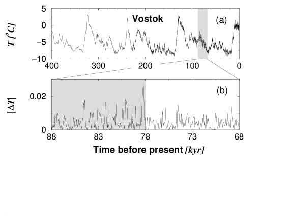
FIG. 1.: (a) Isotopic temperature record from the Vostok ice core [1]; the temperature $T$ is calculated from the hydrogen isotope ratio. (b) A typical example of the magnitude of temperature changes $|\Delta T_{i}|$. The magnitude series is clustered — big magnitudes are likely to be followed by big magnitudes suggesting the presence of correlations in the $|\Delta T_{i}|$ series.

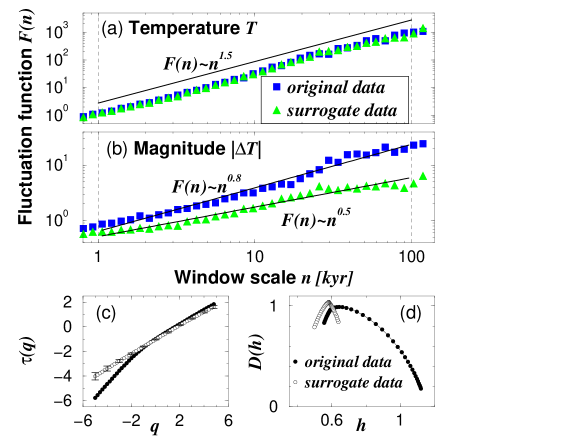
FIG. 2.: (a) The root mean square fluctuation $F(n)$ as a function of window scale $n$ in kyr for the Vostok temperature proxy data indicates strong correlations ( ). Before applying the second order DFA we sampled the data at 0.1kyr intervals [13]. The surrogate series (gray triangles) exhibits almost identical scaling confirming that correlations in the $T$ series are a linear measure. (b) $F(n)$ for the magnitude series, $|\Delta T|$, indicates strong correlations ( ) [17]. The magnitude series of the surrogate data (gray triangles) is uncorrelated (with exponent 0.5) demonstrating the nonlinearity of the data. (c) The multifractal analysis uses the wavelet transform modulus maxima method [19], with the 8-tap Daubechies discrete wavelet transform [20]. The exponents $\tau(q)$ are estimated by scaling function $Z_{q}(n)\sim n^{\tau(q)}$ [16] (0.8kyr $\leq n\leq$25.6kyr). The curvature in $\tau(q)$ reflects the multifractality of the temperature series ($\bullet$). The $\tau(q)$ of the surrogate series ($\circ$) is linear (10 realizations; the average $\pm$ 1 standard deviation is shown). (d) The multifractal spectrum, $D(h)\equiv hq-\tau(q)$ ($h\equiv d\tau/dq$), is much broader for the original data ($\bullet$) compared to the average $D(h)$ of the surrogate data ($\circ$) confirming that the underlying dynamics is nonlinear.

TABLE I.: Scaling results of the cores under consideration (0.1kyr sampling [13]). The DFA exponents for the original ($\alpha_{T}$) and magnitude ($\alpha_{|\Delta T|}$) series are obtained for window scales between 1kyr and $\sim$ 1/4 of the series length. The multifractal analysis is not accurate for short series, GISP, GRIP, Taylor Dome, and is not presented; nonetheless, the multifractal spectrum for these cores is broad as for Vostok (Fig. 2).

measure	GISP	GRIP	Taylor	Vostok
age	110kyr	225kyr	103kyr	422kyr
$\alpha_{T}$	1.14	1.18	1.4	1.54
$\alpha_{|\Delta T|}$	0.77	0.82	0.8	0.78

FIG. 3.: (a) An illustration of our model. Random switching between states $\eta_{i}$ determines the current $\eta_{i(t)}$ that interact with $\zeta(t)$ to change ice volume. The ice-sheet grows ($b=1$) until it crosses a critical ice volume $\xi$, where it breaks up ($b=-3$). Once the ice-sheet is totally melted ($V=0.01\xi$) growth starts again. (b) An example of a time series generated by our model; note that the y-axis is inverted to allow easier comparison with Fig. 1. The dashed lines indicate the maximal ($\xi$) and minimal ($0.01\xi$) ice-volume.

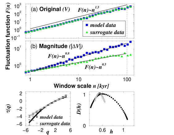
FIG. 4.: (a) As for the Vostok record (Fig. 2a), $F(n)$ indicates random walk behavior ( ). $F(n)$ remains unchanged after the surrogate data test (gray triangles). (b) $F(n)$ for the magnitude series reproduces the correlations observed for natural data (Fig. 2b). After the surrogate data test the magnitude series becomes uncorrelated indicating nonlinearity of our model. (c) The exponents $\tau(q)$ versus the moment $q$ for series generated by the model (10 realizations of 410kyr each, the average $\pm$ 1 standard deviation is shown) before ($\bullet$) and after ($\circ$) the surrogate data test. The exponents measured for window scales between 0.8kyr and 25.6kyr. The nonlinear dependence of $\tau(q)$ on $q$ is similar to the natural data (Fig. 2c) and becomes linear after the surrogate data test. (d) The multifractal spectrum $D(h)$ versus the exponent $h(q)$. As in the data (Fig. 2d) also here $D(h)$ is broad before applying the surrogate data test and becomes narrower afterward.

REFERENCES

- [1] J.R. Petit et al., Nature 399, 429 (1999).
- [2] J. Imbrie et al., Paleoceanography 7, 701 (1992); ibid. 8, 699 (1993).
- [3] B. Saltzman, Clim. Dyn. 5, 67 (1990).
- [4] H. Gildor H and E. Tziperman, Paleoceanography 15, 605 (2000); ibid. J. Geophys. Res.-Oceans 106, 9117 (2001).
- [5] E. Tziperman and H. Gildor, preprint.
- [6] M.A. Kominz and N.G. Pisias, Science 204, 171 (1979).
- [7] J.D. Pelletier, J. Climate 10, 1331 (1997).
- [8] C. Wunsch, preprint.
- [9] Data used here was downloaded from www.ngdc.noaa.gov/paleo/datalist.html.
- [10] J. Jouzel et al., Nature 329, 403 (1987).
- [11] M.F. Shlesinger, Ann. N.Y. Acad. Sci. 504, 214 (1987).
- [12] C.-K. Peng et al., Phys. Rev. E 49, 1685 (1994); A. Bunde et al., Phys. Rev. Lett. 85, 3736 (2000).
- [13] Before applying the scaling technique we evenly sampled the ice core data (50yr and 100yr). We find very similar DFA exponents for the different sampling rates. The scaling regime starts at 1kyr and is larger than the maximal spacing between consecutive values.
- [14] W. Dansgaard et al., Nature 364, 218 (1993).
- [15] T. Schreiber and A. Schmitz, Physica D 142, 346 (2000).
- [16] A series obeys scaling laws if . When the exponents are nonlinearly (or linearly) dependent on the series is multifractal (or monofractal). A multifractal (or monofractal) series has a nonlinear (or linear) underlying process. We use an advanced method of multifractality that accurately estimates the exponents of negative moments [19].
- [17] Y. Ashkenazy et al., Phys. Rev. Lett. 86, 1900 (2001); Y. Ashkenazy et al., preprint (cond-mat/0111396).
- [18] W.S. Broecker, Earth-Science Rev. 51, 137 (2000).
- [19] J.F. Muzy, E. Bacry, and A. Arneodo, Int. J. Bifurcat. Chaos 4, 245 (1994); E. Bacry, J. Delour, and J.F. Muzy, Phys. Rev. E 64, 026103 (2001).
- [20] I. Daubechies, Ten Lectures on Wavelets (SIAM, Philadelphia, PA, 1992).