Dynamical Mean Field Theory of Quantum Stripe Glasses

Abstract

We present a many body approach for non-equilibrium behavior and self-generated glassiness in strongly correlated quantum systems. It combines the dynamical mean field theory of equilibrium systems with the replica theory for classical glasses without quenched disorder. We apply this approach to study a quantized version of the Brazovskii model and find a self-generated quantum glass that remains in a quantum mechanically mixed state as $T\rightarrow 0$. This quantum glass is formed by a large number of competing states spread over an energy region which is determined within our theory.

I Introduction

The formation of glasses upon cooling is a well known phenomenon for classical liquids. Even without quenched disorder, the relaxation times become so large that a frozen non-ergodic state is reached before the nucleation into the crystalline solid sets in. The nucleation is especially easy to avoid if the material has many polymorphisms as does for example SiO₂. The system becomes unable to reach an equilibrium configuration on the laboratory time scale and exhibits aging and memory effects. While extrinsic disorder is widely acknowledged to lead to glassy phenomena in quantum systems, can a similar self generated glassiness occur for quantum liquids? Candidate materials for this behavior are strongly correlated electron systems which often exhibit a competition between numerous locally ordered states with comparable energies. Examples for such behavior are colossal magneto-resistance materials,mang01 ; Millis96 ; manganites cuprate superconductorsnmr01 ; nmr02 ; nmr03 ; nmr3b ; nmr04 ; msr01 ; msr02 ; msr03 and likely low density electron systemsAKS01 possibly close to Wigner crystallization.

The possibility of self generated quantum glassiness in such systems and the nature of the slow quantum dynamics has been little explored. Within a purely classical theory a “stripe glass” state was recently proposed in Refs.SW00 ; SWW00 . This proposal was stimulated by nuclear magnetic resonancenmr01 ; nmr02 ; nmr03 ; nmr3b ; nmr04 and $\mu$-spin relaxation experimentsmsr01 ; msr02 ; msr03 who found static or quasi-static charge and spin configurations similar to glassy or disordered systems. A prominent effect which reflects this slowing down was the “wipe-out” effect where below a certain temperature the typical time scales become so long that the resulting rapid spin lattice relaxation cannot be observed anymorenmr02 ; nmr03 ; nmr04 . More recently, the dynamical behavior of the stripe glass of Refs.SW00 ; SWW00 , as determined by Grousson et al.Grousson was found to be in quantitative agreement with NMR-experimentsnmr05 . Finally, recent $\mu$-spin experimentsmsr02 ; msr03 analyzed the freezing temperatures as function of charge carrier concentration and disorder concentration and found a quantum glass transition which was insensitive to the amount of disorder added to the system. This latter experiment, which seems to support a generic explanation for glassiness,not caused by impurities, also demonstrated the need for a more detailed investigation of the quantum regime of glassy systems. It is then important to develop appropriate theoretical tools to predict whether a given theoretical model for a quantum many body system will exhibit self-generated glassiness where the system forms a glass for arbitrary weak disorder.

In this paper we develop a general approach to self generated quantum glasses that combines the dynamical mean field theory (DMFT) of quantum many body systemsdmftreview1 ; dmftreview2 ; dmftreview3 with the replica technique of Refs.Mon95, ; MP991, which describes classical glasses without quenched disorder. In addition, we also go beyond strict mean field theory and estimate the spectrum of competing quantum states after very long times. This approach is applied to study a model with competing interactions which has a fluctuation induced first-order transition to a striped (2D) / lamellar (3D) phase. A quantum glass is shown to be in a quantum mechanical mixed state even at $T=0$, formed by a large number of states which can be considerably above the true ground state. Using the concept of an effective temperatureTool46 ; N98 ; CK93 for the distribution of competing ground states, our theory allows the investigation of glassy non-equilibrium dynamics in quantum systems using standard techniques of equilibrium quantum many body theory. On the mean field level, our theory is in complete agreement with the explicit dynamical non-equilibrium approach developed by Cugliandolo and LozanoCL99 for quenched disordered spin glasses with entropy crisis, which includes weak long-term memory effects and the subtle interplay of aging and stationary dynamics.

We find that when quantum fluctuations are weak, i.e., for a small quantum parameter, $c$ (for a definition see Eq.II below) , the glass transition resembles that of classical modelsKTW89 that exhibit a dynamical transition at a temperature $T_{\text{A}}$ (where mean field theory becomes non-ergodic) and a Kauzmann entropy crisis at $T_{\text{K}}<T_{\text{A}}$ if equilibrium were to be achieved. The actual laboratory glass transition is located between these two temperatures and depends for example on the cooling rate of the system. Beyond a critical $c$, $T_{\text{K}}$ and $T_{\text{A}}$ merge and the transitions change character. Within mean field theory, a discontinuous change of the relevant quantum mechanical states occurs at the glass transition. Even going beyond mean field, the system remains in a mixed quantum state however with a non-extensive number of relevant quantum states. Still, at the quantum glass transition a discontinuous change of the density matrix to a usual quantum liquid occurs. Put another way, a glass in contact with a bath at $T=0$ is essentially a classical object, qualitatively distinct from a quantum fluid, enforcing the quantum glass transition to be discontinuous. Our results clearly support the later scenario as can be seen in Fig.2 below.

In classical glass forming liquids an excess or configurational entropy with respect to the solid state due to an exponentially large number of metastable configurations emerges below $T_{\text{A}}$. Obviously, in the quantum limit a glass transition must be qualitatively different. Even a very large number of long lived excited states cannot compensate their vanishing Boltzmann weight at equilibrium for $T=0$. An exponentially large ground state degeneracy on the other hand is typically lifted by hybridization, saving kinetic energy. In Ref.KFI99, it was then argued that for a glassy quantum system the Edwards-Anderson order parameter vanishes continuously at the quantum glass transition (in contrast to the classical behavior). On the other hand, in Ref.Cugl, it was concluded that in certain spin glasses with quenched disorder the glass transition at sufficiently small $T$ is of first order.

The outline of this paper is as follows. In section II we introduce a quantized version of the Brazovskii model of micro-phase separation. We then discuss the replica approach used in this paper as well as the dynamical mean field theory employed for the solution of the problem in sections III and IV, respectively. Conclusions which are based on the approach developed here but which go beyond the strict mean field limit are discussed in section V. Finally we present a summary of our results in the concluding section VI. The equivalence of the “cloned-liquid” replica approach and the Schwinger-Keldysh theory of non-equilibrium quantum systems is presented in the appendix.

II The model

We consider a Bose system with field, $\varphi_{\mathbf{x}}$, governed by the action $\mathcal{S}\left[\varphi_{\mathbf{x}}\right]$ with competing interactions which cause a glass transition in the classical limit. Specifically we consider a system with action

$$\mathcal{S} = \frac{1}{2}\int d^{3}x\int d\tau\left(\left(\frac{\partial\varphi_{\mathbf{x}}}{\partial c\tau}\right)^{2}+r_{0}\varphi_{\mathbf{x}}^{2}+\frac{u}{2}\varphi_{\mathbf{x}}^{4}\right.$$

$$\left.+2q_{0}^{-2}\left(\left[\nabla^{2}+q_{0}^{2}\right]\varphi_{\mathbf{x}}\right)^{2}\right).$$

Here, $q_{0}$ is a wave number which supports strong fluctuations for momenta with amplitude $\left|\mathbf{q}\right|=q_{0}$, i.e. modulated field configurations. The classical version of the model, Eq.II, was shown by BrazovskiiBraz to give rise to a fluctuation induced first order transition to a lamellar or smectic state. Within equilibrium statistical mechanics, this ordered state gives the lowest known free energy. In Refs.SW00, ; SWW00, we demonstrated that, within non-equilibrium classical statistical mechanics, an alternative scenario is a self generated glass. Instead of the transition to a smectic state, metastable solutions built by a superposition of large amplitude waves of wavenumber $q_{0}$, but with random orientations and phases emergeWWJW . Those form the stripe glass state discussed in Ref. SW00, ; SWW00, . It is unclear so far whether the glassy solution occurs only if the ordered phase can be avoided by super-cooling or whether there is a parameter regime where the glass is favored regardless of the cooling rate.

In Eq.II we consider additional quantum fluctuations, characterized by the velocity, $c$. Clearly, quantum fluctuations reduce the tendency towards a fluctuation induced first order transition. This can be seen by evaluating the $\left\langle\varphi^{2}\left(x,\tau\right)\right\rangle$ within the spherical approximation. In the classical limit $\left\langle\varphi^{2}\left(x,\tau\right)\right\rangle\sim Tq_{0}^{2}r^{-1/2}$ with renormalized mass $r=r_{0}+u\left\langle\varphi^{2}\left(x,\tau\right)\right\rangle$ and the solution $r=0$ clearly does not exist. The same fluctuations which suppress the occurrence of a second order transition lead to a first order transition at the temperature where $r_{0}\simeq uTq_{0}^{2}r_{0}^{-1/2}$.Braz In the quantum limit the behavior is conceptually similar but fluctuations grow only logarithmically, $\left\langle\varphi^{2}\left(x,\tau\right)\right\rangle\sim q_{0}^{2}\log\left(\frac{\Lambda}{r}\right)$. For exponentially large correlation length $r^{-1/2}$ there should also be a  fluctuation induced first order transition to a smectic, which might be related to the state proposed in Ref.FKE, in the context of strongly correlated quantum systems. Another option however is the emergence of a stripe glass, even for large quantum fluctuations, which results in an amorphous modulated state instead. The investigation of this option will be the specific application of our theory. Before we go into specifics of the model, Eq.II, we develop a general framework for the description of self generated quantum glasses.

III The “cloned liquid” - replica approach

Competing interactions of a glassy system cause the ground state energy as well as the excitations to be very sensitive to small additional perturbations. In order to quantify this we introduce, following Ref.Mon95, , a static “ergodicity breaking” field $\psi$:

$$\mathcal{S}_{\psi}\left[\varphi\right]=\,\,\mathcal{S}\left[\varphi\right]+\frac{g}{2}\int d\tau d^{3}x\left(\psi_{\mathbf{x}}-\varphi_{\mathbf{x}}\left(\tau\right)\right)^{2}$$

and take the limit $g\rightarrow 0$ eventually. The coupling between $\varphi$ and $\psi$ will bias the original energy landscape in the “direction” of the configuration $\psi$, enabling us to count distinct configurations. Adopting a mean-field strategy, we assume that even in the quantum limit $\psi$ should be chosen as static variable, probing only time averaged configurations.

Introducing $\widetilde{f}_{\psi}=-T\log Z_{\psi}$, with the biased partition function $Z_{\psi}\,\,=\int D\varphi e^{-\mathcal{S}_{\psi}}$, $\widetilde{f}_{\psi}(T\rightarrow 0)$ corresponds to the ground state energy for a given $\psi$. If there are many competing ground states, it is natural to assume that $\widetilde{f}_{\psi}$ determines the probability, $p_{\psi}$, for a given configuration. If we identify the actual state of the system we gain the information $S_{c}=-\lim_{g\rightarrow 0}\int D\psi\,p_{\psi}\log p_{\psi}$. Maximizing this configurational entropy $S_{c}$ with respect to $p_{\psi}$ yields the usual result

$$p_{\psi}\propto\exp\left(-\widetilde{f}_{\psi}/T_{\text{eff}}\right),$$ (2)

where the effective temperature, $T_{\text{eff}}$ is the Lagrange multiplier enforcing the constraint that the typical energy is $\widetilde{F}=\lim_{g\rightarrow 0}\int D\psi\,p_{\psi}\widetilde{f}_{\psi}$. $T_{\text{eff}}$ is a measure for the width of the energy region within which the relevant ground state energies can be found. If the system is glassy, $T_{\text{eff}}>T$ and a quantum mechanically mixed state results even as $T\rightarrow 0$. Thus, a glass will not be in a pure quantum mechanical state (characterized by a single wave function) even at zero temperature.

Introducing the ratio $m=\frac{T}{T_{\text{eff}}}$ it follows $p_{\psi}\propto Z_{\psi}^{m}$, leading to

$$\widetilde{F} = \frac{\partial\left(mF\left(m\right)\right)}{\partial m}$$

$$S_{c} = \frac{m}{T_{\text{eff}}}\frac{\partial F\left(m\right)}{\partial m},$$

where we introduced $F=\widetilde{F}-T_{\text{eff}}S_{c}$ with

$$F\left(m\right)=-\lim_{g\rightarrow 0}\frac{T}{m}\log\int D\psi Z_{m}\left[\psi\right].$$

It is now possible to integrate out the auxiliary variable $\psi$, yielding an $m$-times replicated theory of the original variables $\varphi$ with infinitesimal inter-replica coupling:

$$\mathcal{S}=\sum_{\alpha=1}^{m}\mathcal{S}[\varphi^{\alpha}]-g\sum_{\alpha,\beta=1}^{m}\int d^{3}xd\tau d\tau^{\prime}\varphi_{\mathbf{x}}^{\alpha}\left(\tau\right)\varphi_{\mathbf{x}}^{\beta}\left(\tau^{\prime}\right),$$ (3)

similar to a random field model with infinitesimal randomness $g$. The major difference here is that in systems with a tendency towards self-generated glassiness, the initial infinitesimal randomness $g$ will self consistently be replaced by an effective, interaction induced, self-generated randomness. Specifically this will be the off diagonal element of the self energy in replica space.

At this point it is useful to discuss similarities and differences of the present approach if compared to the conventional replica approach of systems with quenched disorder. First, on a technical level, the replica index has to be analytically continued to $m=T/T_{\text{eff}}\leq 1$ and not to zero. This reflects the fact that slow metastable configurations do not equilibrate at the actual temperature, $T$, but at the effective temperature $T_{\text{eff}}$. In other words, the system has an essentially equal probability to evolve into states which are spread over a spectrum with width $T_{\text{eff}}$, even as $T\rightarrow 0$. If one applies the present approach to a system with explicit quenched disorder, where one can apply the conventional replica theory, and assumes replica symmetry, it turns out that $m$ corresponds to the break point of a solution with one step replica symmetry breaking of the conventional replica approach and both techniques give identical results. Alternatively one might also consider the model, Eq.II, in the limit of an infinitesimal random field with width $g$ and break point of a one step replica symmetry breaking $m$ solution. This implies that the present approach captures the essence of glassy behavior in systems with two very distinct typical time scales. This will become particularly clear if we compare our results with the one obtained within the solution of the dynamical Schwinger-Keldysh theory in the appendix. A more physical relationship between the two replica approaches can be obtained by realizing that the typical free energy of a frozen state, $\widetilde{F}$, can also be written in the usual replica language via

$$\widetilde{F}=\lim_{n\rightarrow 0}\frac{1}{n}\left(\overline{Z_{\psi}^{n}}-1\right)$$

where the average is performed with respect to the distribution function $p_{\psi}\propto Z_{\psi}^{m}$. The distribution function of the self generated randomness is non-Gaussian. For example if $m\rightarrow 1$, $e^{-\mathcal{S}_{\psi}\left[\varphi\right]}$ can also be interpreted as the generating functional of the distribution $p_{\psi}$.RMV01 It is because this distribution is characterized by “colored noise” that we find a self generated glassy state of the kind discussed here. Finally, if one replaces $\left(\left[\nabla^{2}+q_{0}^{2}\right]\varphi\right)^{2}$ in Eq.II by the usual $\left(\nabla\varphi\right)^{2}$-term (which is the $q_{0}\rightarrow 0$ limit after appropriate rescaling of $\varphi$, $c$, $u$. etc.) there is no glass as $g\rightarrow 0$, making evident that self-generated glassiness is ultimately caused by the uniform frustration of the finite $q_{0}$ problem where modulated configurations, $\varphi\left(\mathbf{x}\right)\varpropto\cos\left(\mathbf{q}_{0}\cdot\mathbf{x}\right)$, with $\left|\mathbf{q}_{0}\right|=q_{0}$ and arbitrary direction have low energy.

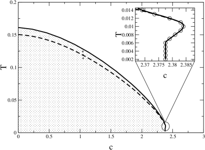
Figure 1: DMFT Phase diagram for the model Eq. 1 , within the one-loop self consistent screening approximation. The solid line represents $T_{\text{A}}$ whereas the dashed line represents $T_{\text{K}}$. The inset shows the low temperature region of the phase diagram where $T_{\text{A}}$ and $T_{\text{K }}$ have merged and the effective temperature at the transition is larger than $T$ ($m(T_{\textrm{A}})<1$). The line is simply a guide to the eye whereas the dots are the actual numerical result. The numerical simulations in the paper where carried out using the parameters $r_{0}=-6$, $q_{0}=0.3$ and $u=2\pi^{2}\left|r_{0}\right|$. The stars refer to the $(T,c)$ points of which the results in Fig.4 are shown.

IV Dynamical mean field theory

Due to the mean field character of the theory, it is appropriate to proceed by using the ideas of the DMFT for equilibrium many body systemsdmftreview1 ; dmftreview2 ; dmftreview3 and assuming that the self energy of our replicated field theory is momentum independent. Physically, ignoring the momentum dependence of the self energy might be justified by the fact that a glass transition usually occurs in a situation of intermediate correlations, i.e. when the correlation length of the liquid state is slightly larger but comparable to the typical microscopic length scales in the Hamiltonian.SWW00 The free energy of the system can be expressed in terms of the Matsubara Green’s function $G_{\mathbf{q}}^{\alpha\beta}\left(\omega_{n}\right)=\left\langle\varphi_{\mathbf{q}}^{a}(\omega_{n})\varphi_{-\mathbf{q}}^{b}(-\omega_{n})\right\rangle$ and the corresponding local (momentum independent) self energy $\Sigma^{\alpha\beta}\left(\omega_{n}\right)$ as

$$F\left(m\right)=\,\,\text{tr}\left(\Sigma G\right)-\text{tr}\log G+\Phi\left[G\right]\,\,,$$

where the self energy is given by $\Sigma=\frac{\delta\Phi\left[G\right]}{\delta G}$, and $\Phi\left[G\right]$ is diagrammatically well defined for a given systemKB61 .

The difference from the usual equilibrium DMFT approachdmftreview1 ; dmftreview2 ; dmftreview3 is the occurrence of off diagonal elements in replica space, allowing us to map the system onto a local problem with the same interaction but dynamical “Weiss” field matrix. This brings us to an effective zero dimensional theory similar to the mode-coupling theory of classical glasses.mc We furthermore make the ansatzMon95

$$G_{\mathbf{q}}^{\alpha\beta}\left(\omega_{n}\right)=\mathcal{G}_{\mathbf{q}}\left(\omega_{n}\right)\delta_{ab}+\mathcal{F}_{\mathbf{q}}\frac{\delta_{n,0}}{T},$$ (4)

with static off diagonal elements. A similar ansatz for the self energy leads to the following two Dyson equations for the diagonal and off diagonal propagators:

$$\mathcal{G}_{\mathbf{q}}\left(\omega_{n}\right) = \left[\mathcal{G}_{0,\mathbf{q}}^{-1}\left(\omega_{n}\right)-\Sigma_{\mathcal{G}}\left(\omega_{n}\right)\right]^{-1},$$

$$\mathcal{F}_{\mathbf{q}} = \Sigma_{\mathcal{F}}\mathcal{G}_{\mathbf{q}}\left(0\right)\left[\mathcal{G}_{\mathbf{q}}^{-1}\left(0\right)-m\Sigma_{\mathcal{F}}/T\right]^{-1}.$$ (5)

Glassiness is associated with finite values of the Edwards-Anderson order parameter, $\mathcal{F}_{\mathbf{q}}$, whereas for $\mathcal{F}_{\mathbf{q}}=0$ we recover the traditional theory of quantum liquids. The structure of the Dyson equation already gives us crucial informations on the nature of the glass transition. From Eq.5 follows immediately that, contrary to the classical case where glassiness can occur with $m=1$SW00 ; SWW00 , in the quantum limit ($T\rightarrow 0$) the only way $\mathcal{F}_{\mathbf{q}}$ can be non-zero is to have $m\rightarrow 0$ such that $m/T=1/T_{\text{eff}}\neq 0$. This imposes a constraint on the replica symmetry breaking structure in the quantum limit of the replica approach developed in Ref.Mon95, . Also, it is clear that $\Sigma_{\mathcal{F}}$ defines a new length scale of the problem that is associated with the glass transition.SWW00 In the classical glass transition the relation $m=1$ is satisfied at $T_{A}$. Then the two Dyson equations can be decoupled into an equilibrium, diagonal (in replica space) part, and a non-equilibrium, off-diagonal part. This allows us to interpret $\Sigma_{\mathcal{G}}$ as related with the equilibrium correlation length and to associate $\Sigma_{\mathcal{F}}$ with the Lindemann length, associated with the typical length scale of wandering of defects of the equilibrium structure, see Ref.SWW00 for details. However, it follows from the structure of the self-energies that, in the quantum limit, where $m<1$ at $T_{A}$, the two Dyson equations cannot be decoupled anymore. In this case, the two self-energies will combined define a correlation length and a Lindemann length which are not independent, but rather closely intertwined.

We solved the impurity problem within a self consistent large-$N$ approach, i.e. we generalize the scalar field $\varphi$ to an $N$-component vector and consider the limit of large-$N$ including first $1/N$-corrections. This approach was used earlier to investigate self generated glassiness in the classical limitSW00 ; SWW00 . In this limit it is also possible to solve the DMFT-problem exactlyWSKW02 , demonstrating that glassiness found in the approximate large-$N$ limit is very similar to the exact, finite $N$ theory and thereby supporting the applicability of the large $N$-expansion.

Within the self consistent large-$N$ approach, the diagonal and off diagonal element of the self energy are given as

$$\Sigma_{\mathcal{G}}\left(\omega_{n}\right) = \Sigma_{\mathcal{G}}^{H}-\frac{2}{N}\left(\mathcal{F}D_{\mathcal{G}}\left(\omega_{n}\right)+D_{\mathcal{F}}\mathcal{G}\left(\omega_{n}\right)\right)$$

$$+T\sum_{m}D_{\mathcal{G}}\left(\omega_{n}+\omega_{m}\right)\mathcal{G}\left(\omega_{m}\right)$$

$$\Sigma_{\mathcal{F}} = -\frac{2}{N}D_{\mathcal{F}}\mathcal{F},$$ (6)

with Hartree contribution

$$\Sigma_{\mathcal{G}}^{H}=-uT\sum_{m}\mathcal{G}\left(\omega_{m}\right)-u\mathcal{F}$$

as well as

$$D_{\mathcal{G}}\left(\omega_{n}\right) = \frac{1}{u^{-1}+\Pi_{\mathcal{G}}\left(\omega_{n}\right)+2\gamma\mathcal{FG}\left(\omega_{n}\right)}$$

$$D_{\mathcal{F}} = \frac{-\gamma\mathcal{F}^{2}D_{\mathcal{G}}^{2}\left(0\right)}{1+\gamma\mathcal{F}^{2}D_{\mathcal{G}}\left(0\right)/T_{\text{eff}}}$$ (7)

and bubble diagram $\Pi_{\mathcal{G}}\left(\omega_{n}\right)=\gamma T\sum_{m}\mathcal{G}\left(\omega_{n}+\omega_{m}\right)\mathcal{G}\left(\omega_{m}\right)$. Here $\mathcal{G}\left(\omega_{m}\right)=\int\frac{d^{3}q}{\left(2\pi\right)^{3}}\mathcal{G}_{\mathbf{q}}\left(\omega_{n}\right)$ and $\mathcal{F}=\int\frac{d^{3}q}{\left(2\pi\right)^{3}}\mathcal{F}_{\mathbf{q}}$ are the momentum averaged propagators. The DMFT is usually formulated on a lattice and it is possible to chose the same dimension (e.g. inverse energy) for the momentum dependent and momentum averaged propagator, by assuming the lattice spacing equal unity. In a continuum theory the role of the lattice spacing is played by the inverse upper cut off of the momentum integration $\Lambda$, which enters our theory in Eqs.7 through the constant $\gamma=\Lambda^{-3}$. In the case of the Hamiltonian, Eq.II, all momentum integrals are convergent as $\Lambda\rightarrow\infty$ and the scale which replaces the cut off is $q_{0}$, leading to $\gamma=q_{0}^{-3}$. We solved this set of self consistent equations numerically. Before we present the results we must discuss the stability of the ansatz, Eq.4.

The local stability of the replica symmetric ansatz, Eq.4 is determined by the lowest eigenvalue of the Hessian matrix $\frac{\delta^{2}F}{\delta G^{\alpha\beta}\delta G^{\gamma\delta}}$. Proceeding along the lines of Ref.dAT78, and diagonalization over the replica indices leads to the following matrix in momentum space

$$\mathcal{M}_{\mathbf{q},\mathbf{q}^{\prime}}=\delta\left(\mathbf{q}-\mathbf{q}^{\prime}\right)\mathcal{G}_{\mathbf{q}}^{-2}\left(0\right)+\mathcal{C}\,,$$ (8)

where

$$\mathcal{C}=\frac{\delta^{2}\Phi}{\delta G^{\alpha\beta}\delta G^{\alpha\beta}}-2\frac{\delta^{2}\Phi}{\delta G^{\alpha\beta}\delta G^{\alpha\delta}}+\frac{\delta^{2}\Phi}{\delta G^{\alpha\beta}\delta G^{\gamma\delta}},$$ (9)

with distinct $\alpha,\beta,\delta$ and $\delta$. Diagrammatically, $\mathcal{C}$ is a sum of diagrams with four external legs with at least two distinct replica indices. Thus, as $g\rightarrow 0$ the constant $\mathcal{C}$ vanishes if $\mathcal{F}_{\mathbf{q}}\rightarrow 0$, an observation which will be relevant in our discussion of the nature of the zero temperature glass transition as a function of $c$. We find for the lowest eigenvalue, $\lambda$, of $\mathcal{M}_{\mathbf{q},\mathbf{q}^{\prime}}$:

$$\mathcal{C}^{-1}=\int\frac{d^{3}q}{\left(2\pi\right)^{3}}\left(\mathcal{G}_{\mathbf{q}}^{-2}\left(0\right)+\lambda\right)^{-1}.$$ (10)

If $\lambda>0$ the mean-field solution is stable, whereas it is marginal for $\lambda=0$. The fairly simple result, Eq.10, for the stability of the replica structure is a consequence of the momentum independence of the self energy within DMFT which guarantees that $\Phi\left[G\right]$ only depends on the momentum averaged propagators. Otherwise $\mathcal{C}$ would depend on momentum, making the analysis of the eigenvalues of $\mathcal{M}_{\mathbf{q},\mathbf{q}^{\prime}}$ in Eq.8 much more complicated. Thus, the investigation of our problem within dynamical mean field theory is not only convenient to obtain solutions for $\mathcal{G}_{\mathbf{q}}\left(\omega_{n}\right)$ and $\mathcal{F}_{\mathbf{q}}$, it is also crucial to make progress in the analysis of the stability of this solution. We expect that it will be impossible to find a stable replica symmetric solution, Eq.4, once one goes beyond DMFT.

In real physical systems the slow degrees of freedom relax on a finite time scale $\tau_{\alpha}$ and the effective temperature $T_{\text{eff}}=T/m$ depends not only on the external parameters like $T$ and pressure, but also on the cooling rate, or equivalently on the time, $t_{w}$, elapsed after quenching and thus on the events which, for a finite range system, can take the system to different states of the spectrum characterized by $T_{\text{eff}}$. Accounting for these effects goes beyond a mean field treatment. However, for $t_{w}\ll\tau_{\alpha}$ mean field theory should apply. In fact, since within the mean field approach the time $\tau_{\alpha}$ is infinite, this is intrinsically the regime we are constrained to within the mean field treatment. Then, the most important configurations of the order parameter are those which allow the system to explore the maximum number of ergodic regions. The best way to achieve this, without being unstable, is through interconnecting saddle points.AC01 This leads to the marginal stability condition, $\lambda=0$, which we use to determine the effective temperature $T_{\text{eff}}^{0}$, which corresponds to the effective temperature right after a fast quench into the glassy state, i.e, $T_{\text{eff}}^{0}=T_{\text{eff}}(t_{w}\ll\tau_{\alpha})$:

$$\mathcal{C}\left(T_{\text{eff}}^{0}\right)^{-1}=\int\frac{d^{3}q}{\left(2\pi\right)^{3}}\mathcal{G}_{\mathbf{q}}^{2}\left(0,T_{\text{eff}}^{0}\right).$$ (11)

Within the large-$N$ approximation used to determine the propagator we can also evaluate the constant $\mathcal{C}$ of Eq.9, leading to

$$\mathcal{C}\left(T_{\text{eff}}^{0}\right)=\frac{2}{N}\left[2D_{\mathcal{G}}^{2}\left(0\right)\Pi_{\mathcal{F}}-\mathcal{D}_{\mathcal{F}}\right]$$ (12)

which is an implicit equation for $T_{\text{eff}}^{0}$. Note that, as we argued before, $\mathcal{C}$ vanishes for $\mathcal{F}\rightarrow 0$. Moreover, since the integral on the right hand side of Eq.11 is bounded from above, $\mathcal{C}$ and therefore $\mathcal{F}_{\mathbf{q}}$ must vanish discontinuously at the transition even for $T=0$. As explained above, from the structure of the Dyson equation in replica space it immediately follows that for $c$ larger than some value $c_{A}$, $T_{\text{eff}}^{0}/T$ must also jump discontinuously from $T_{\text{eff}}^{0}/T>1$ in the glass state to $T_{\text{eff}}^{0}/T=1$ in the quantum liquid state.

\psfrag{F}{$\mathcal{F}$}\includegraphics[width=216.81pt,keepaspectratio]{Fofc_bw.eps}

Figure 2: Low temperature behavior of the Edwards-Anderson order parameter as a function of the intensity of quantum fluctuations. The temperatures are in the region displayed in the inset of Fig. 1. Inset: dependence of the order parameter at the transition temperature $T_{\text{A}}$.

Together with Eq.11 we have a closed set of equations which describe the quantum glass within mean field theory. We have solved this set of equations for the model, Eq.II, and indeed found that there is a glassy state below a critical value for $c$. Most interestingly, for increasing $c$ (i.e.increasing quantum fluctuations) the rapidly quenched quantum glass, which at some point becomes unstable, undergoes a discontinuous reorganization of the density matrix upon entering the quantum liquid state. It is crucial to solve this many-body problem within some conserving approximation, i.e., based upon a given functional $\Phi\left(G\right)$, which must be simultaneously used to determine $\Sigma$ and $\mathcal{C}$. The set of equations was solved numerically. The Matsubara frequency convolutions were calculated on the imaginary time axis via Fast Fourier Transform algorithm using $2^{15}$ frequencies. This accuracy is needed mostly to be able to find solutions of Eqs.11 and 12 .

The transition line between the liquid and glassy states in the $(c,T)$ space is presented on Fig 1. Note that the low temperature (quantum regime) behavior is qualitatively different from the classical stripe glass. In the quantum limit, $T_{\text{A}}$ and $T_{\text{K}}$ merge and the effective temperature at the transition $T_{\text{eff }}^{0}\left(T_{\text{A}}\right)$ is always larger than $T_{\text{A}}$, i.e., $m<1$. Due to the reentrant character of the transition the quantum glass can also be reached by heating up the system. By generalizing Brazovskii’s theory of the fluctuation induced first order transition to the quantum case, we found a similar reentrance behavior for this equilibrium transition, suggesting that this peculiar shape of the phase border is determined by the increasing relevance of fluctuations with wave vector $\mathbf{q}=\left|q_{0}\right|$ as one crosses over from a quantum to a classical regime (see corresponding remarks made in sec.II). Another way the quantum glass can be reached is of course via a “$c$ quench”. Note also that the reentrant behavior we find within our approach happens at the point where numerically, at the same time, $T_{\text{A}}-T_{\text{K}}$ vanishes (to within numerical precision), $m\left(T_{\text{A}}\right)$ starts falling with a larger derivative (see the inset of Fig.3), and $\mathcal{F}\left(T_{\text{A}}\right)$ reaches a minimum (see inset of Fig. 2) before plateauing as $T\rightarrow 0$. This suggests that the reentrance behavior and the change of character of the transition are closely related. In Fig. 3 we show the dependence of the replica symmetry index $m=T/T_{\text{eff}}^{0}$ as function of $c$ for different temperatures.

In the classical limit, $c\rightarrow 0$, $\mathcal{F}_{\mathbf{q}}$ changes discontinuously at $T_{A}$, whereas $T_{\text{eff}}$ changes continuously $(m=1)$, i.e. the relevant metastable states - within which a classical glassy system gets trapped into - connect gradually to the relevant states which contribute to the liquid state partition function. A similar behavior in the quantum limit would imply that $T_{\text{eff}}$ and therefore $\mathcal{F}_{\mathbf{q}}$ and $\mathcal{C}$ vanish continuously at the quantum glass transition. However, as discussed above, this is not possible if one uses Eq.11 to determine the effective temperature. Thus, $T_{\text{eff}}$ changes discontinuously and one might expect a nucleation of liquid droplets within the unstable glass state to be important excitations which cause a quantum-melting of the glass. Even though one can formally introduce, along the lines of Ref.N98, , a latent heat $\delta Q=T_{\text{eff}}S_{c}$ at this transition, we do not know of a scenario which, within mean field theory, allows this energy to be realized within the laboratory. The appearance of a first order like transition as one enters the quantum regime, however without reentrance behavior, was first pointed out in Ref.Cugl, in a related case of spin glasses with quenched disorder.

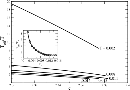
Figure 3: Dependence of the effective temperature as function of $c$ for different temperatures. Inset: dependence of $T_{\text{eff}}^{0}/T_{\text{A}}$ on $T_{\text{A}}$ in the low temperature regime displayed on the inset of Fig. 1.

Finally, we make contact between our theory and the Schwinger-Keldysh approach used in Ref.CL99, , which gives a set of coupled equations for the symmetrized correlation function $C_{\mathbf{x},\mathbf{x}^{\prime}}\left(\tau,t_{\text{w}}\right)=\frac{1}{2}\left\langle\left[\varphi_{\mathbf{x}}\left(t_{\text{w}}+\tau\right),\varphi_{\mathbf{x}^{\prime}}\left(t_{\text{w}}\right)\right]_{+}\right\rangle$ and the retarded response function $G_{\mathbf{x},\mathbf{x}^{\prime}}^{r}\left(\tau,t_{\text{w}}\right)=-i\theta\left(\tau\right)\left\langle\left[\varphi_{\mathbf{x}}\left(t_{\text{w}}+\tau\right),\varphi_{\mathbf{x}^{\prime}}\left(t_{\text{w}}\right)\right]_{-}\right\rangle$, where $\left[\,,\,\right]_{\pm}\equiv AB\pm BA$ . In the classical limit $C_{\mathbf{x},\mathbf{x}^{\prime}}\left(\tau,t_{\text{w}}\right)=\left\langle\varphi_{\mathbf{x}}\left(t_{\text{w}}+\tau\right)\varphi_{\mathbf{x}^{\prime}}\left(t_{\text{w}}\right)\right\rangle$as usual. If $t_{\text{w}}$, is comparable to $\tau$ the dynamics is complex and depends on the nature of the initial state (aging regime). On the other hand, for $t_{\text{w}}$ large compared to $\tau$, $C\left(\tau,t_{\text{w}}\right)$ and $G^{r}\left(\tau,t_{\text{w}}\right)$ are expected to dependent only on $\tau$ (stationary regime). Correspondingly, one can decompose the correlation function into aging and stationary contributions

$$C\left(\tau,t_{\text{w}}\right)=C_{\text{AG}}\left(\tau,t_{\text{w}}\right)+C_{\text{ST}}\left(\tau\right)\,,$$ (13)

and similarly for $G^{r}\left(\tau,t_{\text{w}}\right)$. Cugliandolo and KurchanCK93 showed within the mean field theory of classical spin glasses that one cannot decouple the stationary dynamics from the aging regime. Instead, the system establishes a “weak long term memory” and one has to solve for the entire time dependence. An elegant way to encode the aging dynamics is a generalized fluctuation dissipation theorem (FDT) $G_{\text{AG}}^{r}\left(\tau,t_{\text{w}}\right)=-T_{\text{eff}}^{-1}\frac{\partial}{\partial t_{\text{w}}}C_{\text{AG}}\left(\tau,t_{\text{w}}\right)$, with effective $T_{\text{eff}}$. This approach was generalized to the quantum case in Ref.CL99, .

As shown in the appendix, we find a complete equivalence of the Schwinger-Keldysh theory of Ref.CL99, , if applied to the quantized Brazovskii model, with our replica approach if we identify (after analytical continuation to real time): $\mathcal{G}\left(t\right)=G_{\text{ST}}^{r}\left(t\right)$and $\mathcal{F}=\lim_{t_{\text{w}}\rightarrow\infty}\lim_{t\rightarrow\infty}C_{\text{AG}}\left(t_{\text{w}},t\right)$. $T_{\text{eff}}^{0}$, which follows from marginality, Eq.11, is identical to the one of the generalized FDT, when we assume $t_{\text{w}}\ll\tau_{\alpha}$.BC01

V Aspects beyond the strict mean field theory

In this section we discuss several physically significant conclusions one can draw from our theory which go beyond the strict mean field limit. In particular we will discuss several aspects related to dynamical heterogeneity in glasses.

Going beyond mean field theory, for $t_{w}\gg\tau_{\alpha}$, the marginal stability cannot be sustained, since the system can save free-energy via droplet formation,KTW89 which drives the system towards equilibrium. As discussed in Ref.KTW89, , the free-energy gain is due to a gain in configurational entropy which is inhibited within mean field theory due to infinitely large barriers, but possible in finite subsystems where transitions between distinct metastable states becomes allowed. Thus, the glass might be considered as consisting of a mosaic pattern built of distinct mean field metastable states. The size of the various droplets forming the mosaic is determined by a balance of the entropic driving force (proportional to the volume of the drop) and the surface tensionKTW89 .

One way to account phenomenologically for such behavior within our theory is to assume that $T_{\text{eff}}$ becomes a time dependent quantityN98 and the exploration of phase space allows the system to “cool down” its frozen degrees of freedom by realizing configurational entropy. One would naturally expect $T_{\text{eff}}(t_{w})$ to decrease towards a value $T_{\text{eff}}^{\infty}$ until either $\lim_{N\rightarrow\infty}S_{c}(T_{\text{eff}}^{\infty})/N=0$ or $T_{\text{eff}}^{\infty}=T$. In the former case there is no extensive entropic driving force anymore which favors the exploration of phase space, whereas in the latter case the system has reached equilibrium but with, in general, finite remaining configurational entropy. These two regimes are separated by the Kauzmann temperature where $\lim_{N\rightarrow\infty}S_{c}(T_{\text{eff}}^{\infty})/N=0$ at $T_{\text{eff}}^{\infty}=T$ simultaneouslyKTW89 .We cannot, of course, calculate the explicit time dependence of $T_{\text{eff}}(t_{w})$ here. However, we can parametrically study $S_{c}(T_{\text{eff}})$ versus $T_{\text{eff}}$, i.e. keep the replica value $m$ an open parameter of the theory and analyze whether the trends for the variation of $S_{c}(T_{\text{eff}})$ at fixed temperature $T$ are sensible. Since we determined $m$ previously by the marginality condition, an effective temperature $T_{\text{eff}}<T_{\text{eff}}^{0}$ implies that the replicon eigenvalue is different from zero. We found numerically that $\lambda<0$, reflecting an instability of our solution likely related to some kind of dynamical heterogeneity. We argue that this heterogeneity is different for temperatures close to $T_{A}$ and $T_{K}$.

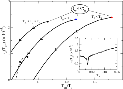
Figure 4: Parametric plot of the relaxation of $T_{\text{eff}}$ and $S_{c}$ for varying $t_{w}$ after quenches to the 3 points indicated by stars in the phase diagram Fig.1. In addition $S_{c}$ is shown for one point right at the quantum glass transition with $T_{A}=0.01>T$. The direction of evolution of the waiting time $t_{w}$ is indicated by the arrows. The system can relax from a state with marginal stability with $T_{\text{eff}}^{0}$ to 3 different final states as explained in the text. Inset: configurational entropy at the transition point as function of $T_{\text{A}}$.

We first discuss the behavior below but close to $T_{A}$ in the classical regime where marginality gives a continuous change of $m$, i.e. $T_{\text{eff}}^{\infty}\left(T_{A}\right)=T$. In this regime the system is close to equilibrium and it should be sensible to consider small fluctuations around the mean field solution. Such small fluctuations are then dominated by the eigenvectors of the replicon problem which correspond to the lowest eigenvalue. From Eq.8 we can easily determine the momentum dependence of this eigenvector, which can be interpreted as the fluctuating mean square of the long time correlation function $\mathcal{F}_{\mathbf{q}}$ away from its mean field value. It is given by

$$\Psi_{\mathbf{q}}=\Psi_{0}\frac{q_{0}^{4}}{\mathcal{G}_{\mathbf{q}}^{-2}-\lambda}$$ (14)

where, $\Psi_{0}$ is a normalization constant. At marginality, these modes in correlation function space are massless and thus easy to be excited. The typical length scale of these correlation function fluctuations are determined by $\mathcal{G}_{\mathbf{q=q}_{0}}^{-2}$, i.e. are confined to a length scale determined by $\Sigma_{\mathcal{G}}^{-1/2}$. Since this length is not the actual correlation length, but rather determined by the shorter Lindemann length discussed on Ref.SWW00, , the wandering of defects seem to set the scale on which the dynamics close to $T_{A}$ evolves. Thus correlations over the Lindemann length are fluctuating in space. Even though the fluctuating object is characterized by a rather short scale, its fluctuations are, of course, correlated over larger distances, as characterized by the nonlinear susceptibility $\chi^{\alpha\beta\gamma\delta}=\left\langle\varphi_{a}\left(x\right)\varphi_{\beta}\left(x\right)\varphi_{\gamma}\left(x\right)\varphi_{\delta}\left(x\right)\right\rangle$. $\chi^{\alpha\beta\gamma\delta}$ is the inverse of the Hessian and thus diverges if $\lambda\rightarrow 0$. Thus we conclude that close to $T_{A}$ this heterogeneity is driven by the correlation function fluctuations of shape $\Psi_{\mathbf{q}}$ of Eq.14. We believe that this “Goldstone” - type heterogeneity is very similar in character to the recent interesting approach to heterogeneity resulting from the assumption of a local time reparametrization invarianceCastillo02 . This is supported by the close relation between the reparametrization invariance and marginality as shown in Ref.CDD, . In addition, the approach of Ref.Castillo02, considers fluctuations relative to the mean field solution with stiffness proportional to the (mean field) Edwards-Anderson parameter. Thus, small fluctuations caused by the marginality of the mean field solution are considered, similar to the ones given in Eq.14 Further away from $T_{A}$ such a linearized theory is likely to break down because additional eigenvectors, not related to the marginal eigenvalue, become relevant and non-Gaussian fluctuations come into play. This should always be the case where $m$ is not close to unity, i.e. in the classical regime for temperatures below $T_{A}$ and everywhere in the quantum regime. One might expect droplet-physics to become important thenKTW89 .

In both cases it is useful to analyze the evolution of the spectrum of states of this formally unstable theory, particularly if the replica structure of the theory remains unchanged. As shown in Fig.1, we found numerically for the model, Eq.II, that for $t_{w}\gg\tau_{\alpha}$, three different possible final situations, result, depending on the relation between the bath temperature $T$ and the Kauzmann temperature $T_{K}$: (1) $T_{A}>T>T_{K}$, $T_{\text{eff}}$ will relax until it reaches $T$, but an excess entropy will remain. (2) $T=T_{K}$, $T_{\text{eff}}$ will relax until it reaches $T$, in a state with zero configurational entropy. (3) $T<T_{K}$, $T_{\text{eff}}$ will relax until all the excess entropy vanishes, but the system remains in a non-equilibrium state with $T_{\text{eff}}^{\infty}>T$. In this case there are still many (even though less than exponentially many) states, distributed according to a Boltzmann function with an effective temperature, $T_{\text{eff}}^{\infty}$. Their energies, $\tilde{f}_{\psi}$, differ by non-extensive amounts in a range of order $T_{\text{eff}}^{\infty}<T_{\text{eff}}^{0}$. At a critical value of the quantum parameter slightly below $c_{A}$ we find that $T_{A}$ and $T_{K}$ merge and the nature of the glass transition changes. The system is either in a quantum fluid or in a non-equilibrium frozen state and the identification of the glass transition using equilibrium techniques alone becomes impossible. Note however that in the quantum glass regime, even at temperatures $T$ arbitrarily close to $T_{\text{A}}$, for $t_{w}\gg\tau_{\alpha}$ we always obtain $\lim_{N\rightarrow\infty}S_{c}(T_{\text{eff}}^{\infty})/N=0$ for $T_{\text{eff}}^{\infty}>T$ (see dashed curve on Fig. 4).

VI Conclusion

In summary, we have presented an approach to self generated quantum glasses which enables the counting of competing ground state energies (quasi-classically of long lived metastable states) in interacting quantum systems. Technically very similar in form to the traditional quantum many body theory of equilibrium systems, it allows one to investigate whether a given system exhibits self generated glassiness as a consequence of the frustrating interactions. Slow degrees of freedom are assumed to behave classically and are shown to equilibrate to an effective temperature which is nonzero even as $T\rightarrow 0$ and which characterizes the width and rigidity of the energy landscape of the competing states of the system. Applied to the specific model, Eq.II, we do find a glass below a critical value for the quantum fluctuations. Using a marginality criterion to determine $T_{\text{eff}}$, we can generally show that quantum glass transitions are bound to be discontinuous transitions from pure to mixed quantum states. This leads to the interesting question of how quantum melting of the non-equilibrium quenched states can occur via nucleation of the corresponding quantum liquid state. Even going beyond mean field theory by assuming a time dependent effective temperature, we find that $T_{\text{eff}}$ saturates (at least for extremely long times) at a value $T_{\text{eff}}^{\infty}>T$. Finally we made connection to the dynamical approach for non-equilibrium quantum many body systems of Ref.CL99, , which shows that our theory properly takes into account the effects of aging and long term memory. We believe that the comparable simplicity of our approach allows it to apply our technique to a wide range of interesting problems in strongly interacting quantum systems.

This research was supported by an award from Research Corporation (J.S.), the Institute for Complex Adaptive Matter, the Ames Laboratory, operated for the U.S. Department of Energy by Iowa State University under Contract No. W-7405-Eng-82 (H.W.Jr. and J. S.), and the National Science Foundation grant CHE-9530680 (P. G. W.). H.W.Jr. acknowledges support from FAPESP project No. 02/01229-7

Appendix A Schwinger-Keldysh Formalism

In this section we apply the Schwinger and Keldysh close-time path Green function formalism applied to quantum glasses without quenched disorder. We follow closely Cugliandolo and LozanoCL99 , who applied the technique to spin glasses with quenched disorder. In this formalism response and correlation functions are treated as independent objects, coupled through a set of equations called Schwinger-Dyson equations. A perturbation theory scheme can be set up by considering the generalized matrix Green function

$$\widetilde{G}_{\mathbf{x},\mathbf{x}^{\prime}}\left(t,t^{\prime}\right)=\left(\begin{array}[]{cc}\,\,0&G_{\mathbf{x},\mathbf{x}^{\prime}}^{a}\left(t,t^{\prime}\right)\\ G_{\mathbf{x},\mathbf{x}^{\prime}}^{r}\left(t,t^{\prime}\right)&C_{\mathbf{x},\mathbf{x}^{\prime}}\left(t,t^{\prime}\right)\end{array}\right)$$ (15)

and self-energy

$$\widetilde{\Sigma}_{\mathbf{x},\mathbf{x}^{\prime}}\left(t,t^{\prime}\right)=\left(\begin{array}[]{cc}\,\,0&\Sigma_{\mathbf{x},\mathbf{x}^{\prime}}^{a}\left(t,t^{\prime}\right)\\ \Sigma_{\mathbf{x},\mathbf{x}^{\prime}}^{r}\left(t,t^{\prime}\right)&\Sigma_{\mathbf{x},\mathbf{x}^{\prime}}\left(t,t^{\prime}\right)\end{array}\right).$$

where

$$C_{\mathbf{x},\mathbf{x}^{\prime}}\left(t,t^{\prime}\right) = \frac{1}{2}\left\langle\left[\varphi_{\mathbf{x}}\left(t_{\text{w}}+\tau\right),\varphi_{\mathbf{x}^{\prime}}\left(t_{\text{w}}\right)\right]_{+}\right\rangle$$

$$G_{\mathbf{x},\mathbf{x}^{\prime}}^{r(a)}\left(t,t^{\prime}\right) = \mp i\theta\left(\pm\left(t-t^{\prime}\right)\right)\left\langle\left[\varphi_{\mathbf{x}}\left(t\right),\varphi_{\mathbf{x}^{\prime}}\left(t^{\prime}\right)\right]\right\rangle$$

In analogy to conventional perturbation theory, the components of $\widetilde{G}$ and $\widetilde{\Sigma}$ obey the Schwinger-Dyson equations

$$G_{\mathbf{q}}^{r} = G_{0\mathbf{q}}^{r}+G_{0\mathbf{q}}^{r}\otimes\Sigma_{\mathbf{q}}^{r}\otimes G_{\mathbf{q}}^{r}$$ (16)

$$C_{\mathbf{q}} = G_{\mathbf{q}}^{r}\otimes\left[G_{0\mathbf{q}}^{r-1}\otimes C_{0\mathbf{q}}\otimes G_{0\mathbf{q}}^{a-1}+\Sigma_{\mathbf{q}}\right]\otimes G_{\mathbf{q}}^{a}\,.$$ (17)

We use $\otimes$ to distinguish the matrix product over time (the time convolution) where $A\otimes B\,(t,t^{\prime})\equiv\int dsA(t,s)B\left(s,t^{\prime}\right)$ from the scalar (element-wise) product, where $A\,B\left(t,t^{\prime}\right)=A\left(t,t^{\prime}\right)B\left(t,t^{\prime}\right)$.

The first Schwinger-Dyson equation 16 is similar to conventional perturbation theory. However it is coupled to the second equation of $C\left(t_{1},t_{2}\right)$ which admits non-trivial solutions. For simplicity, we choose an initial condition such that $C_{0}=0$ and $\texttt{$\textrm{Im}$}G_{0}^{r}=0$. This leads to thermalization of $G^{r}$ (fulfillment of the FDT) in the absence of non-linearities, so it is an appropriate condition. Let us call $t_{2}=t_{w}$ and $t_{1}=t_{w}+\tau$, i.e., the correlations between instants separated by $\tau$ are measured after the waiting time $t_{w}$ has elapsed. The glassy dynamics appears in a regime of $t_{w}\rightarrow\infty$ and $\tau\rightarrow\infty$ . To proceed we assume that in this limit all correlation functions can be decomposed into a slow, non-time translation invariant, aging part ($AG$) and a fast, time translation invariant, stationary part ($ST$) like in Eq.13.

In this approach the stationary term decays on a characteristic time scale $\tau_{\beta}$ and it represents the correlations between degrees of freedom which are in equilibrium with the thermal reservoir at temperature $T$, i.e, retarded and Keldysh correlation functions are related by the FDT. The aging part on the other hand depends weakly on $t_{w}$ (aging phenomena) and varies slowly on $\tau$ in a characteristic large time scale $\tau_{\alpha}\gg\tau_{\beta}$, which allows us to neglect its $\tau$ derivatives. Moreover, as in reference CL99, , we enforce a relationship between $G_{\text{AG}}^{r}$ and $C_{\text{AG}}$ by defining an effective temperature $T_{\text{eff}}$ at which the long time correlations thermalize through a generalized FDT relation

$$G_{\text{AG}}^{r}\left(\tau,t\right)=-\frac{1}{T_{\text{eff}}\left(t\right)}\frac{\partial}{\partial t}C_{\text{AG}}\left(\tau,t\right)\,.$$ (18)

For $t\ll\tau_{\alpha}$ we can neglect the time dependence of $T_{\text{eff}}$, leading to a constant $T_{\text{eff}}\left(t\right)\rightarrow T_{\text{eff}}$.

Using the above assumptions, the first Schwinger-Dyson equation (16) in the stationary regime can be solved by a Fourier transform, which gives

$$\mathcal{G}_{\text{ST}\mathbf{q}}^{r}\left(\omega\right)=\frac{1}{\mathcal{G}_{0\mathbf{q}}^{r-1}\left(\omega\right)-\Sigma_{\text{ST}}^{r}\left(\omega\right)}\,.$$ (19)

Here we will explore solutions where $\,\,G_{\text{AG}}^{r}\left(\tau,t_{w}\right)$ is small but finite. This corresponds to the weak long term scenario where, even though $\lim_{\tau\rightarrow\infty}\lim_{t\rightarrow\infty}G_{\text{AG}}^{r}\left(\tau,t\right)\rightarrow 0$, the integral $\lim_{t\rightarrow\infty}\int_{0}^{t}dt^{\prime}G_{\text{AG}}^{r}\left(\tau,t^{\prime}\right)$ is still finite. In other words, we consider that the system keeps a vanishingly small memory of what happened in the past which, when accumulated over long times, gives a finite contribution to the dynamics. Thus, following along the lines of Ref.CL99, , we get for the for the aging regime

$$G_{\text{AG}\,\mathbf{q}}^{r}\left(\tau,t_{w}\right)=\Sigma_{\text{AG}}^{r}\left(\tau,t_{w}\right)\mathcal{G}_{\text{ST}\mathbf{\,q}}^{r}\left(0\right)^{2}\,.$$ (20)

Analogously, the second Schwinger-Dyson equation (17) can be solved for the same two regimes, yielding

$$G_{\text{ST}\mathbf{\,q}}^{K}\left(\omega\right)=\Sigma_{\text{ST}}^{K}\left(\omega\right)\mathcal{G}_{\text{ST}\mathbf{\,q}}^{r}\left(\omega\right)^{2}$$ (21)

and

$$C_{\text{AG}\,\mathbf{q}}\left(\tau,t_{w}\right)=\frac{\Sigma_{\text{AG}}\left(\tau,t_{w}\right)\mathcal{G}_{\text{ST}\mathbf{\,q}}^{r}}{\mathcal{G}_{\text{ST}\mathbf{\,q}}^{r}\left(0\right)^{-1}-\frac{1}{T_{\text{eff}}}\Sigma_{\text{AG}}^{K}\left(\tau,t_{w}\right)}\,.$$ (22)

Note that if we identify the real time correlation functions with the inter-replica correlation functions $\mathcal{F}$ and $\mathcal{G}$ as follows

$$\lim_{\tau\rightarrow\infty}\lim_{t_{w}\rightarrow\infty}C_{\text{AG}}\left(\tau,t_{w}\right) \equiv \mathcal{F}$$ (23)

$$\mathcal{G}_{\text{ST}}^{r}\left(\omega\right) \equiv \mathcal{G}\left(i\omega_{n}\rightarrow\omega+i\delta\right)$$ (24)

we get that the Schwinger-Dyson equations 19 and 22 are exactly equivalent to the replica equations in 5, provided that the self energies in the two schemes are also equivalent, i.e., $\Sigma_{\text{AG}}=-\Sigma_{\mathcal{F}}$ and $\Sigma_{\text{ST}}^{r}\left(\omega\right)=\Sigma_{\mathcal{G}}\left(i\omega_{n}\rightarrow\omega+i\delta\right)$. To prove this last requirement, we apply the same one-loop self-consistent screening perturbative scheme for the real time DMFT self energies $\widetilde{\Sigma}$. This gives

$$\widetilde{\Sigma}=\left(\begin{array}[]{cc}0&C\otimes D^{a}+D\otimes G^{a}\\ C\otimes D^{r}+D\otimes G^{r}&\,\,D^{a}\otimes G^{a}+D^{r}\otimes G^{r}+D\otimes C\end{array}\right)$$

where dressed interactions are given by

$$D^{r} = u+u\Pi^{r}\otimes D^{r}$$ (25)

$$D = u\Pi^{r}\otimes D+u\Pi\otimes D^{a}\,,$$ (26)

and the polarization bubbles are given by the element-wise products (no time or space convolutions)

$$\Pi^{r} = \gamma C\,G^{r}$$ (27)

$$\Pi = \gamma\left[\left(G^{a}\right)^{2}+\left(G^{r}\right)^{2}+C^{2}\right]\,.$$ (28)

The stationary and aging contributions to the self energies and polarizations can be calculated analogously by using the definitions (27) and (28) and separating the stationary from the aging contribution according to their asymptotic time behavior. This gives

$$\Sigma_{\text{ST}}^{r} = C_{\text{AG}}\otimes D_{\text{ST}}^{r}+D_{\text{AG}}\otimes G_{\text{ST}}^{r}$$

$$+C_{\text{ST}}\otimes D_{\text{ST}}^{r}+D_{\text{ST}}\otimes G_{\text{ST}}^{r}$$

$$\Sigma_{\text{AG}} = D_{\text{AG}}\otimes G_{\text{AG}}$$ (30)

and

$$\Pi_{\text{ST}}^{r} = \gamma\left(C_{\text{AG}}G_{\text{ST}}^{r}+C_{\text{ST}}G_{\text{ST}}^{r}\right)$$ (31)

and

$$\Pi_{\text{AG}} = \gamma C_{\text{AG}}^{2}$$ (32)

It is easy to verify accordingly that $\Pi_{\text{ST}}$ and $\Pi_{\text{ST}}^{r}$ are related by FDT at the temperature $T$ and $\Pi_{\text{AG}}$ and $\Pi_{\text{AG}}^{r}$ are related by the classical FDT at a temperature $T_{\text{eff}}$ . The last term in Eq.A is exactly the Matsubara convolution on (6). The remaining terms are calculated as follows:

$$\mathcal{D}_{\text{ST}}^{r}\left(\omega\right)=\frac{1}{u^{-1}+\Pi_{\text{ST}}^{r}\left(\omega\right)}$$ (33)

$$D_{\text{AG}}=\frac{-\Pi_{\text{AG}}\mathcal{D}_{\text{ST}}^{r}\left(\omega=0\right)}{\mathcal{D}_{\text{ST}}^{r}\left(\omega=0\right)^{-1}+\frac{1}{T_{\text{eff}}}\Pi_{\text{AG}}}$$ (34)

Using the relations 23 and 24 and performing the usual Matsubara sums we get,$\Pi_{\mathcal{F}}=\Pi_{\text{AG}}$ and $\Pi_{\mathcal{G}}\left(i\omega_{n}\rightarrow\omega+i0\right)=\Pi_{\text{ST}}^{r}\left(\omega\right)$ which yields $D_{\text{AG}}=D_{\mathcal{F}}$ and$D_{\mathcal{G}}\left(i\omega_{n}\rightarrow\omega+i0\right)=\mathcal{D}_{\text{ST}}^{r}\left(\omega\right)$. Therefore, equations (33), (34), (A), and (30) together prove that $\Sigma_{\text{AG}}=\Sigma_{\mathcal{F}}$ and $\Sigma_{\text{ST}}^{r}\left(\omega\right)=\Sigma_{\mathcal{G}}\left(i\omega_{n}\rightarrow\omega+i\delta\right)$and that there is a complete connection between replica and Schwinger-Keldysh formalisms. There is still one more independent equation, namely, Eq. 20, in the Schwinger-Keldysh formalism which bares no analog on the Dyson equations for the inter-replica correlation functions. However, if we integrate over $\mathbf{q}$ both sides of 20, substitute the definition $\Sigma_{\text{AG}}^{r}=C_{\text{AG}}\otimes D_{\text{AG}}^{r}+D_{\text{AG}}\otimes G_{\text{AG}}^{r}$ into 20 with $D_{\text{AG}}^{r}=\Pi_{\text{AG}}^{r}\mathcal{D}_{\text{ST}}^{2}\left(0\right)$we obtain

$$\left[2\mathcal{D}_{\text{ST}}^{2}\left(0\right)\Pi_{\text{AG}}^{K}-D_{\text{AG}}^{K}\right]\int\frac{d^{d}q}{\left(2\pi\right)^{d}}\mathcal{G_{\text{ST}}}_{\mathbf{q}}^{2}\left(0\right)=1$$ (35)

which, is exactly the marginality condition of the replica approach. This proves our previous statement that the saddle point condition gives the dynamical behavior at the time scales $t_{\mathrm{w}}\rightarrow\infty$, $\tau\rightarrow\infty$ with $t_{\mathrm{w}}\ll\tau_{\alpha}$. In this limit the effective temperature is not yet in equilibrium. In the opposite limit one cannot disregard the time dependence of $T_{\text{eff}}\left(t\right)$and it is thus not possible to write a closed form like equation (35). Nevertheless, the equilibrium approach based on the replica trick, together with the droplet relaxation picture enables us to access the behavior of $T_{\text{eff}}\left(t_{\text{w}}\right)$in the time limit $t_{\mathrm{\text{w}}}\gg\tau_{\alpha}$.

References

- (1) D. N. Argyriou, J. W. Lynn, R. Osborn, B. Campbell, J. F. Mitchell, U. Ruett, H. N. Bordallo, A. Wildes, C. D. Ling, Physical Review Letters 89, 036401 (2002).
- (2) A. J. Millis, Phys. Rev. B 53, 8434 (1996).
- (3) For a recent review on related aspects see: E. Dagotto, T. Hotta, and A. Moreo, Physics Reports 344, 1 (2001).
- (4) M.-H. Julien, F. Borsa, P. Carretta, M. Horvatic, C. Berthier, and C. T. Lin, Phys. Rev. Lett. 83, 604 (1999).
- (5) A. W. Hunt, P. M. Singer, K. R. Thurber, and T. Imai, Phys. Rev. Lett. 82, 4300 (1999).
- (6) N. J. Curro, P. C. Hammel, B. J. Suh, M. Hücker, B. Büchner, U. Ammerahl, and A. Revcolervschi, Phys. Rev. Lett. 85, 642 (2000).
- (7) J. Haase, R. Stern, C. T. Milling, C. P. Slichter, and D. G. Hinks, Physica C 341, 1727 (2000).
- (8) N. J. Curro, Journal of Physics and Chemistry of Solids 63, 2181(2002).
- (9) Ch. Niedermeyer, C. Bernhard, T. Blasius, A. Golnik, A. Moodenbaugh, and J. I. Budnik, Phys. Rev. Lett. 80, 3843 (1998).
- (10) C. Panagopoulos, J. L. Tallon, B. D. Rainford, T.Xiang, J. R. Cooper, and C. A. Scott, Phys. Rev. B 66, 064501 (2002).
- (11) J. L. Tallon, J. W. Loram, C. Panagopoulos, J. Low Temp. Phys. 131(3), 387 (2003)
- (12) E. Abrahams, S. V. Kravchenko, and M. P. Sarachik, Rev. Mod. Phys. 73, 251 (2001) and references therein.
- (13) J. Schmalian and P. G. Wolynes, Phys. Rev. Lett. 85, 836 (2000).
- (14) H. Westfahl Jr., J. Schmalian, and P. G. Wolynes, Phys. Rev. B 64, 174203 (2001).
- (15) M. Grousson, V. Krakoviack, G. Tarjus, and P. Viot, Phys. Rev. E 66, 026126 (2002)
- (16) B. Simovic, P. C.Hammel, M. Huecker, B. Buechner, and A. Revcolevschi, Phys. Rev. B 68, 012415 (2003)
- (17) D. Vollhardt, in Correlated Electron Systems, edited by V.J. Emery (World Scientific, Singapore, 1993).
- (18) A. Georges, G. Kotliar, W. Krauth, and M. J. Rozenberg, Rev. Mod. Phys. 68, 13-125 (1996).
- (19) T. Pruschke, M. Jarrell and J.K. Freericks, Adv. in Phys. 42, 187 (1995).
- (20) R. Monnason, Phys. Rev. Lett. 75, 2847 (1995).
- (21) M. Mezard and G. Parisi, Phys. Rev. Lett. 82, 747 (1999).
- (22) A. Q. Tool, J. Am. Ceram. Soc. 29, 240 (1946).
- (23) Th. M. Nieuwenhuizen, Phys. Rev. Lett. 80, 5580 (1998).
- (24) L. F. Cugliandolo, J. Kurchan, Phys. Rev. Lett. 71, 173 (1993).
- (25) L. F. Cugliandolo and G. Lozano, Phys. Rev. Lett. 80, 4979 (1998); Phys. Rev. B 59, 915 (1999).
- (26) T. R. Kirkpatrick and P. G. Wolynes, Phys. Rev. A 35, 3072 (1987); T. R. Kirkpatrick and D. Thirumalai, and P. G. Wolynes, Phys. Rev. A 40, 1045 (1989); T. R. Kirkpatrick and P. G. Wolynes, Phys. Rev. B 36, 8552 (1987);T. R. Kirkpatrick and D. Thirumalai, Phys. Rev. Lett. 58, 2091 (1987).
- (27) D. M. Kagan, M. Feigel’man and L. B. Ioffe, Zh. Eksp. Teor. Fiz. 116, 1450 (1999) [JETP 89, 781 (1999)].
- (28) L. F. Cugliandolo, D. R. Grempel, and C. A. da Silva Santos, Phys. Rev. Lett. 85, 2589 (2000).
- (29) S. A. Brazovskii, Zh. Exp. Teor. Fiz. 68, 175 (1975) [Sov. Phys. JEPT 41, 85 (2975)].
- (30) S. Wu, H. Westfahl Jr., J. Schmalian, and P. G. Wolynes, Chem. Phys. Lett. 359, 1 (2002).
- (31) S. A. Kivelson, E. Fradkin, V. J. Emery, Nature 393, 550-553 (1998).
- (32) V. G. Rostiashvili, G. Migliorini, and T. A. Vilgis, Phys. Rev. E 64, 051112 (2001).
- (33) G. Baym and L. P. Kadanoff, Phys. Rev 124, 287 (1961).
- (34) W. Götze, in Liquids, Freezing and Glass Transition, ed. J.-P. Hansen, D. Levesque and J. Zinn-Justin (North-Holland, Amsterdam, 1991), p. 287.
- (35) S. Wu, J. Schmalian, G. Kotliar, and P. G. Wolynes, cond-mat/0305404.
- (36) J. R. L. de Alameida and D. J. Thouless, J. Phys. A 11, 983 (1978).
- (37) Andrea Cavagna, Irene Giardina, Giorgio Parisi, J. Phys. A: Math. Gen. 34, 5317 (2001).
- (38) The relation between the dynamical theory and the TAP equations was discussed in G. Biroli and L. F. Cugliandolo, Phys. Rev B 64, 014206 (2001). Here, different TAP states are weighted with an effective temperature similar to our Eq.2.
- (39) H. E. Castillo, C. Chamon, L. F. Cugliandolo, M. P. Kennett, Phys. Rev. Lett. 88, 237201 (2002).
- (40) T. Temesvari, I. Kondor, C. De Dominicis, Eur.Phys.J.B 18, 493 (2000).