Large $N$ limit of the exactly solvable BCS model:
analytics versus numerics

Abstract

We have studied the numerical solutions of Richardson equations of the BCS model in the limit of large number of energy levels at half-filling, and compare them with the analytic results derived by Gaudin and Richardson, which in turn leads to the standard BCS solution. We focus on the location and density of the roots, the eigenvalues of the conserved quantities, and the scaling properties of the total energy for the equally spaced and the two-level models.

I) Introduction

One of the most studied models in Condensed Matter Physics is the BCS model of superconductivity, proposed by Bardeen, Cooper, and Schrieffer in 1957 BCS . The BCS model is usually formulated in the grand canonical ensemble, which is appropiated to systems with a macroscopic number of fermions. However for small systems, such as nuclei or ultrasmall metallic grains, one has to consider the canonical ensemble where the BCS wave function is not adequate.

Fortunately enough, there is a simplified version of the BCS model which is exactly solvable in the canonical ensemble. This occurs when the strengh of the pairing interaction between all the energy levels is the same. The exact solution of the reduced BCS model was obtained by Richardson in 1963 R1 ; R1bis ; RS , who also studied its consequences and properties in a series of papers in the 60’s and 70’s R-norm ; R-roots ; R-boson ; R-limit . The exactly solvable BCS model, in turn, is closely related to the rational spin model of Gaudin, defined in terms of a set of commuting Hamiltonians Gaudin ; G-book .

The integrability of the reduced BCS Hamiltonian was proved in 1997 by Cambiaggio, Rivas, and Saraceno (CRS) CRS , who constructed a set of conserved quantities in involution, commuting with the BCS Hamiltonian and closely related to the rational Gaudin’s Hamiltonians Gaudin . More recently Gaudin’s trigonometric model have been generalized, to include a $g$-term à la BCS, in references ALO ; DES . There are also bosonic pairing Hamiltonians satisfying the same type of equations as in the fermionic case R-boson ; DS ; DP . Generalizations of the $SU(2)$ BCS model to other Lie groups AFS and supergroups KM have been worked out. Both, the BCS and Gaudin’s models are intimately linked to conformal field theory B ; BF ; S , Chern-Simons theory AFS , and Integrable Models in Statistical Mechanics AFF ; ZLMG ; vDP (see ref. [Scomo, ] for a short review on these topics). The exact solution has also been used to study the effect of level statistics random and finite temperature Finite-T ; FFM on the ultrasmall metallic grains.

An important property of the exact solution is that the energy of the states and the occupation numbers agree, to leading order in the number of particles, with the BCS theory BCS . This result was obtained by Gaudin G-book and Richardson R-limit , using an electrostatic analogy of the Richardson’s equations, which have to be solved for finding the eigenstates of the BCS Hamiltonian. More recent applications of this electrostatic model to nuclear pairing can be found in ref. [DEP, ].

In the limit of large number of levels $N$, Richardson’s equations become integral equations, which can be solved with techniques of complex analysis G-book . This is sufficient to determine the location and density of roots, as well as the total energy of the ground state to leading order in $N$. To study higher order corrections of the ground state energy and the excitations, Richardson developed a multipole expansion of the fields appearing in the electrostatic analogue model R-limit . We shall follow Gaudin’s approach which is more geometrical, but use also some of the results obtained by Richardson.

The aim of this paper is to make a revision and precise comparison between the numerical solution and the analytic expressions for the location and density of roots of the Richardson’s equations, as proposed originally by Gaudin in his unpublished paper in 1968, which got finally published in his collected papers in 1995 G-book . The comparison will be made in the limit of large $N$ for the two-level model and the equally spaced model.

These models have been extensively used in Nuclear Physics since they were introduced by Hogaasen-Feldman Ho (two-level) and Richardson himself R-roots (equally spaced). The latter model has also been used to describe the physics of ultrasmall metallic grains grains ; Lanczos ; BvD ; DMRG ; Sch (for a review see ref. [vDR, ]). In the large $N$ limit the equally spaced model is superconducting for all values of atractive BCS couplings $g$, while the two-level model displays a quantum phase transition between a superconducting state and a normal state as a function of the BCS coupling constant.

The organization of the paper is as follows: in sections II and III we give a primer of the Richardson’s exact solution of the BCS model, together with its integrability. In section IV we introduce the electrostatic analogue model of BCS. In section V we review Gaudin’s continuum limit of the Richardson’s equations and their general solution, using complex analysis. In section VI we derive the gap and chemical potential BCS equations under the assumption that the roots of Richardson equations collapse into a single arc, and study in detail the two-level and equally spaced models. In section VII we present our numerical results and compare them with the analytic ones obtained in section VI. We also study the scaling properties of the roots and the ground state energy. In section VIII we present our conclusions and prospects. Finally, we describe in an appendix the conformal mappings associated to the equally spaced model.

II) Richardson’s exact solution of the reduced BCS model

The reduced BCS model is defined by the Hamiltonian BCS ; vDR ; grains

$$H_{BCS}=\frac{1}{2}\sum_{j,\sigma=\pm}\varepsilon_{j\sigma}c_{j\sigma}^{\dagger}c_{j\sigma}-G\sum_{j,j^{\prime}}c_{j+}^{\dagger}c_{j-}^{\dagger}c_{j^{\prime}-}c_{j^{\prime}+}\;,$$ (1)

where $c_{j,\pm}$ (resp. $c^{\dagger}_{j,\pm}$) is an electron annihilation (resp. creation) operator in the time-reversed states $|j,\pm\rangle$ with energies $\varepsilon_{j}/2$, and $G$ is the BCS dimensionful coupling constant. The sums in (1) run over a set of $N$ doubly degenerate energy levels $\varepsilon_{j}/2\;(j=1,\dots,N)$. We adopt Gaudin’s notation, according to which $\varepsilon_{j}$ denotes the energy of a pair occupying the level $j$ G-book . We shall assume that the energy levels are all distinct, i.e. $\varepsilon_{i}\neq\varepsilon_{j}$ for $i\neq j$. The Hamiltonian (1) is a simplified version of the reduced BCS Hamiltonian where all couplings have been set equal to a single one, namely $G$. Hereafter we shall refer to (1) simply as the BCS Hamiltonian.

Richardson had long ago solved this model exactly for an arbitrary set of levels, $\varepsilon_{j}$ R1 ; R1bis ; RS . To simplify matters, we shall assume that there are not singly occupied electronic levels. As can be seen from (1), these levels decouple from the rest of the system; they are said to be blocked, contributing only with their energy $\varepsilon_{j}/2$ to the total energy $E$. The above simplification implies that every energy level $j$ is either empty (i.e. $|{\rm vac}\rangle$), or occupied by a pair of electrons (i.e. $c^{\dagger}_{j,+}c^{\dagger}_{j,-}|{\rm vac}\rangle$). Denote the total number of electrons pairs by $M$. Then of course $M\leq N$. The most studied case in the literature corresponds to the half-filled situation, where the number of electrons, $N_{e}=2M$, equals the number of levels $N$ vDR . In the absence of interaction (i.e. $G=0$), all the pairs occupy the lowest energy levels, forming a Fermi sea. The pairing interaction promotes the pairs to higher energies and even for small values of $M$ or $G$ the levels are pair correlated Lanczos ; BvD ; DMRG ; vDR .

In order to describe Richardson’s solution one defines the hard-core boson operators

$$b_{j}=c_{j,-}c_{j,+},\qquad b_{j}^{\dagger}=c^{\dagger}_{j,+}c^{\dagger}_{j,-},\qquad N_{j}=b^{\dagger}_{j}b_{j}\;,$$ (2)

which satisfy the commutation relations,

$$[b_{j},b_{j^{\prime}}^{\dagger}]=\delta_{j,j^{\prime}}\;(1-2N_{j}).$$ (3)

The Hamiltonian (1) can then be written as

$$H_{BCS}=\sum_{j}\varepsilon_{j}b^{\dagger}_{j}b_{j}-G\,\sum_{j,j^{\prime}}\;b_{j}^{\dagger}b_{j^{\prime}}\;.$$ (4)

Richardson showed that the eigenstates of this Hamiltonian with $M$ pairs have the (unnormalized) product form R1 ; R1bis ; RS

$$|M\rangle=\prod_{\nu=1}^{M}B_{\nu}|{\rm vac}\rangle,\qquad B_{\nu}=\sum_{j=1}^{N}\frac{1}{\varepsilon_{j}-E_{\nu}}\;b^{\dagger}_{j}\;,$$ (5)

where the parameters $E_{\nu}$ ($\nu=1,\dots,M$) are, in general, complex solutions of the $M$ coupled algebraic equations

$$\frac{1}{G}=\sum_{j=1}^{N}\frac{1}{\varepsilon_{j}-E_{\nu}}-\sum_{\mu=1(\neq\nu)}^{M}\frac{2}{E_{\mu}-E_{\nu}}\;,\qquad\nu=1,\dots,M$$ (6)

which play the role of Bethe ansatz equations for this problem B ; BF ; S ; AFF ; ZLMG ; vDP ; Scomo . The energy of these states is given by the sum of the auxiliary parameters $E_{\nu}$, i.e.

$${E}(M)=\sum_{\nu=1}^{M}E_{\nu}.$$ (7)

The ground state of $H_{BCS}$ is given by the solution of eqs. (6) which gives the lowest value of ${E}(M)$. The (normalized) states (5) can also be written as R-norm

$$|M\rangle=\frac{C}{\sqrt{M!}}\sum_{j_{1},\cdots,j_{M}}\psi(j_{1},\dots,j_{M})b^{\dagger}_{j_{1}}\cdots b^{\dagger}_{j_{M}}|{\rm vac}\rangle,$$ (8)

where the sum excludes double occupancy of pair states and the wave function $\psi$ takes the form

$$\psi(j_{1},\cdots,j_{M})=\sum_{\cal P}\prod_{k=1}^{M}\frac{1}{\varepsilon_{j_{k}}-E_{{\cal P}k}}\;.$$ (9)

The sum in (9) runs over all the permutations, ${\cal P}$, of $1,\cdots,M$. The constant $C$ in (8) guarantees the normalization of the state R-norm (i.e. $\langle M|M\rangle=1$).

III) Integrability of the reduced BCS Hamiltonian

A well known fact about the BCS Hamiltonian is that it is equivalent to that of a XY spin model with long range couplings, and a “position dependent” magnetic field proportional to $\varepsilon_{j}$. To see this, let us represent the hard-core boson operators (2) in terms of the Pauli matrices as follows,

$$b_{j}=\sigma_{j}^{+},\qquad b_{j}^{\dagger}=\sigma_{j}^{-},\qquad N_{j}=\frac{1}{2}(1-\sigma^{z}_{j}),$$ (10)

in which case the Hamiltonian (4) becomes

$$H_{BCS} = H_{XY}+\frac{1}{2}\sum_{j}\varepsilon_{j}+G(N/2-M),$$ (11)

$$H_{XY} = -\sum_{j}\varepsilon_{j}t^{0}_{j}-\frac{G}{2}(T^{+}\;T^{-}+T^{-}\;T^{+}),$$

where the matrices

$$T^{a}=\sum_{j=1}^{N}t^{a}_{j},\qquad(a=0,+,-),\qquad\mbox{with}\qquad t^{0}_{j}=\frac{1}{2}\sigma^{z}_{j},\quad t^{+}_{j}=\sigma^{+}_{j},\quad t^{-}_{j}=\sigma^{-}_{j},$$ (12)

satisfy the $SU(2)$ algebra,

$$[T^{a},T^{b}]=f^{ab}_{c}T^{c},\qquad\mbox{with}\qquad f^{+0}_{+}=f^{0-}_{-}=-1,\quad f^{+-}_{0}=2,$$ (13)

whose Casimir is given by

$${\bf T}\cdot{\bf T}=T^{0}T^{0}+\frac{1}{2}(T^{+}T^{-}+T^{-}T^{+}).$$ (14)

This spin representation of the BCS model is the appropiate one to study its integrability, as it was shown by Cambiaggio, Rivas, and Saraceno (CRS), who constructed a set of operators, $R_{j}\;\;(j=1,\dots,N)$ CRS ,

$$R_{i}=-t^{0}_{i}-2g\;\sum_{j(\neq i)}^{N}\frac{{\bf t}_{i}\cdot{\bf t}_{j}}{\varepsilon_{i}-\varepsilon_{j}},\qquad(i=1,\dots,\Omega),$$ (15)

satisfying the properties

$$[H_{BCS},R_{i}]=[R_{i},R_{j}]=0,\qquad(i,j=1,\dots,N).$$ (16)

Let us denote by $\lambda_{j}$ the eigenvalue of $R_{j}$ acting on the state (8), i.e.,

$$R_{j}|M\rangle_{R}=\lambda_{j}|M\rangle_{R}.$$ (17)

CRS, unaware of Richardson’s solution, did not give an expression of $\lambda_{j}$ in their work. This was found in reference [S, ] using CFT techniques,

$$\lambda_{i}=-\frac{1}{2}+G\left(\sum_{\nu=1}^{M}\frac{1}{\varepsilon_{i}-E_{\nu}}-\frac{1}{2}\sum_{j=1(\neq i)}^{N}\frac{1}{\varepsilon_{i}-\varepsilon_{j}}\right),$$ (18)

which verifies $\sum_{i}\lambda_{i}=(M-N/2)$ upon using eqs. (6), so that it vanishes at half filling.

However CRS showed that $H_{XY}$ given in eq. (11) can be expressed in terms of the operators $R_{i}$ as

$$H_{XY}=\sum_{j}\varepsilon_{j}R_{j}+G\left(\sum_{j}R_{j}\right)^{2}-\frac{3}{4}GN.$$ (19)

Then using the eqs. (11), (18), and (6) one can show that ${E}(M)$ is indeed given by eq. (7). (For the two-level system the last term in (19) must be replaced by $-2G(N/4+1)N/4$ ).

IV) The Gaudin-Richardson’s electrostatic model of BCS

The equations (6) admit a 2 dimensional electrostatic analogy, which will be very useful in the study of the limit $N\rightarrow\infty$ G-book ; R-limit . Let us consider a set of $N$ charges $-1/2$ fixed at the positions $\varepsilon_{j}$ on the real axis, and a uniform field parallel to this axis with stregth $-1/2G$. The problem is to find the equilibrium positions of $M$ charges $+1$ at positions $E_{\mu}$ subject to their mutual repulsion, the attraction with the $-1/2$ charges, and the action of the uniform field. The 2D electrostatic potential is given by $W+W^{*}$, where $W$ reads,

$$W(\{E_{\mu}\},\{\varepsilon_{i}\}) = \frac{1}{2}\sum_{i,\mu}{\rm log}(\varepsilon_{i}-E_{\mu})-\sum_{\mu>\nu}{\rm log}(E_{\nu}-E_{\mu})$$ (20)

$$-\frac{1}{4}\sum_{i>j}{\rm log}(\varepsilon_{i}-\varepsilon_{j})+\frac{1}{2G}\left(\sum_{\mu}E_{\mu}-\frac{1}{2}\sum_{i}\varepsilon_{i}\right).$$

It is easy to see that the Richardson’s eqs. (6) arise as the stationary conditions $\partial W/\partial E_{\mu}=0$, while the conserved quantities (18) are proportional to the forces exerted on the fixed charges, i.e.

$$\lambda_{i}=2G\;\frac{\partial W}{\partial\varepsilon_{i}}.$$ (21)

The total energy (7) is the center of gravity of the charges $E_{\mu}$, which must be located symmetrically with respect to the real axis, i.e. if $E_{\mu}$ is a solution to the eqs. (6), then $E^{*}_{\mu}$ must also be a solution. This condition is fullfilled in two cases: i) either $E_{\mu}$ is real, or ii) $E_{\mu}$ and $E^{*}_{\mu}$ form a complex conjugate pair. The formation of these complex pairs is usually an indication of the superconducting properties of the ground state.

V) Continuum limit of Richardson’s equations

In reference [G-book, ] Gaudin proposed a continuum limit of the equations (6), in order to obtain the BCS formulas for the ground state energy and occupation number of levels. We shall follow closely this reference. This continuum limit is defined by taking the number of levels $N$ going to infinity, while keeping fixed the following quantities:

$$g=GN,\qquad M/N.$$ (22)

At the same time the pair energy levels $\varepsilon_{i}$ will be equivalent to a negative charge density $-\rho(\varepsilon)$ located on an interval $\Omega$ of the real axis. The total charge of this interval is given by

$$-\int_{\Omega}\rho(\varepsilon)d\varepsilon=-\frac{N}{2}\;.$$ (23)

We shall suppose that $\Omega$ is contained inside an interval $(-\omega,\omega)$. For example, in the BCS model with equally spaced levels, $\omega/2$ is equal to the Debye energy.

The basic asumption made by Gaudin, which is supported by numerical results, is that the solutions of eqs. (6) organize themselves into arcs $\Gamma_{k}\;(k=1,\dots,K)$, which are piece-wise differentiable and symmetric under reflection on the real axis. We shall call $\Gamma$ the union of all these arcs, and $r(\xi)$ the linear charge density of roots $E_{\mu}$ in the complex plane. Hence, the total number of pairs, $M$, and the total energy, $E$, are given by

$$\int_{\Gamma}r(\xi)\;|d\xi| = M,$$ (24)

$$\int_{\Gamma}\xi\;r(\xi)|d\xi| = E.$$ (25)

The continuum limit of eqs. (6) is

$$\int_{\Omega}\frac{\rho(\varepsilon)\;d\varepsilon}{\varepsilon-\xi}-P\int_{\Gamma}\frac{r(\xi^{\prime})\;|d\xi^{\prime}|}{\xi^{\prime}-\xi}-\frac{1}{2G}=0,\qquad\xi\in\Gamma,$$ (26)

which implies that the total electric field on every point of the arcs $\Gamma_{k}$ is null. On the other hand, the values of the conserved quantities (18) are given in the continuum by

$$\lambda(\varepsilon)=-\frac{1}{2}+G\left(\int_{\Gamma}\frac{r(\xi)\;|d\xi|}{\varepsilon-\xi}-P\int_{\Omega}\frac{\rho(\varepsilon^{\prime})\;d\varepsilon^{\prime}}{\varepsilon-\varepsilon^{\prime}}\right)\;,\qquad\varepsilon\in\Omega.$$ (27)

The formal solution of eqs. (26) can be found as follows. First of all, let us orient each arc $\Gamma_{k}$ from the point $a_{k}$ to the point $b_{k}$, and call $L_{k}$ an anticlockwise path encircling $\Gamma_{k}$. We look for an analytic field $h(\xi)$ outside $\Gamma$ and the set $\Omega$, such that

$$r(\xi)\;|d\xi|=\frac{1}{2\pi i}(h_{+}(\xi)-h_{-}(\xi))\;d\xi,\qquad\xi\in\Gamma,$$ (28)

where $h_{+}(\xi)$ and $h_{-}(\xi)$ denote the limit values of $h(\xi)$ to the right and left of $\Gamma$. This can be understood using the electrostatic equivalence, considering that the electric field presents a discontinuity proportional to the superficial density of charge when crossing such surface. Next, we define a function $R(\xi)$, with cuts along the curves $\Gamma_{k}$, by the equation

$$R(\xi)=\left[\prod_{k=1}^{K}(\xi-a_{k})(\xi-b_{k})\right]^{1/2},$$ (29)

and look for a solution which vanishes at the boundary points of $\Gamma$, in the form

$$h(\xi)=R(\xi)\;\int_{\Omega}\frac{\varphi(\varepsilon)\;d\varepsilon}{\varepsilon-\xi}\;.$$ (30)

This field has to be constant at infinity, hence the first $K-2$ moments of $\varphi$ must vanish, i.e.

$$\int_{\Omega}\;\varepsilon^{\ell}\;\varphi(\varepsilon)=0,\qquad 0\leq\ell<K-1.$$ (31)

This formula is empty if $K=1$. The contour integral surrounding the charge density $r(\xi)$ in (26) can be expressed as

$$\int_{\Gamma}\frac{r(\xi^{\prime})\;|d\xi^{\prime}|}{\xi-\xi^{\prime}}=\frac{1}{2\pi i}\int_{\Gamma}\frac{h_{+}(\xi^{\prime})-h_{-}(\xi^{\prime})}{\xi-\xi^{\prime}}\;d\xi^{\prime}=\frac{1}{2\pi i}\int_{L}\frac{h(\xi^{\prime})}{\xi-\xi^{\prime}}\;d\xi^{\prime},\qquad\xi\in{\bf C}\Gamma,$$ (32)

where ${\bf C}\Gamma$ is the region outside the curves in $\Gamma$. Using eqs. (29) and (30), one finds for the principal value of (32)

$$P\int_{\Gamma}\frac{r(\xi^{\prime})\;|d\xi^{\prime}|}{\xi-\xi^{\prime}}=\frac{1}{2\pi i}\int_{L}\frac{d\xi^{\prime}R(\xi^{\prime})}{\xi-\xi^{\prime}}\int_{\Omega}\frac{\varphi(\varepsilon)\;d\varepsilon}{\varepsilon-\xi^{\prime}}=-\int_{\Omega}\frac{\varphi(\varepsilon)R(\varepsilon)}{\varepsilon-\xi}d\varepsilon+\int_{\Omega}\varepsilon^{K-1}\varphi(\varepsilon)d\varepsilon,\qquad\xi\in\Gamma,$$ (33)

where we have deformed the contour of integration $L$ into two contours, one encircling the interval $\Omega$ (first term) and another one around the infinity (second term). We are assuming that $\Gamma$, and consequently $L$, do not cut the interval $\Omega$. The case where $L$ intersects $\Omega$ actually arises in the equally spaced model, and will be discussed later on.

Plugging eq. (33) into (26), we see that a solution is obtained provided the following equations are satisfied:

$$\varphi(\varepsilon)=\frac{\rho(\varepsilon)}{R(\varepsilon)},$$ (34)

$$\int_{\Omega}\varepsilon^{K-1}\frac{\rho(\varepsilon)}{R(\varepsilon)}d\varepsilon=\frac{1}{2G}\;,$$ (35)

which have to be suplemented by eq. (31), which can be rewritten as

$$\int_{\Omega}\varepsilon^{\ell}\frac{\rho(\varepsilon)}{R(\varepsilon)}d\varepsilon=0,\qquad 0\leq\ell<K-1.$$ (36)

The field $h(\xi)$ gives also the density of charges $r(\xi)$,

$$r(\xi)=\frac{1}{\pi}|h(\xi)|\;,\qquad\xi\in\Gamma,$$ (37)

and its value is given by replacing (34) into (30), i.e.

$$h(\xi)=R(\xi)\;\int_{\Omega}\frac{\rho(\varepsilon)}{R(\varepsilon)}\;\frac{d\varepsilon}{\varepsilon-\xi}\;,$$ (38)

whose value at infinity is $-1/2G$. Moreover, using eq.(32) and performing the same contour deformations that lead to eq.(33), one can show that the conserved quantities (27) are given by

$$\lambda(\varepsilon)=P\left[GR(\varepsilon)\;\int_{\Omega}\frac{\rho(\varepsilon^{\prime})}{R(\varepsilon^{\prime})}\;\frac{d\varepsilon^{\prime}}{\varepsilon^{\prime}-\varepsilon}\right]=\frac{G}{2}\left(h(\varepsilon+i\;0)+h(\varepsilon-i\;0)\right),\qquad\varepsilon\in\Omega,$$ (39)

so that $\lambda(\varepsilon)$ is the principal part of $h(\varepsilon)$ on the set $\Omega$. Finally the equations fixing the arcs $\Gamma_{k}$ are the equipotential curves of the total distribution, i.e.

$${\cal R}\int_{a_{k}}^{\xi}h(\xi^{\prime})\;d\xi^{\prime}=0,\qquad\xi\in\Gamma_{k}.$$ (40)

VI) The BCS equations

In this section we shall show how the BCS equations describing the ground state of the model can be derived from the formalism of section V G-book .

The basic assumption is that for the ground state all the roots $E_{\mu}$ form a single arc, i.e. $K=1$, leaving only two complex parameters $a\equiv a_{1}$ and $b\equiv b_{1}$, which shall be denoted as

$$a=\varepsilon_{0}-i\Delta,\qquad b=\varepsilon_{0}+i\Delta,$$ (41)

where $\varepsilon_{0}$ and $\Delta>0$ are real parameters.

From eq. (38) the electrostatic field is given by

$$h(\xi)=[(\xi-\varepsilon_{0})^{2}+\Delta^{2}]^{\frac{1}{2}}\int_{\Omega}\frac{\rho(\varepsilon)}{[(\varepsilon-\varepsilon_{0})^{2}+\Delta^{2}]^{\frac{1}{2}}}\frac{d\varepsilon}{\varepsilon-\xi}\;.$$ (42)

And the conserved quantities $\lambda(\varepsilon)$ can be derived from the eq. (39). Eq. (35) yields the BCS gap equation

$$\int_{\Omega}\frac{\rho(\varepsilon)\;d\varepsilon}{\sqrt{(\varepsilon-\varepsilon_{0})^{2}+\Delta^{2}}}=\frac{1}{2G}\;.$$ (43)

Similarly, eq. (24) becomes the chemical potential equation

$$M=\frac{1}{2\pi i}\int_{L}h(\xi)d\xi=\int_{\Omega}\left(1-\frac{\varepsilon-\varepsilon_{0}}{\sqrt{(\varepsilon-\varepsilon_{0})^{2}+\Delta^{2}}}\right)\rho(\varepsilon)d\varepsilon,$$ (44)

while eq. (25) gives the BCS expression for the ground state energy,

$$E=\frac{1}{2\pi i}\int_{L}\xi\;h(\xi)\;d\xi=-\frac{\Delta^{2}}{4G}+\int_{\Omega}\left(1-\frac{\varepsilon-\varepsilon_{0}}{\sqrt{(\varepsilon-\varepsilon_{0})^{2}+\Delta^{2}}}\right)\rho(\varepsilon)\;\varepsilon\;d\varepsilon.$$ (45)

Gaudin’s paper G-book contains a misprint in this equation since the term $-\frac{\Delta^{2}}{4G}$ is quoted as $-\frac{\Delta^{2}}{2G}$.

Comparing these equations with the corresponding ones in the BCS theory, we deduce the following relations between $\Delta$, $\varepsilon_{0}$, and $\rho(\varepsilon)$, and $\Delta_{BCS}$ (BCS gap), $\mu$ (chemical potential), and $n(\epsilon)$ (single particle energy density):

$$\Delta=2\Delta_{BCS},\qquad\varepsilon_{0}=2\mu,\qquad\rho(\varepsilon)=\frac{1}{4}\;n\left(\frac{\varepsilon}{2}\right).$$ (46)

The factor $1/4$, in the last term of (46), emerges from the normalization $1/2$ of the charge density $\rho(\varepsilon)$, times another factor $1/2$, due to the fact that the separation between energy pairs is twice the separation between single particle energy levels.

To determine the equation of the curve $\Gamma$ we define the complex variable

$$z=\sqrt{(\xi-\varepsilon_{0})^{2}+\Delta^{2}}=x+iy\;.$$ (47)

Using eqs. (40) and (42) we deduce for $\Gamma$,

$$0=\int_{\Omega}d\varepsilon\;\rho(\varepsilon)\left\{\frac{x}{\sqrt{(\varepsilon-\varepsilon_{0})^{2}+\Delta^{2}}}+\frac{1}{4}{\rm log}\frac{\left(x-\sqrt{(\varepsilon-\varepsilon_{0})^{2}+\Delta^{2}}\right)^{2}+y^{2}}{\left(x+\sqrt{(\varepsilon-\varepsilon_{0})^{2}+\Delta^{2}}\right)^{2}+y^{2}}\right\}.$$ (48)

Eqs. (43), (44), and (45) have been derived under the condition that $\Gamma$ does not cut the set $\Omega$, which requires that (48) has no solutions with $\xi\in\Omega$. In the equally spaced model the curve $\Gamma$ may intersect $\Omega$, so this case has to be treated with some care (see below).

Finally, the mean occupation of the energy level $\varepsilon_{j}$ can be computed from the formula $\langle N_{j}\rangle=\partial E/\partial\varepsilon_{j}$. In the large $N$ limit $\langle N_{j}\rangle$ can be shown to be given by G-book ; R-limit

$$N(\varepsilon)=\frac{1}{2}\left(1-\frac{\varepsilon-\varepsilon_{0}}{\sqrt{(\varepsilon-\varepsilon_{0})^{2}+\Delta^{2}}}\right),\qquad\varepsilon\in\Omega,$$ (49)

which agrees with the BCS result BCS . Next we shall apply the previous formalism to two models.

The two-level model

Let us suppose that we have two energy levels $\pm\varepsilon_{1}$, which can accomodate at most $N/2$ pairs each. The charge density is given by

$$\rho(\varepsilon)=\frac{N}{4}[\delta(\varepsilon+\varepsilon_{1})+\delta(\varepsilon-\varepsilon_{1})].$$ (50)

From eq. (44) we deduce that the chemical potential vanishes, i.e. $\varepsilon_{0}=0$, while the gap eq. (43) gives

$$\varepsilon_{1}^{2}+\Delta^{2}=g^{2},\qquad g=GN.$$ (51)

This equation implies that $g$ must be greater than $\varepsilon_{1}$. The total energy of this solution follows from (45),

$$E=-\frac{N}{4g}(\varepsilon_{1}^{2}+g^{2}).$$ (52)

Integrating eq. (42) we obtain the electric field, and accordingly the value of the conserved quantities

$$h(\xi)=\frac{N\xi}{2g}\frac{\sqrt{\xi^{2}+\Delta^{2}}}{\varepsilon_{1}^{2}-\xi^{2}}\quad\longrightarrow\quad\lambda(-\varepsilon_{1})=\frac{1}{8g\varepsilon_{1}}(2\varepsilon_{1}^{2}+g^{2}).$$ (53)

Similarly one finds $\lambda(\varepsilon_{1})=-\lambda(-\varepsilon_{1})$, in agreement with the condition $\sum_{i}\lambda_{i}=0$ derived in sect. III. The equation of the curve (48) becomes in this case

$$\frac{4x}{g}+{\rm log}\frac{(x-g)^{2}+y^{2}}{(x+g)^{2}+y^{2}}=0,$$ (54)

or equivalently

$$x^{2}+y^{2}+g^{2}=\frac{2xg}{{\rm th}(2x/g)}\;,$$ (55)

where $x$ and $y$ are given by eq. (47). In Gaudin’s paper G-book there is a misprint in eqs. (52) and (55).

From the numerical results shown in fig. 1, when $g>\varepsilon_{1}$ $\Gamma$ is an open arc between the imaginary points $\pm i\Delta$ in the complex $\xi$-plane. However when $g=\varepsilon_{1}$, in the limit when $N\rightarrow\infty$, the arc closes at the origin, and for $g<\varepsilon_{1}$ it remains closed surrounding the point $-\varepsilon_{1}$.

To treat this case Gaudin considers a general situation where $\Gamma$ is a closed curve surrounding a piece $\omega$ of $\Omega$ and defines a function $s(\xi)$ by the equation [G-book, ]

$$s(\xi)\;d\xi=r(\xi)\;|d\xi|.$$ (56)

Then eq. (26) is solved by

$$s(\xi)=\frac{i}{\pi}\left[\frac{1}{2G}+\int_{\omega}\frac{\rho(\varepsilon)\;d\varepsilon}{\varepsilon-\xi}-\int_{{\bf C}\omega}\frac{\rho(\varepsilon)\;d\varepsilon}{\varepsilon-\xi}\right],$$ (57)

which can be verified using $P\int_{\Gamma}d\xi^{\prime}/(\xi^{\prime}-\xi)=i\pi$, when $\xi\in\Gamma$. For the two-level model $s(\xi)$ is given by

$$s(\xi)=\frac{i}{\pi}\left[\frac{1}{2G}-\frac{N}{2}\frac{\varepsilon_{1}}{\varepsilon_{1}^{2}-\xi^{2}}\right],\qquad\xi\in\Gamma.$$ (58)

and eqs. (24) and (25) yield

$$M = \int_{\Gamma}d\xi\;s(\xi)=\int_{\omega}d\varepsilon\;2\rho(\varepsilon)=\frac{N}{2}\;,$$ (59)

$$E = \int_{\Gamma}d\xi\;\xi s(\xi)=\int_{\omega}d\varepsilon\;2\varepsilon\rho(\varepsilon)=-\frac{N}{2}\varepsilon_{1}\;,$$ (60)

Hence the state for $g<\varepsilon_{1}$ is a Fermi sea to leading order in $N$.

The conserved quantities are derived from an equation similar to (39), where $h(\xi)$ is replaced by $s(\xi)$, i.e.

$$\lambda(\varepsilon)=-i\frac{\pi G}{2}\left(s(\varepsilon+i0)+s(\varepsilon-i0)\right),\quad\varepsilon\in\omega\qquad\longrightarrow\qquad\lambda(-\varepsilon_{1})=\frac{1}{2}\left(1-\frac{g}{4\varepsilon_{1}}\right),$$ (61)

verifing, as in the previous case, the symmetry $\lambda(\varepsilon_{1})=-\lambda(-\varepsilon_{1})$.

To find the curve $\Gamma$ we integrate (58), and impose the result to be real accordingly to (56). Impossing the imaginary part of eq. (56) to vanish we obtain a diferential equation for the curve $\Gamma$, which is a check of consistency.

$${\cal R}\left(\frac{\xi-x_{0}}{g}+\frac{1}{2}\;{\rm log}\;\frac{\xi-\varepsilon_{1}}{\xi+\varepsilon_{1}}\right)=0,\qquad\xi\in\Gamma,$$ (62)

where $x_{0}$ is an integration constant, which has a non vanishing value, contrary to Gaudin’s assumption. Eq. (62) can be written as

$$x^{2}+y^{2}+\varepsilon_{1}^{2}=\frac{2x\varepsilon_{1}}{{\rm th}(2(x-x_{0})/g)},\qquad\xi=x+iy.$$ (63)

To find $x_{0}$ we have first to look for the point $\varepsilon_{0}$ where $\Gamma$ intersects the real axis. From fig. 1, the density of roots at this point vanishes, i.e. $s(\varepsilon_{0})=0$, which implies

$$\varepsilon_{0}=-\varepsilon_{1}\;\sqrt{1-g/\varepsilon_{1}}\;.$$ (64)

The value of $x_{0}$ is found by imposing that $\varepsilon_{0}$ belongs to the curve (63), namely

$$x_{0}=\varepsilon_{0}-\frac{g}{2}\;{\rm log}\frac{\varepsilon_{1}+\varepsilon_{0}}{\varepsilon_{1}-\varepsilon_{0}}\;.$$ (65)

As $g$ approaches $\varepsilon_{1}$ from below, both $\varepsilon_{0}$ and $x_{0}$ go to zero, and the curve (63) coincides with the curve (55) at the “critical point” $g=\varepsilon_{1}$.

Equally spaced model

Let us consider now a model with $N$ pair energy levels that are uniformly distributed in the interval $[-\omega,\omega]$, with a density $\rho(\varepsilon)=\rho_{0}$

$$\rho_{0}=\frac{N}{4\omega}\;.$$ (66)

The distance between the single particle energy levels, $d$, is given by $d=\omega/N=2\omega_{D}/N$, where $\omega_{D}$ is the Debye energy. This is the model used in most of the studies on ultrasmall superconducting grains vDR . At half-filling the number of pairs is $M=N/2$, which implies that $\varepsilon_{0}=0$ (see eq. (44)). On the other hand, the gap eq. (43) yields the standard result BCS

$$\Delta=\frac{\omega}{{\rm sinh}(1/g)},\qquad g=\frac{GN}{\omega}\;,$$ (67)

where $g$ is the usual dimensionless BCS coupling constant. Recall that $\Delta$ is twice the BCS gap $\Delta_{BCS}$. The total energy of the BCS ground state can be derived from (45),

$$E=-\frac{\omega^{2}}{4d}\;\sqrt{1+\left(\frac{\Delta}{\omega}\right)^{2}}\;,$$ (68)

while the energy of the Fermi sea state is given by

$$E_{FS}=-\frac{\omega^{2}}{4d}-\frac{GN}{2}\;.$$ (69)

The condensation energy is defined as $E_{C}=E-E_{FS}$, which in the weak coupling limit, where $\Delta\ll\omega$, behaves as

$$E_{C}\sim-\frac{\Delta_{BCS}^{2}}{2d}\;,$$ (70)

the well known result.

Next, we shall study the shape of the arcs in this model. The electrostatic field $h(\xi)$ is given by

$$h(\xi)=\rho_{0}\;\log{\frac{(\xi-\omega)(\Delta^{2}-\xi\omega+\sqrt{(\Delta^{2}+\xi^{2})(\Delta^{2}+\omega^{2})}}{(\xi+\omega)(\Delta^{2}+\xi\omega+\sqrt{(\Delta^{2}+\xi^{2})(\Delta^{2}+\omega^{2})}}}\;.$$ (71)

To simplify matters, Gaudin considered the limit $\Delta\ll\omega$, where eq. (71) becomes

$$h(\xi)=\rho_{0}\;\log{\frac{\xi-\sqrt{\Delta^{2}+\xi^{2}}}{\xi+\sqrt{\Delta^{2}+\xi^{2}}}},\qquad|\xi|\ll\omega.$$ (72)

The conserved quantities $\lambda(\varepsilon)$ are given by

$$\lambda(\varepsilon)=\frac{g}{4}\log{\frac{|(\varepsilon-\omega)(\Delta^{2}-\varepsilon\omega+\sqrt{(\Delta^{2}+\varepsilon^{2})(\Delta^{2}+\omega^{2})}|}{|(\varepsilon+\omega)(\Delta^{2}+\varepsilon\omega+\sqrt{(\Delta^{2}+\varepsilon^{2})(\Delta^{2}+\omega^{2})}|}}\quad\stackrel{{\scriptstyle|\varepsilon|\ll\omega}}{{\longrightarrow}}\quad\frac{g}{4}\log{\frac{|\varepsilon-\sqrt{\Delta^{2}+\varepsilon^{2}}|}{|\varepsilon+\sqrt{\Delta^{2}+\varepsilon^{2}}|}}\;.$$ (73)

In the low energy approximation the equation of the equipotential curves passing through the points $\varepsilon_{0}\pm i\Delta$ is given by

$${\cal R}\left[\xi\;{\rm log}\frac{\xi-\sqrt{\Delta^{2}+\xi^{2}}}{\xi+\sqrt{\Delta^{2}+\xi^{2}}}+2\sqrt{\Delta^{2}+\xi^{2}}\right]=0.$$ (74)

This curve cuts the real axis inside the interval $[-\omega,\omega]$, which contradicts the assumptions made so far. From numerical studies we can see that for weak couplings only a fraction of energies $E_{\mu}$ form complex conjugated pairs, which in the limit $N\rightarrow\infty$ organize themselves into arcs, while the other energies remain real and located between the lower energy levels (see the appendix for more details on this issue). Taking this into account and using contour arguments, it can be shown that the BCS eqs. (43), (44), and (45) also hold in cases where $\Gamma$ cuts the energy interval $\Omega$.

In the general case the curve $\Gamma$ is given by the equation

$${\cal R}\left[i\xi\;\arcsin{\sqrt{\frac{1+\xi^{2}/\Delta^{2}}{1-\xi^{2}/\omega^{2}}}}+\omega\;{\rm Argsinh}{\sqrt{\frac{\Delta^{2}+\xi^{2}}{\omega^{2}-\xi^{2}}}}\right]=0.$$ (75)

In the limit $\Delta\ll\omega$ eq. (75) turns into (74). We show in the appendix that for $\Delta>\omega$ the arc $\Gamma$ does not touch the interval $[-\omega,\omega]$ and all the roots $E_{\mu}$ are complex. This happens for $g>g_{0}=1.13459$ $(\sinh 1/g_{0}=1)$.

VII) Numerical results

In this section we present the comparison between the analytic results derived in section VI, and the numerical ones obtained by solving directly the Richardson’s eqs. (6) for the models considered above.

Two-level model

In this model there are two energy levels, $\pm\varepsilon_{1}$, with a degeneracy $N/2$. Hence the Richardson eqs. (6) become

$$\frac{1}{G}=\frac{N}{2}\left(\frac{1}{\varepsilon_{1}-E_{\nu}}-\frac{1}{\varepsilon_{1}+E_{\nu}}\right)-\sum_{\mu\neq\nu}^{M}\frac{2}{E_{\mu}-E_{\nu}}\;,$$ (76)

with $M=N/2$. The total number of solutions of this system of equations is given by the combinatorial number $C^{N}_{M}$. The solution which corresponds to the ground state of the BCS Hamiltonian is the one for which $E_{\mu}(G)\rightarrow-\varepsilon_{1},\;\forall\mu$ in the limit where $G\rightarrow 0$. For any non zero value of $G$, all the roots $E_{\mu}$ form complex conjugate pairs surrounding the lower energy $-\varepsilon_{1}$.

The reduced coupling constant for this case is taken as $g=GN$. Our numerical results are presented in units of $\varepsilon_{1}$, which is equivalent to set $\varepsilon_{1}=1$.

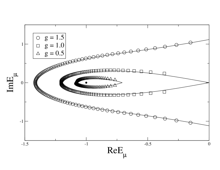
Figure 1: Plot in the $\xi$-plane of the solutions of eq. (76) for M=100 and three values of $g$. The continuous lines are the theoretical curves (55) (with the change of variables (47)) for $g=1.5,1$; and (63) for $g=0.5$. All the energies are in units of $\varepsilon_{1}$.

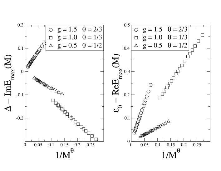
Figure 2: Plots of $\Delta-{\rm Im}\;E_{max}(M)$ and $\varepsilon_{0}-{\rm Re}\;E_{max}(M)$ versus $M^{-\theta}$, for the two-level model. $\varepsilon_{0}$ and $\Delta$ are given in eqs. (80) and (83), while numerical values of $\theta$ are given in table 1.

In fig. 1 we plot the distribution of the $M=100$ roots $E_{\mu}$, for three different values of the coupling constant $g=GN$, together with the analytic curves derived in section VI. There is an optimal agreement between the numerical and analytic results in the three regimes: normal ($g<\varepsilon_{1}$), critical ($g=\varepsilon_{1}$), and superconducting ($g>\varepsilon_{1}$). As we increase the value of $M$ up to 800 pairs, the fit of the numerical data to the analytical curves improves, and in the limit $M\rightarrow\infty$ the discrete roots collapse into the continuous curves. In particular, the complex roots $E_{max}(M)$ and $E_{max}^{*}(M)$, whose real part lies closer to $\varepsilon_{0}$, approach their continuum limit value, namely

$$\lim_{M\rightarrow\infty}E_{max}(M)=\varepsilon_{0}+i\Delta,$$ (77)

where

$$\varepsilon_{0} = \left\{\begin{array}[]{cll}0&&g\geq\varepsilon_{1}\\ -\varepsilon_{1}\;\sqrt{1-g/\varepsilon_{1}}&&g\leq\varepsilon_{1}\end{array}\right.,$$ (80)

$$\Delta = \left\{\begin{array}[]{cll}\sqrt{g^{2}-\varepsilon_{1}^{2}}&&g\geq\varepsilon_{1}\\ 0&&g\leq\varepsilon_{1}\end{array}\right.,$$ (83)

in agreement with eqs. (51) and (64).

Fig. 2 shows the following scaling behaviour $E_{max}(M)$:

$$E_{max}(M)-(\varepsilon_{0}+i\Delta)\sim\frac{1}{M^{\theta}}\;,$$ (84)

where the exponent $\theta$ depends on the regime of the system. The numerical and analytic results of $\theta$ are given in table 1:

$\theta$	$g=1.5\;\varepsilon_{1}$	$g=1.0\;\varepsilon_{1}$	$g=0.5\;\varepsilon_{1}$
analytical	2/3	1/3	1/2
numerical $(\Delta)$	0.635	0.329	0.446
numerical $(\varepsilon_{0}$)	0.672	0.328	0.513

Table 1.- Numerical and analytical values of the exponent $\theta$ appearing in eq. (84). The numerical values are extracted from the real and imaginary parts of $E_{max}(M)$.

The analytical value of $\theta$ can be derived as follows. For $M$ sufficiently large we can write

$$E_{max}(M)=(\varepsilon_{0}+i\Delta)+\delta\xi,$$ (85)

where $\delta\xi$ is a small number. Using eqs. (53), (56) and (58), the density of roots $r(E_{max})$ behaves as

$$r(E_{max})\sim AM(\delta\xi)^{\nu},\qquad\nu=\left\{\begin{array}[]{cc}1/2&g>\varepsilon_{1}\\ 2&g=\varepsilon_{1}\\ 1&g<\varepsilon_{1}\end{array}\right.,$$ (86)

where $A$ is a parameter which only depends on $g$ and $\varepsilon_{1}$. The magnitude of $\delta\xi$ can be fixed by imposing the existence of at least one root in the interval $(\varepsilon_{0}+i\Delta,\varepsilon_{0}+i\Delta+\delta\xi$), namely

$$1=r(E_{max})\;|\delta\xi|\sim AM\;|\delta\xi|^{\nu+1}\quad\longrightarrow\quad\delta\xi\sim\frac{1}{M^{\frac{1}{1+\nu}}}\;,$$ (87)

which is the desired result (84) with $\theta=1/(1+\nu)$.

Figure 3: Density of roots $r(E)/M$ as a function of the arc length. The continuous curves give the analytic result while the step like curves are the numerical results obtained for M= 800 and three values of $g$. The total length of the curve has been divided into 50 parts. The height of each part is the fraction of roots $E_{\mu}$ per unit length $\delta E$.

Figure 4: Plot of $e_{\infty}-e(M)$ versus $1/M$ for the two-level-model and different values of $g$. The continuous lines are given by eqs. (88) for $g\neq\varepsilon_{1}$, and eq. (89) for $g=\varepsilon_{1}$.

As we have seen in fig. 1, the roots $E_{\mu}$ lie on the analytic curves to a very good degree of approximation. A further check of the analytic solution is to compare the density of roots $r(\xi)$, which is given by $r(E)=|h(E)|/\pi$ for $g\geq\varepsilon_{1}$ (see eq. (37)), and by $r(\xi)=|s(\xi)|$ for $g\leq\varepsilon_{1}$ (see eq. (56)). In fig. 3 we plot the fraction of roots per unit length $r(E)/M$ as a function of the arc length $s\in[-1,1]$, where the $s=\pm 1$ corresponds to the end points of the arc $\Gamma$. The agreement is extremely accurate for $M=800$.

The value of the conserved quantities obtained in eq. (53) also agree with the numerical ones in the large $N$ limit, in the three different regimes.

Finally, it is interesting to study the behaviour of the energy as a funtion of the number of pairs $M$. The leading term is given by eq. (52) for $g\geq\varepsilon_{1}$ and by eq. (60) for $g\leq\varepsilon_{1}$. In fig. 4 we plot $e_{\infty}-e(M)$ versus $1/M$, where $e(M)=E(M)/M$ is the energy per pair. The linear behaviour of the numerical data means that the next leading correction to $E(M)$ is a constant term, $E_{1}$, whose value is given by the analytic expression

$$-E_{1}/M=e_{\infty}-e(M)=\left\{\begin{array}[]{lcl}(g-\frac{1}{2}\Delta)/M&&g\geq\varepsilon_{1}\\ (\varepsilon_{1}-|\varepsilon_{0}|)/M&&g\leq\varepsilon_{1}\end{array}\right.,$$ (88)

where $\Delta$ and $\varepsilon_{0}$ are given by eqs. (51) and (64) respectively. The formula for $g>\varepsilon_{1}$ has been derived by Richardson in ref. [R-limit, ], studying the next to leading order of the electrostatic model. The formula for $g<\varepsilon_{1}$ is an educated guess which needs a proof. At $g=\varepsilon_{1}$, the numerical data show a large deviation, for small $M$, from the formula (88), namely $\varepsilon_{1}/M$. There are theoretical reasons to believe that the scaling behaviour of $E_{1}/M$ at $g=\varepsilon_{1}$ , is given by the following formula (see fig. 4):

$$-E_{1}/M=\varepsilon_{1}\left(\frac{1}{M}-\frac{A}{M^{4/3}},\right),\qquad A=0.62258,$$ (89)

which would imply that the next-to-next leading correction of the total energy goes as $M^{-1/3}$, rather than $M^{-1}$. In fact, the formula given by Richardson R-limit for the $O(M^{-1})$ energy correction, which is given by $E_{2}=-g(3g-\Delta)(g-\Delta)/(4N\Delta^{2})$, breaks down at $g=\varepsilon_{1}$ where the gap vanishes. The derivation of eq. (89) shall be given elsewhere.

Equally spaced model

This model is defined by $N$ non degenerate energy levels $\varepsilon_{j}=d(2j-N-1),\;j=1,\dots,N$, where $d=\omega/N$ is the single particle level spacing. The first numerical study of this model, using the exact solution, was done by Richardson in reference R-roots , where he introduced new set of variables, related to the roots $E_{\mu}$, in order to handle the singularities arising at particular values of the coupling constant $g$ (see below). This work was revised recently in connection to ultrasmall metallic grains in [vDB1, ; vDB2, ].

The ground state of the system, at half-filling $M=N/2$, is the one for which $\lim_{g\rightarrow 0}E_{\mu}(g)\rightarrow\varepsilon_{\mu}\;(\mu=1,\dots,N/2)$.

The reduced coupling constant is given by $g=G/d=GN/\omega$ in this section. And all our numerical results are presented in units of $\omega$, which is equivalent to set $\omega=1$.

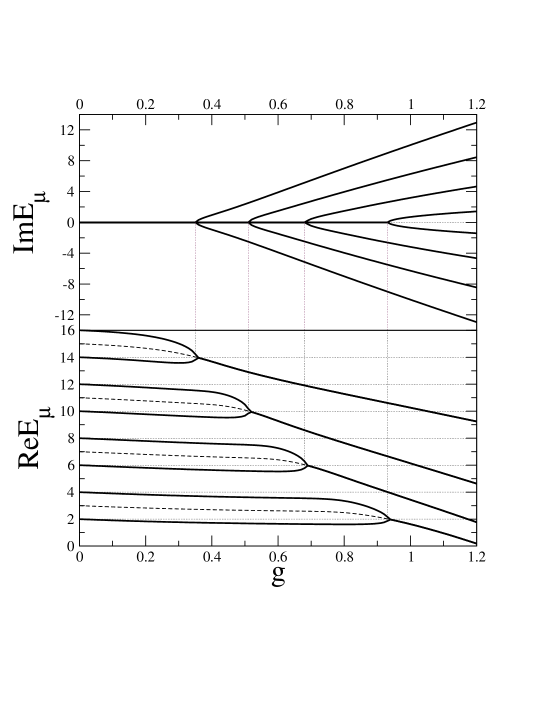
Figure 5: Evolution of the real and imaginary parts of $E_{\mu}(g)$, in units of $d=\omega/N$, for the equally spaced model with $M=N/2=8$, as a function of the coupling constant $g$. For convenience the energy levels are choosen in this figure as $\varepsilon_{j}=2j$. This figure confirms numerically the behaviour found in reference [R-roots, ].

In fig. 5 we plot the real and imaginary parts of $E_{\mu}$, for a system with $M=N/2=8$ pairs. For small values of $g$, all the pair energies are real and below the corresponding energy levels at $g=0$. At a certain value $g_{1}$, the two closest pairs to the Fermi energy, namely $E_{M}$ and $E_{M-1}$, coincide at $\varepsilon_{M-1}$ and then, for larger values of $g>g_{1}$ they form a complex conjugate pair, while the rest of the pair energies remain real. At higher critical values of $g$ the same phenomena happens for the other energies, until all of them become complex. At the critical values of $g$ the Richardson eqs. (6) are singular, but the singularities can be resolved by the change of variables introduced in [R-roots, ].

In fig. 6 we show the distribution of roots for $M=100$ pairs, together with the theoretical curves obtained in section VI, for three different values of $g$. For $g=0.5$ and $1$ there is a fraction of roots which become complex, falling into the arcs $\Gamma$ described by eq. (75), while the real roots extend from the cutting point of the arc $\Gamma$ with the real axis down to the energy $-\omega$. For $g=1.5$ all the roots are complex and fall into the theoretical curve (75). The numerical data are consistent with the value $g_{0}=1.13459$ above which all the energies become complex.

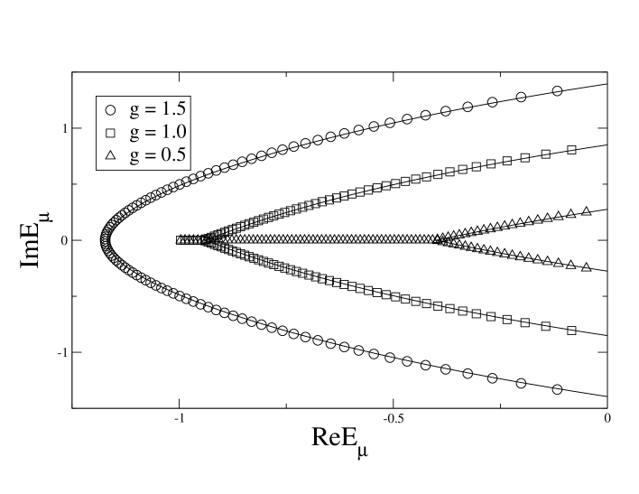
Figure 6: Plot of the roots $E_{\mu}$ for the equally spaced model in the complex $\xi$-plane. The discrete symbols denote the numerical values for $M=100$. The continuous lines are given by eq. (75). All the energies are in units of $\omega$.

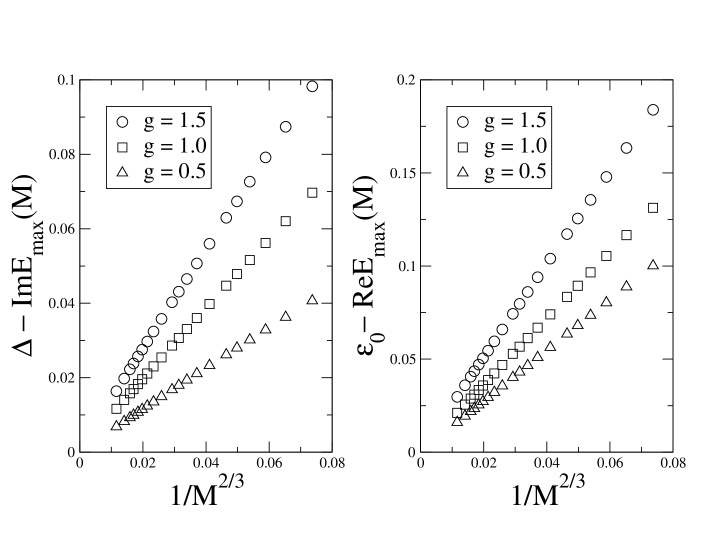
Figure 7: Plots of $\Delta-{\rm Im}\;E_{max}(M)$ and $\varepsilon_{0}-{\rm Re}\;E_{max}(M)$ versus $M^{-2/3}$, for the equally spaced model.

As in the two-level case, the root $E_{max}(M)$ closest to $\varepsilon_{0}+i\Delta$ satisfy the scaling law (84) with an exponent $\theta=2/3$. This result can be proved along the same lines as for the two-level case. In table 2 we give the comparison between the theoretical and numerical values of $\theta$, and in fig. 10 we show the scaling behaviour for three values of $g$.

$\theta$	$g=1.5$	$g=1$	$g=0.5$
analytical	2/3	2/3	2/3
numerical $(\Delta)$	0.646	0.645	0.642
numerical $(\varepsilon_{0}$)	0.658	0.659	0.661

Table 2.- Numerical and analytical values of the exponent $\theta$ appearing in eq. (84) for the equally spaced model. The notation is the same as in table 1.

Figure 8: Density profile of the complex roots for the equally spaced model with $M=800$. Notations are the same as in fig. 3.

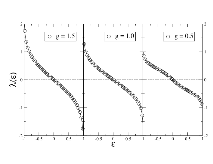
Figure 9: Conserved quantities in the region $\Omega$ in the equally spaced model for $M=20$ and different values of $g$. The continous lines are given by eq. (73).

In fig. 8 we give the fraction of roots per unit length $r(E)/M$ for $M=800$ and three values of $g$. Again, the numerical data fit accurately the theoretical result $r(E)/M=|h(E)|/\pi$, where $h(E)$ is given by eq. (71).

A further check is presented in fig. 9, where the distribution of the conserved quantities $\lambda(\varepsilon_{i})$ for $M=20$ is presented, together with their continuous limit curves given in eq. (73). A very good agreement is achieved even for such a small number of pairs.

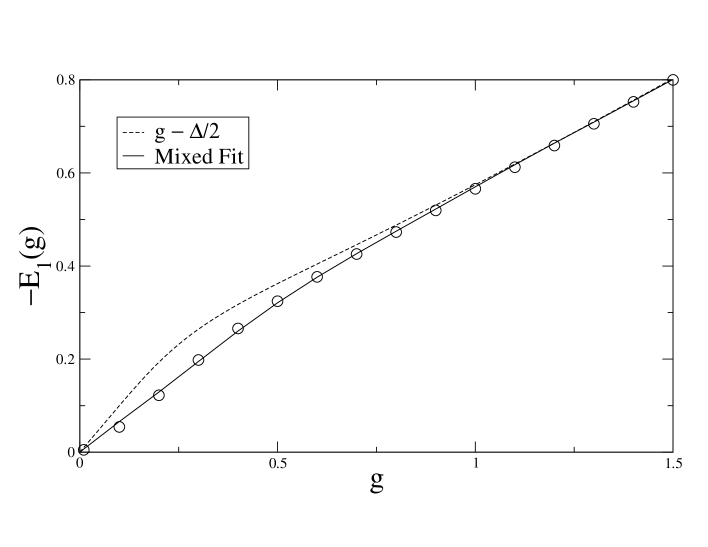
Figure 10: Plot of $-E_{1}(g)$ versus $g$ for the equally spaced level model. The fits of the numerical data are given by eqs. (90) and (LABEL:101) in units of $\omega$.

We have finally studied the condensation energy $E_{C}/M$ as a function of $M$, obtaining the behaviour $E_{C}(M)=e_{\infty}M+E_{1}$, where $E_{1}(g)$ is plotted in fig. 10. An analytic expression for $E_{1}(g)$ is not known R-limit . In order to understand the numerical results we have made two fits. The first one is based on the result obtained for the two-level case, namely

$$-E_{1}(g)=g\omega-\frac{\Delta}{2}\;,$$ (90)

where $\Delta$ is given by eq. (67). Fig. 10 shows that (90) is a good fit for large values of $g$, where all the roots are complex, forming a single arc. For $g\lesssim g_{0}=1.13459$ there is a fraction $M_{complex}/M$ of complex roots, and a fraction $M_{real}/M$ of real roots. This suggests the following mixed fit:

$$-E_{1}(g)/\omega = \left(g-\frac{\Delta}{2\omega}\right)\frac{M_{complex}}{M}+(A+Bg)\;g\;\frac{M_{real}}{M}\;,$$

$$A = 0.6735,\qquad B\ =\ -0.1729,$$

which describes pretty well $E_{1}(g)$ in the whole range of $g^{\prime}s$. In the weak coupling regime there have been proposed several formulas for the finite size corrections of the condensation energy $E_{C}$ using the DMRG method DMRG and the exact solution Sch . In the latter reference it is shown that for couplings $g>g*=1/lnN$, the condensation energy $E_{C}$ can be splitted in two contributions, one due to the complex energy pairs ( the BCS term) and another one due to the real roots ( perturbative term). It would be interesting to clarify the relation between formula (LABEL:101) and eq.(24) in reference Sch .

VIII) Conclusions and prospects

In this paper we have reviewed and completed Gaudin’s continuum limit of the exactly solvable BCS model, and compared its predictions with the numerical solutions describing the ground state of the two-level and the equally spaced models. We have confirmed previously known results R-roots ; random ; vDB1 ; vDB2 , and obtained new ones, which we list below:

• Analytic and numerical determination of the curves $\Gamma$, where the roots $E_{\mu}$ of the Richardson equations lie, together with their density along $\Gamma$. For the equally spaced model the curves $\Gamma$ are given for arbitrary values of the coupling constant $g$, and for the two-level model in the normal regime, i.e. $g<\varepsilon_{1}$, the analytic curves $\Gamma$ differ from those in [G-book, ].

• Analytic expression of the eigenvalues $\lambda_{j}$ of the conserved quantities found by Cambiaggio, Rivas, and Saraceno CRS , which fit accurately the numerical data, even for a few levels.

• Study of the scaling properties of the ground state energy $E(M)$ with the number of pairs $M$ which, in the large $M$ limit, behaves generically as $E(M)=e_{\infty}M+E_{1}+O(1/M)$. For the two-level model, in the superconducting regime, we find an agreement with the analytic result for $E_{1}$ [R-limit, ], while in the normal regime we have guessed an analytic expression for $E_{1}$, which fits perfectly the numerical data. In the critical case there are large deviations in $E(M)$, which can be explained by a term $O(M^{-1/3})$. In the equally spaced model the condensation energy also receives a constant contribution, $E_{1}$, which is fitted with a “phenomenological” formula which combines the effects of the complex and real roots.

• Scaling behaviour of the roots $E_{max}(M)$ which lie closest to the end points of the curves $\Gamma$. This scaling can be characterized by a critical exponent $\theta$, whose analytic values fit well the numerical ones. In the superconducting regimes (i.e. $\forall g>0$ for the equally spaced-model and $g>\varepsilon_{1}$ for the two-level model) we find $\theta=2/3$, while in the normal (critical) regimes of the two-level model we find $\theta=1/2$ ($1/3$). In this manner the exponent $\theta$ characterizes the nature of the ground state. An interesting question is wether $\theta$ shows up in physical observables.

• Generalization of Gaudin’s conformal mapping for the equally spaced model using elliptic functions, which degenerate into trigonometric ones in the limit $\Delta\ll\omega$. This suggest the existence of a rich mathematical structure.

Finally, we shall mention some problems which are worth to investigate along the lines suggested by the present work:

• Study of the excited states and the finite size effects in a more geometrical way, completing the work initiated by Richardson in [R-limit, ].

• Quantum dots at finite temperature is another difficult problem, which has been treated combining several techniques depending on the temperature regime Finite-T ; FFM ; FF . Is it possible to find a thermodynamic Bethe ansatz for this system?

• Study of solutions of Richardson equations with several arcs, i.e. $K>1$ in the notation of section V. For the standard BCS model they must describe very high excited states formed by separate condensates in interaction. This case may be relevant to systems such as arrays of superconducting grains or quantum dots. From a mathematical point of view, the cases with $K>1$ seem to be related to the theory of hyperelliptic curves and higher genus Riemann surfaces, which may shed some light on this physical problem.

• Generalization of Gaudin’s equations to Richardson models based on arbitrary Lie groups ${\cal G}$ AFS . The standard case corresponds to the choice ${\cal G}=SU(2)$. The electrostatic model for generic ${\cal G}$ has charges labelled by vectors of dimension ${\rm rank}\;{\cal G}$. It is naturally to expect that the roots $E_{\mu}^{a}\;(a=1,\dots,{\rm rank}\;{\cal G})$ should fall into several arcs labelled by the index $a=1,\dots,{\rm rank}\;{\cal G}$.

Appendix: Conformal mapping for the equally spaced system

In this appendix we study the analytic structure underlying the shapes of the curves defined by eqs. (74) and (75).

i) Case $\Delta\ll\omega$

In this limit it is convenient to make a conformal mapping G-book from the upper half-plane ${\rm Im}\xi>0$, with a cut in the segment $(0,i\Delta)$, into the half-strip $\lambda>0$, $-\pi/2<\mu<\pi/2$,

$$\xi=i\Delta\;\cosh(\lambda+i\mu).$$ (92)

In the plane $u=\lambda+i\mu$ the curve (74) becomes

$$\lambda\;\tanh\lambda+\mu\;\cot\mu=0.$$ (93)

Figure 11: Half-strip in the $u=\lambda+i\mu$ plane that is conformally equivalent to the upper half $\xi$-plane, with a cut in the interval $[0,\varepsilon_{0}+i\Delta]$. The arcs ${\bf OA}$ and ${\bf OB}$ are given by eq. (93). This figure is borrowed from reference G-book .

Figure 12: Location of the roots $E_{\mu}$ in the $\xi$-plane. The complex roots condense in the arc ${\bf OAO^{\prime}}$, given by eq. (74), while the real ones are distributed in the segment ${\bf X^{\prime}A}$, with a real root between every two energy levels. The point ${\bf A}$ is given by eq. (94). This figure is borrowed from reference G-book .

Figures 11 and 12 show, in the $u$ and $\xi$ planes, the arcs defined by eqs. (93) and (74). The point ${\bf O}$ ($\xi=\varepsilon_{0}+i\Delta)$ is mapped into the origin ($u=0$), where the field $h$ vanishes. In fact $h(\xi)$, as a function of $u$, is simply $h=-2\rho_{0}u$. The point ${\bf O^{\prime}}$ ($\xi=\varepsilon_{0}-i\Delta)$ is the mirror reflection of ${\bf O}$. The arc ${\bf OA}$ is the one that corresponds to the actual numerical solution for ${\rm Im}\xi>0$, while its mirror image, ${\bf O^{\prime}A}$, is the one for ${\rm Im}\xi<0$. We thus see that the whole arc ${\bf OAO^{\prime}}$ cuts the real axis at the point ${\bf A}$ with an energy

$$\varepsilon_{A}=\varepsilon_{0}-\Delta\;\sinh{\lambda_{0}},\qquad\lambda_{0}\;\tanh{\lambda_{0}}=1.$$ (94)

These results are expected from numerical studies, which show that for weak couplings only a fraction of energies $E_{\mu}$ form complex conjugated pairs, which in the limit $N\rightarrow\infty$ organize themselves into arcs, while the other energies remain real and located between the lower energy levels ( see fig. 6). We can check this result computing the number of real and complex roots $E_{\mu}$. From eq. (94) we deduce that the real roots occupy the interval $[-\omega,-\Delta{\rm sinh}\lambda_{0}]$, with a density which is $2\rho_{0}$. Hence the total number, $M_{\rm real}$ of real roots is

$$M_{\rm real}=2\rho_{0}(\omega-\Delta\;\sinh{\lambda_{0}}).$$ (95)

Since the total number of roots is $M=M_{\rm real}+M_{\rm complex}=N/2=2\rho_{0}\omega$, we deduce that

$$M_{\rm complex}=2\Delta\rho_{0}\;\sinh{\lambda_{0}}.$$ (96)

This result agrees with the one obtained integrating the field $h(\xi)$ along the curve $L$ surrounding $\Gamma$ (recall eq. (44)). This integration is more easily done in the $u$-strip

$$M_{\rm complex}=\int_{L}h(\xi)\;d\xi=4\times\int_{0}^{\lambda_{0}+i\pi/2}(-2\rho_{0}u)(i\Delta\sinh{u}\;du),$$ (97)

where the factor 4 comes from the contribution of the up and down, and left and right pieces of the contour $L$. Using contour arguments, it can be shown that the BCS eqs. (43), (44), and (45) also hold in cases where $\Gamma$ cuts the energy interval $\Omega$. As a side comment, we observe that $M_{\rm complex}=\frac{\Delta}{2d}\;{\rm sinh}\lambda_{0}$, agrees with the heuristic argument stating that there are roughly $\Delta_{BCS}/d$ energy levels around the Fermi level that are strongly affected by the pairing interactions T . See also reference Sch for an approximate equation giving the number of complex pairs ( eq. (49)).

ii) Generic case

In order to compare with the numerical results presented in the section VII, it is convenient not to make the approximation $\Delta\ll\omega$. The appropiate change of variables that generalizes (92) is given by

$$\xi=\frac{i\Delta\;\cosh{u}}{\displaystyle{\sqrt{1-\left(\frac{\Delta}{\omega}\;\sinh{u}\right)^{2}}}}\;,$$ (98)

in terms of which $h=-2\rho_{0}u$. The integral $\int h(\xi)d\xi$ can be more easily done in the $u$ plane, yielding for the equation of the curve $\Gamma$

$${\cal R}\left[\frac{i\;u\;\cosh{u}}{\displaystyle{\sqrt{1-\left(\frac{\Delta}{\omega}\;\sinh{u}\right)^{2}}}}-\frac{i\;\omega}{\Delta}\;\arcsin\left(\frac{\Delta}{\omega}\;\sinh{u}\right)\right]=0,$$ (99)

which in the $\xi$-plane gives eq. (75), namely

$${\cal R}\left[i\xi\;\arcsin{\sqrt{\frac{1+\xi^{2}/\Delta^{2}}{1-\xi^{2}/\omega^{2}}}}+\omega\;{\rm Argsinh}{\sqrt{\frac{\Delta^{2}+\xi^{2}}{\omega^{2}-\xi^{2}}}}\right]=0.$$ (100)

In the limit $\Delta\ll\omega$ this equation turns into eq. (74). We can ask when this curve cuts the interval $[-\omega,\omega]$. A convenient parametrization of the cutting point is (recall eq. (94))

$$\xi_{A}=-\frac{\Delta\;\sinh{\lambda_{0}}}{\displaystyle\sqrt{1+\left(\frac{\Delta}{\omega}\;\cosh{\lambda_{0}}\right)^{2}}}\;.$$ (101)

Plugging (101) into (100) we deduce the equation for $\lambda_{0}$,

$$\frac{\lambda_{0}\;\sinh{\lambda_{0}}}{\displaystyle\sqrt{1+\left(\frac{\Delta}{\omega}\;\cosh{\lambda_{0}}\right)^{2}}}=\frac{\omega}{\Delta}\;{\rm Argsinh}\left(\frac{\Delta}{\omega}\;\cosh{\lambda_{0}}\right),$$ (102)

which only has real solutions provided $\Delta\leq\omega$. When $\Delta>\omega$ the arc $\Gamma$ does not touch the interval $[-\omega,\omega]$ and all the roots $E_{\mu}$ are complex. This happens for $g>g_{0}=1.13459$. This value of $g_{0}$ is obtained solving the equation $\sinh{1/g_{0}}=1$.

To complete this appendix we shall show that eq. (98) yields a conformal mapping that generalizes the one found by Gaudin for generic values of $\Delta/\omega$. To do so, let us first perform the change of variables

$$u=i\left(\frac{\pi}{2}-\phi\right),$$ (103)

and introduce the parameters

$$k=\frac{\Delta}{\sqrt{\Delta^{2}+\omega^{2}}},\qquad k^{\prime}=\frac{1}{\sqrt{\Delta^{2}+\omega^{2}}}=\sqrt{1-k^{2}}\,,$$ (104)

in terms of which (98) becomes

$$\xi=\frac{i\Delta k^{\prime}\;\sin{\phi}}{\sqrt{1-k^{2}\;\sin^{2}{\phi}}}\;.$$ (105)

Using the elliptic functions with modulus $k$, and conjugate modulus $k^{\prime}$, we define a new variable $z$ through WW

$$\sin{\phi} = {\rm sn}(z,k),$$

$$\cos{\phi} = {\rm cn}(z,k),$$ (106)

$$\sqrt{1-k^{2}\;\sin^{2}{\phi}} = {\rm dn}(z,k).$$

The relation between $z$ and $\phi$ is given by the equation

$$z(k,\phi)=\int_{0}^{\phi}\frac{d\psi}{\sqrt{1-k^{2}\;\sin^{2}{\psi}}}\;,$$ (107)

while the inverse function is denoted as $\phi={\rm am}\;(z,k)$. The relation between $\xi$ and $z$ reads

$$\xi=i\Delta k^{\prime}\;\frac{{\rm sn}(z,k)}{{\rm dn}(z,k)}\;.$$ (108)

Finally, using the relation ${\rm sn}(K+v,k)/{\rm dn}(K+v,k)={\rm cn}(v,k)/k^{\prime}$, where $K$ is the half-period of the elliptic integrals, eq. (108) turns into

$$\xi=i\Delta\;{\rm cn}(v,k),$$ (109)

where $z=K+v$. The relation between the variables $u$ and $v$ is given by

$$iu=-\frac{\pi}{2}+{\rm am}(K+v,k)=\frac{\pi v}{2K}+\sum_{n=1}^{\infty}\;\frac{2q^{n}}{n(1+q^{2n}}\;\sin{\frac{n\pi(K+v)}{2K}}\;,$$ (110)

where $q=e^{-\pi K^{\prime}/K}$. In the limit $\Delta/\omega\ll 1$ we get $k\rightarrow 0$, $K\rightarrow\pi/2$, and $q\rightarrow 0$, which implies that $iu\rightarrow v$ and eq. (109) reduces to (92).

Figure 13: Graphical representation of the conformal map (109), with the correspondences given in table 3.

Eq. (109) gives a conformal map of the rectangle $-K<{\rm Re}\;v<K,\;0<{\rm Im}\;v<K^{\prime}$ onto the upper half-plane ${\rm Im}\;\xi>0$, with a cut along the linear segment $0<{\rm Im}\;\xi\leq\Delta$ (see reference [N, ] and fig. 13). Some examples of this mapping are given by

$$v=0,\pm K,\pm K+iK^{\prime}\qquad\longrightarrow\qquad\xi=i\Delta,0,\pm\omega\;,$$ (111)

which imply the following identifications between the sides of the rectangle in the $v$-plane and the relevant energy regions in the $\xi$-plane:

cut	$\begin{array}[]{c}{\rm Re}\;\xi=0\\ 0<{\rm Im}\;\xi<\Delta\end{array}$	$\begin{array}[]{c}-K<{\rm Re}\;v<K\\ {\rm Im}\;v=0\end{array}$
lower band	$\begin{array}[]{c}-\omega<{\rm Re}\;\xi<0\\ {\rm Im}\;\xi=0\end{array}$	$\begin{array}[]{c}{\rm Re}\;v=-K\\ 0<{\rm Im}\;v<K^{\prime}\end{array}$
upper band	$\begin{array}[]{c}0<{\rm Re}\;\xi<\omega\\ {\rm Im}\;\xi=0\end{array}$	$\begin{array}[]{c}{\rm Re}\;v=K\\ 0<{\rm Im}\;v<K^{\prime}\end{array}$
off band	$\begin{array}[]{c}|{\rm Re}\;\xi|>\omega\\ {\rm Im}\;\xi=0\end{array}$	$\begin{array}[]{c}-K<{\rm Re}\;v<K\\ {\rm Im}\;v=K^{\prime}\end{array}$

Table 3.- Correspondences of the boundary regions of the conformal map (109).

References

- (1) J. Bardeen, L.N. Cooper and J.R. Schrieffer, Phys. Rev. 108, 1175 (1957).
- (2) R.W. Richardson, Phys. Lett. 3, 277 (1963).
- (3) R.W. Richardson, Phys. Lett. 5, 82 (1963).
- (4) R.W. Richardson and N. Sherman, Nucl. Phys. B 52, (1964) 221.
- (5) R.W. Richardson, J. Math. Phys. 6, 1034 (1965).
- (6) R.W. Richardson, Phys. Rev. 141, 949 (1966).
- (7) R.W. Richardson, J. Math. Phys. 9, 1327 (1968).
- (8) R.W. Richardson, J. Math. Phys. 18, 1802 (1977).
- (9) M. Gaudin, J. Physique 37, 1087 (1976).
- (10) M. Gaudin, “ États propres et valeurs propres de l’Hamiltonien d’appariement”, unpublished Saclay preprint, 1968. Included in Travaux de Michel Gaudin, Modèles exactament résolus, Les Éditions de Physique, France, 1995.
- (11) M.C. Cambiaggio, A.M.F. Rivas and M. Saraceno, Nucl. Phys. A 624, 157 (1997).
- (12) L. Amico, A. Di Lorenzo and A. Osterloh, Phys. Rev. Lett. 86 (2001) 5759.
- (13) J. Dukelsky, C. Esebbag and P. Schuck, Phys. Rev. Lett. 87 (2001) 66403.
- (14) J. Dukelsky and P. Schuck, Phys. Rev. Lett. 86 (2001) 4207.
- (15) J. Dukelsky and S. Pittel, Phy. Rev. Lett. 86 (2001) 4791.
- (16) M. Asorey, F. Falceto and G. Sierra, hep-th/0110266 (to appear in Nucl. Phys. B).
- (17) P. P. Kulish, N. Manojlovic, nlin.SI/0103010.
- (18) H.M. Babujian, J. Phys. A 26, 6981 (1993).
- (19) H.M. Babujian and R. Flume, Mod. Phys. Lett. 9, 2029 (1994).
- (20) G. Sierra, Nucl. Phys. B 572 [FS](2000) 517.
- (21) L. Amico, G. Falci and R. Fazio, J.Phys. A 34 (2001) 6425-6434
- (22) H.-Q. Zhou, J. Links, R.H. McKenzie and M.D. Gould, cond-mat/0106390.
- (23) J. von Delft and R. Poghossian, cond-mat/0106405.
- (24) G. Sierra, “Integrability and Conformal Symmetry in the BCS model”, Proceedings of the NATO Advanced Research Workshop on Statistical Field Theories, Como (Italy), June 2001. Eds. Andrea Cappelli y Giuseppe Mussardo. Kluwer, Academic Publishers (in press). hep-th/0111114.
- (25) G. Sierra, J. Dukelsky, G. G. Dussel, J. von Delft and F. Braun, Phys. Rev. B61, 11890 (2000).
- (26) A. Di Lorenzo, Rosario Fazio, F.W.J. Hekking, G. Falci, A. Mastellone, G. Giaquinta, Phys. Rev. Letters, 84, 550 (2000);
- (27) G. Falci, A. Fubini and A. Mastellone, cond-mat/0110457.
- (28) J. Dukelsky, C. Esebbag and S. Pittel, Phys. Rev. Lett. 88, 062501 (2002).
- (29) J. Hogaasen-Feldman, Nucl. Phys. 28, 258 (1961).
- (30) J. von Delft, Dmitrii S. Golubev, Wolfgang Tichy, Andrei D. Zaikin, Phys. Rev. Lett. 77, 3189 (1996).
- (31) A. Mastellone, G. Falci and R. Fazio, Phys. Rev. Lett. 80, 4542 (1998).
- (32) Fabian Braun, J. von Delft, Phys. Rev. Lett. 81, 4712 (1998).
- (33) J. Dukelsky and G. Sierra, Phys. Rev. Lett. 83, 172 (1999); Phys. Rev. B 61, 12302 (2000).
- (34) M. Schechter, Y. Imry, Y. Levinson and J. von Delft, Phys. Rev. B 63, 214518 (2001).
- (35) J. von Delft and D. C. Ralph, Physics Reports, 345, 61 (2001).
- (36) F. Braun and J. von Delft, Advances in Solid State Physics, vol. 39, p. 341 (Vieweg Braunschweig/Wiesbaden 1999). cond-mat/9907402.
- (37) J. von Delft, F. Braun, in Proceedings of the NATO ASI ”Quantum Mesoscopic Phenomena and Mesoscopic Devices in Microelectronics”, Ankara/Antalya,Turkey, June 1999, Eds. I.O. Kulik and R. Ellialtioglu, Kluwer Ac. Publishers. cond-mat/9911058.
- (38) G. Falci and A. Fubini, cond-mat/0012339;
- (39) M. Tinkham, “Introduction to Superconductivity” (Mc Graw-Hill, 1996), 2nd ed.
- (40) E.T. Whittaker and G.N. Watson, “A course on Modern Analysis”, Cambridge University Press, Cambridge, 1980.
- (41) Z. Nehari, ”Conformal Mapping”, Dover Pub. Inc. New York, 1975.