Geometrical Aspects of Aging and Rejuvenation in the Ising Spin Glass: A Numerical Study

Abstract

We present a comprehensive study of non-equilibrium phenomena in the low temperature phase of the Edwards-Anderson Gaussian spin glass in 3 and 4 spatial dimensions. Many effects can be understood in terms of a time dependent coherence length, $\ell_{T}$, such that length scales smaller that $\ell_{T}$ are equilibrated, whereas larger length scales are essentially frozen. The time and temperature dependence of $\ell_{T}$ is found to be compatible with critical power-law dynamical scaling for small times/high temperatures, crossing over to an activated logarithmic growth for longer times/lower temperatures, in agreement with recent experimental results. The activated regime is governed by a ‘barrier exponent’ $\psi$ which we estimate to be $\psi\sim 1.0$ and $\psi\sim 2.3$ in 3 and 4 dimensions, respectively. We observe for the first time the rejuvenation and memory effects in the four dimensional sample, which, we argue, is unrelated to ‘temperature chaos’. Our discussion in terms of length scales allows us to address several experimentally relevant issues, such as super-aging versus sub-aging effects, the role of a finite cooling rate, or the so-called Kovacs effect.

]

But it’s better to have little free time, then memories don’t intrude. Still, my God, what an amazing phenomenon these memories are.
D. Shostakovich (Letter to I. Glikman).

I Introduction

Spin glasses represent a model system for more ‘complex’ glassy materials. As such, it has attracted a large attention in the last decades [1]. Despite the large number of theoretical, numerical and experimental papers published in the field, the original spin glass problem is still far from being quantitatively understood [2].

Experimental facts that have to be explained are mostly of dynamical nature. The low-temperature dynamics of various spin glass systems has been thoroughly investigated [3, 4], and a number of characteristic features have emerged. Among these are the well-known aging behaviour of the thermoremanent magnetisation or the a.c. susceptibility in isothermal experiments [5], and the spectacular ‘memory’ and ‘rejuvenation’ effects observed in temperature-shifts protocols [6, 7, 8, 9].

It is fair to say that none of the existing theories provides a complete quantitative description of spin glass dynamics [10]. In a recent paper [11], following earlier ideas put forward in the context of the droplet model [12, 13, 14], the notion of separation of length and time scales was argued to be crucial to account for the whole of experimental data. An important ingredient is the existence of a time and temperature dependent coherence length, $\ell_{T}(t_{w})$, such that length scales smaller than $\ell_{T}$ are equilibrated, whereas length scales larger than $\ell_{T}$ are frozen. As a result [11, 12, 13, 14, 15], the aging dynamics after a certain age $t_{w}$ is ascribed to the motion of objects of size $\sim\ell_{T}(t_{w})$. Note that we do not need to specify the topological nature of these objects, postulated to be compact droplets in Ref. [13], but that could be also fractal, sponge-like structures [16, 17, 18]. A simple realization of the above scenario was recently worked out in the context of the 2D XY model [19], suggesting that systems with quasi-long range order [20] have a dynamics very similar to what is observed in spin glass experiments.

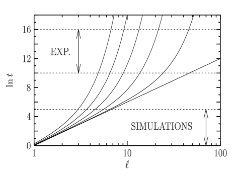
FIG. 1.: Growth law of the coherence length, Eq. (1), for $T/T_{c}=1.0$, 0.9, $\cdots$ 0.5 (from bottom to top). The numerical values are extracted from experiments [11]. The separation of length scales within a given time window is very clear from these curves. Note also the crossover from the critical (power law) regime to the activated regime, where the coherence length is stuck to a value of a few $\xi(T)$.

In this paper, following some previous works [14, 21, 22, 23, 24], we identify a coherence length that grows with the age of the system in the Edwards-Anderson spin glass model [25]. We numerically test the growth law of $\ell_{T}$ proposed in Ref. [11], according to which:

$$t_{w}(\ell_{T})\simeq\tau_{0}\ell_{T}^{z_{c}}\exp\left(\frac{\Upsilon(T)\ell_{T}^{\psi}}{T}\right),$$ (1)

where $z_{c}$ is the dynamical critical exponent, $\psi$ the so-called barrier exponent that describes the growth of the energy barriers with length scales, and $\Upsilon(T)$ a temperature dependent free-energy scale that vanishes at the critical temperature $T_{c}$. This growth law, illustrated in Fig. 1, is motivated both by theoretical considerations [13] and experimental results[11], and was used to analyze further experimental data[26, 27].

By construction, this growth law reduces to usual critical scaling when the barriers on scale $\ell_{T}$ are much smaller than $T$. Assuming that the barrier scale behaves as $\Upsilon(T)=\Upsilon_{0}(1-T/T_{c})^{\psi\nu}$ (where $\nu$ is the correlation length exponent [13], and $\Upsilon_{0}$ an energy scale of order $T_{c}$), the crossover between critical scaling and activated scaling occurs for a dynamical crossover length $\xi(T)$ that diverges at $T_{c}$ as $(1-T/T_{c})^{-\nu}$. Remark that Eq. (1) is obviously not the only possibility to describe this crossover. However, this multiplicative form was found to represent quite accurately the dynamics of the directed polymer or the Sinai model [28, 29], where a similar crossover between diffusive and activated dynamics takes place [30].

As noted in Ref. [11], the growth law Eq. (1) is difficult to distinguish, over a restricted range of length scales, from a pure power law $t_{w}\sim\tau_{0}\ell_{T}^{z}$ with a temperature dependent exponent $z=z(T)>z_{c}$. The latter was previously reported both numerically [14, 22, 23, 24] and experimentally [31]. However, we believe that Eq. (1) should be prefered. One reason is that more elaborated experimental protocols, such as temperature-shift experiments, reveal non-activated effects, as recalled below. This non-activated behaviour is captured by Eq. (1), both through the temperature dependent barrier term $\Upsilon(T)$ and the strong renormalisation of the microscopic time scale by critical fluctuations [11, 26, 27].

The present work is a quantitative investigation of the low-temperature, non-equilibrium dynamics of the Edwards-Anderson spin glass model [25] in finite dimensions, $d=3$ and $d=4$. It can be viewed as the numerical counterpart of Ref. [11]. Here, we take advantage of the fact that simulations, unlike experiments [31], directly give access to $\ell_{T}$, to confirm some of the results obtained in Ref. [11] using indirect evidence. To do so, we perform an extensive series of numerical experiments, including simple aging, temperature-shift and temperature-cycling protocols. We observe for the first time in this system the ‘rejuvenation and memory’ and ‘Kovacs’ effects, which are interpreted using the coherence length $\ell_{T}(t_{w})$. In turn, this allows us to shed new light on several questions such as sub-aging effects, the issue of temperature chaos and the existence of an overlap length, and the very nature of the spin-glass phase. We emphasize also that although simulations and experiments are performed on very different time windows, the length scales probed dynamically are actually not very different, see Fig. 1.

The paper is organized as follows. Section II introduces the model and gives technical details on the simulation. Section III focuses on simple (isothermal) aging. The growth law of the coherence length is studied in section IV. ‘Small’ temperature-shift experiments are performed in section V, while ‘larger’ shifts and cycles are studied in section VI. Physical implications of our results are discussed in section VII, and section VIII summarizes and concludes the paper.

II Model and technical details

We study the Edwards-Anderson spin glass model defined by the Hamiltonian [25]

$$H_{J}[\boldsymbol{s}]=-\sum_{\langle ij\rangle}J_{ij}s_{i}s_{j},$$ (2)

where $\boldsymbol{s}=\{s_{i}\}_{i=1,\cdots,N}$ are $N=L^{d}$ Ising spins located on a 3$d$ or 4$d$ (hyper)cubic lattice of linear size $L$, and $J_{ij}$ are random variables taken from a Gaussian distribution of mean 0 and variance 1. The sum is over nearest neighbors. The spin glass transition is believed [24] to take place at $T_{c}(d=3)=0.95$ and $T_{c}(d=4)=1.8$. In all this paper, the temperature is given in units of the critical temperature, $T/T_{c}(d)\to T$.

To study the aging dynamics, we use a rather large system linear size $L$, $30\leq L\leq 40$ in $d=3$, and $15\leq L\leq 26$ in $d=4$. On the time scale of the simulation, the system never equilibrates on a length scale larger than, say, $\sim 8$ lattice spacings, and we thus always work in the regime $\ell_{T}(t)\ll L$. The dynamics associated to the Hamiltonian (2) is a standard Monte Carlo algorithm, where the spins are randomly sequentially updated. One Monte Carlo step represents $N$ attempts to update a spin.

The behavior of the system is analyzed through the measurements of various physical quantities.

• We compute the energy density, defined by

  $$e=\frac{1}{N}\overline{\langle H_{J}[\boldsymbol{s}]\rangle},$$ (3)

  where $\langle\cdots\rangle$ stands for an average over initial conditions and $\overline{\phantom{|}\cdots\phantom{|}}$ over the disorder.

• We measure the two-time autocorrelation function defined by

  $$C(t_{w}+t,t_{w})=\frac{1}{N}\sum_{i=1}^{N}\overline{\langle s_{i}(t_{w}+t)s_{i}(t_{w})\rangle}.$$ (4)

  We will also consider an a.c. susceptibility like quantity $\chi(\omega,t_{w})$, defined as [14]:

  $$\chi(\omega,t_{w})\equiv\frac{1-C(t_{w}+\frac{1}{\omega},t_{w})}{T}.$$ (5)

• As in previous studies, we extract a coherence length by studying the dynamical 4-point correlation function, defined as

  $$C_{4}(r,t_{w})=\frac{1}{N}\sum_{i=1}^{N}\overline{\langle s_{i}^{a}(t_{w})s_{i+r}^{a}(t_{w})s_{i}^{b}(t_{w})s_{i+r}^{b}(t_{w})\rangle},$$ (6)

  where $(a,b)$ are two copies of the system starting from different initial conditions and evolving with independent thermal histories. This four-point correlation function can be interpreted as the probability that two spins separated by a distance $r$ have the same relative orientation in two independent systems after time $t_{w}$, as is measured by a two-point function in a pure ferromagnet [32].

Our data are typically averaged over 15 (autocorrelation functions, energy density) to 50 (4-point correlation functions) realizations of the disorder. Our data are thus reported without errorbars, which are typically extremely small. Technically, the most difficult part of our work is then to perform a meaningful analysis of the data in order to extract quantitative values of the various physical parameters.

III Isothermal aging: basic facts

In this section, we consider isothermal aging protocols. The system is quenched at initial time $t_{w}=0$ from an infinite temperature to a low temperature $T<1.0$ where it slowly evolves towards its equilibrium state. Although the phenomenology is very-well known [5, 10], and has already been thoroughly investigated in simulations [14, 22, 24, 33], some important points are still poorly understood. We discuss all these aspects in some details in this section. We evaluate, in particular, the implications of Eq. (1) for the theoretical description of the data.

A The spin-spin correlation function: general considerations

As is now well-documented [10], the slow evolution of glassy materials following a quench is best analysed through the measurement of a two-time quantity, typically susceptibility or correlation functions. Here, we measure in the process of isothermal aging the two-time spin-spin correlation function $C(t_{w}+t,t_{w})$ of the system. This quantity can also be accessed experimentally through careful noise measurements [34]. It is represented as a function of the time difference $t$ in Fig. 2 for the 4 dimensional sample. Similar curves are obtained at all temperatures, in $d=3,4$. We get the well-known ‘two-step’ decay of the correlation function with a first, stationary, part followed by a second, non-equilibrium, aging part. The existence of these different regimes is easily understood qualitatively, but a more quantitative description of both time sectors is not completely settled yet.

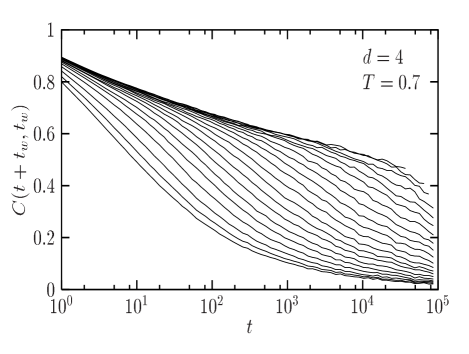
FIG. 2.: Two-time autocorrelation functions $C(t_{w}+t,t_{w})$ in simple aging experiments in $d=4$ and $T=0.7$. We show 20 different waiting times, which are logarithmically spaced in the range $t_{w}\in[2,57797]$ and increase from left to right.

From a theoretical point of view, both mean-field models [35] and the multi-layer trap model [36] predict that the short-time and long-time contributions are additive,

$$C(t_{w}+t,t_{w})\simeq C_{\rm eq}(t)+C_{\rm aging}(t,t_{w}),$$ (7)

whereas aging at a critical point leads to multiplicative scalings [37],

$$C(t_{w}+t,t_{w})\simeq C_{\rm eq}(t)C_{\rm aging}(t,t_{w}).$$ (8)

as used both in simulations [22] and in early analysis of experimental data [4, 38]. The equilibrium part can be fitted, both experimentally and numerically, by a power-law

$$C_{\rm eq}(t)\simeq At^{-x(T)},$$ (9)

with a temperature dependent exponent $x(T)$, which takes rather small values. These two forms (additive and multiplicative) are actually not very different for short times, since $C_{\rm aging}(t,t_{w})$ is approximately constant for $t\ll t_{w}$, in the regime where $C_{\rm eq}(t)$ varies most. However, one should stress that the extrapolation of the multiplicative scaling behavior (8) associated to (9) to large times implies a zero Edwards-Anderson parameter, defined dynamically as:

$$q_{\rm EA}=\lim_{t\to\infty}\lim_{t_{w}\to\infty}C(t_{w}+t,t_{w}).$$ (10)

Indeed, no clear plateau appears in the curves of Fig. 2. On the other hand, the additive scaling suggests a non-zero value of $q_{\rm EA}$, and accounts well for the experimental data [4, 34].

Various scaling forms have been predicted for the aging contribution. In mean-field models, one expects an ‘ultrametric’ behavior [35]

$$C_{\rm aging}(t,t_{w})=\sum_{i}{\cal C}_{i}\left(\frac{h_{i}(t_{w}+t)}{h_{i}(t_{w})}\right),$$ (11)

where the infinite sum over the index ‘$i$’ refers to various ‘time sectors’ [10, 35], and the various functions ${\cal C}_{i}$ and $h_{i}$ have yet unknown functional forms [35]. An explicit example of such a scaling has recently been given in Ref. [39], in the context of the trap model, where the infinite sum boils down to

$$C_{\rm aging}(t,t_{w})={\cal C}\left(\frac{\ln t}{\ln t_{w}}\right).$$ (12)

Note that it is $\ln t$ and not $\ln(t_{w}+t)$ that appears in this equation, which ensures dynamic ultrametricity [39, 40]. This scaling is not observed experimentally, except perhaps for $t\ll t_{w}$ (see Ref. [39]). The scaling (12) is similar to, but different from, the scaling form suggested by the droplet picture, where [13, 41],

$$C_{\rm aging}(t,t_{w})\simeq{\cal C}\left(\frac{\ell_{T}(t+t_{w})}{\ell_{T}(t_{w})}\right),$$ (13)

with $\ell_{T}(t_{w})\sim(\ln t_{w})^{1/\psi}$ [13]. The ‘droplet’ scaling variable $\ln(t+t_{w})/\ln t_{w}$ suggests super-aging, i.e. an effective relaxation time growing faster than the age of the system $t_{w}$, which is not borne out by experimental data showing instead a tendency towards sub-aging. We come back to this point below.

In the absence of any compelling theoretical description, both experiments and simulations have been phenomenologically fitted with some scaling functions of the type

$$C_{\rm aging}(t,t_{w})\simeq{\cal C}\left(\frac{h(t+t_{w})}{h(t_{w})}\right),$$ (14)

where the function $h(u)$ is given various functional forms [10], related to the often debated [4, 42, 43] issue of sub-aging versus super-aging behavior. A widely used form for $h(u)$, which we adopt here, is [4, 44] $h(u)=\exp\left[u^{1-\mu}/(1-\mu)\right]$, where the exponent $\mu$ allows one to interpolate between super-aging ($\mu>1$) and sub-aging ($\mu<1$), via simple aging ($\mu=1$, for which $h(u)=u$). The effective relaxation time is indeed given by $t_{\rm rel}\sim t_{w}^{\mu}$. Note that if one takes $h(u)=\ell_{T}(u)$ with $\ell_{T}$ given by Eq. (1), then, as in the droplet model, super-aging would also be observed for long waiting times, since the effective relaxation time, defined as $h(t_{w})/h^{\prime}(t_{w})$, now grows with the waiting time as

$$t_{\rm rel}(t_{w})\sim t_{w}\left(z_{c}+\frac{\Upsilon(T)\psi\ell_{T}^{\psi}}{T}\right)\gg t_{w},\,\,\,\ell_{T}(t_{w})\gg\xi(T).$$ (15)

Note finally that the existence of a growing coherence length $\ell_{T}(t_{w})$ in spin-glasses does not necessarily implies that the correlation function can be expressed in terms of this length scale only. Indeed, since time scales are broadly distributed, processes corresponding to different lengths scales are expected to mix together. This may also happen in simpler models [43].

B Numerical results

We now discuss our numerical results. We first show in the inset of Fig. 3 (top) that the simple scaling $C(t+t_{w},t_{w})\sim{\cal C}(t/t_{w})$ obviously fails in describing the data. Neither short nor long time scales are correctly described by this form.

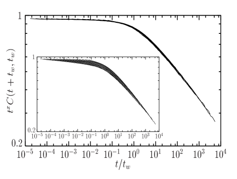
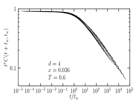
FIG. 3.: Rescaled autocorrelation functions according to the scaling form (8) in $d=3$ (top, $T=0.6$, $x=0.0128$) and $d=4$ (bottom). The inset of the top figure is the simpler scaling form $C(t+t_{w},t_{w})={\cal C}(t/t_{w})$.

We then show in Fig. 3 that when the short-time dynamics is taken into account through the multiplicative scaling form (8), the collapse looks almost perfect in $d=3$ (Fig. 3, top), whereas a small super-aging trend subsists in $d=4$ (Fig. 3, bottom). Indeed, in this $t/t_{w}$ representation, older curves are still above the younger ones, suggesting that rescaling the time by $t_{w}$ is not sufficient to superimpose all the curves. Hence, the introduction of another fitting parameter is required to describe the data, namely the exponent $\mu$ defined above.

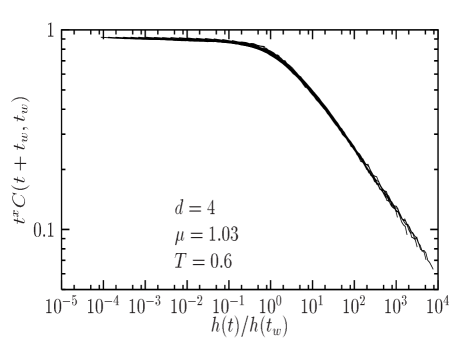
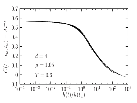
FIG. 4.: Top: Rescaled autocorrelation functions according to the scaling forms (8) and (14), thus allowing for $\mu\neq 1$. Bottom: Rescaled autocorrelation functions according to the scaling forms (7) and (14), choosing parameters so that data extrapolate to a non-zero Edwards-Anderson parameter, as shown by the horizontal dashed line.

We find that with $(x,\mu)$ as free parameters and the multiplicative form (8), the data can be nicely collapsed for the whole temperature range studied, $0.4\leq T\leq 1.0$, in both dimensions $d=3$ and $d=4$. An example of such a rescaling is given in Fig. 4 (top). In $d=3$, our data are consistent with $\mu=1$ in the whole temperature range, and we find an exponent $x(T)$ in close agreement with values reported in Ref. [22]. In $d=4$, our finding for $x(T)$ also follow the reported values [33]. In addition, as suggested by Fig. 3, we find that the exponent $\mu$ has to be larger than 1 for $T\leq 0.6$, while $\mu=1$ is compatible with the data for $0.8\leq T\leq 1.0$. This observation was never reported, although a re-analysis of published data [33] confirms this trend [45]. In both dimensions, we find that the scaling function ${\cal C}(x)$ behaves as ${\cal C}(x)\simeq const$ when $x\ll 1$, and as ${\cal C}(x)\simeq x^{-\lambda}$ for $x\gg 1$, as in Ref. [22].

Close to $T_{c}$ (i.e. $T=1.0$), we find $\mu=1$. This is physically expected, since standard non-equilibrium critical dynamics gives indeed the scaling (8), with $h(t)\sim\ell_{T}(t)\sim t^{1/z_{c}}$. In that case, the coherence length is the usual dynamic correlation length [37, 46, 47]. The fact that the scaling function $h(u)$ changes when the temperature is lowered in $d=4$ suggests that the dynamics leaves the critical regime. It is thus a priori surprising that the multiplicative power-law scaling still holds for low temperatures. The situation appears different in $d=3$, where the dynamics does not show any clear change when the temperature is lowered below $T_{c}$.

One can therefore try to rescale the $4d$ data according to an additive scaling, which allows for a non-zero Edwards-Anderson parameter, Eq. (7). In this case, we have three free parameters, $(x,\mu,A)$, where $A$ is the amplitude of the stationary part $A$. This is unfortunately too much since in this case $A$ (and thus $q_{\rm EA}$) is very poorly constrained. As noted in Ref. [42], the values of the parameters $A$ and $x(T)$ are in fact strongly anti-correlated, but the data is insufficient to pin down their individual values, and hence to conclude on the value of $q_{\rm EA}$. However, noting that $C_{\rm aging}(x)>0,\forall x$ allows us to give a possible range for $q_{\rm EA}$. For instance, for $d=4$ and $T=0.6$, we find that $q_{\rm EA}\in[0.57,0.68]$ leads to a reasonably good rescaling of the data. These values are in agreement with previous estimations of the Edwards-Anderson parameter [33].

Interestingly, the additive procedure has little impact on the value of the aging exponent $\mu$. For $d=3$, we still find that $\mu=1$ allows for a good rescaling of the data, whereas in $d=4$ the super-aging tendency is slightly reinforced by this rescaling. An example of this is shown in Fig. 4 (bottom).

C Conclusion

From the above analysis of our numerical results on isothermal aging, we conclude on the following.

(i) Although data are compatible with the standard scenario where $q_{\rm EA}>0$ for $T<T_{c}$, we cannot rule out, from our numerical study of spin-spin correlation function, the fact that asymptotically $q_{\rm EA}=0$ both in $d=3$ and in $d=4$. Longer simulations in $d=4$ [33] however seem to favor the additive scaling over the multiplicative scaling, and therefore a non-zero Edwards-Anderson parameter.

(ii) The exponent $x$ that describes the short-time decay of the correlation function also describes the behavior of the equilibrium a.c. susceptibility. The measurement of the latter allows then to obtain the value of $x$ independently. It was then shown experimentally that when this is done, the additive scaling (7) works well [4, 38].

(iii) Whatever the chosen rescaling for the short-time dynamics, we find a systematic super-aging behavior in $d=4$. This is consistent with the identification of the scaling function $h(u)$ with a coherence length $\ell_{T}(u)$, growing like Eq. (1). Indeed, the resulting relaxation time given by Eq. (15) can be written approximately as $t_{w}^{\mu}$ with

$$\mu-1=\frac{\psi}{z_{c}}.$$ (16)

On the other hand, no super-aging is found in $d=3$, although, as shown below, Eq. (1) also seems to hold. However the distinction between Eq. (1) and a pure power-law with a temperature dependent exponent will be much harder to establish in $d=3$.

(iv) Our data show no tendency towards sub-aging, in contrast to what is consistently found in all experiments [4]. We shall see below that the introduction of a finite cooling rate (instead of the direct $T=\infty\to T$ quench considered in this section) in fact results in an effective sub-aging.

IV Growth of a coherence length

We now turn to a more geometric characterisation of aging, and try to associate the stationary part of the correlation function to equilibrated small scale dynamics, and the aging part of the correlation function to out-of-equilibrium, large scale dynamics. The time dependent crossover scale is a coherence length, that would be the domain size in a coarsening ferromagnet [32], or the dynamic correlation length at the critical point [46]. In the case of spin-glasses, a more subtle definition is needed [21, 22]. As for the autocorrelation function, we discuss in detail the physics involved in the scaling form of this function. Moreover, we extend previous works in $d=4$ to a larger temperature range. This is necessary in order to extract the parameters involved in Eq. (1). The latter analysis is also new in $d=3$, and allows a direct comparison with experiments.

A The four-point correlation function

1 Definition

As proposed by several authors [21, 22], the coherence length can be measured in a simple isothermal aging protocol from the spatial structure of the 4-point correlation function $C_{4}(r,t)$, defined in Eq. (6). This 4-point function is the analog of the structure factor in a usual domain growth problem [32], adapted to the case of the disordered system under study, where any growing pattern is random and can only be identified by comparing two independent real replicas of the same system, prepared at $t=0$ in a different random state. It measures the similarity of the relative spin orientations in the two systems at a distance $r$ after time $t$. Typical results are presented in Fig. 5. The spatial decay of this correlation function becomes slower when the time increases, clearly indicating the growth of a length scale in the system. This was already noted several times [14, 21, 22, 23].

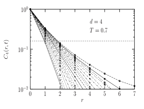
FIG. 5.: 4-point correlation function for $T=0.7$ in $d=4$ measured in an isothermal aging experiment. Times are logarithmically spaced in the range $t_{w}\in[2,57797]$ and increase from left to right. The horizontal dotted line corresponds to $q_{\rm EA}^{2}$, using $q_{\rm EA}=0.4$ from static studies.

2 Functional form of $C_{4}$

The correct identification of the coherence length $\ell_{T}(t_{w})$ is however not completely straightforward. Indeed, the naive definition

$$C_{4}\big{(}r=\ell_{T}(t_{w}),t_{w}\big{)}=c,$$ (17)

where $c$ is an arbitrary constant, say $c=0.1$, leads to inconsistent results, because the decay of $C_{4}$ is not purely (or even possibly stretched) exponential [48]. This fact is very clear in $d=4$, where the definition (17) with $c=0.1$ leads to a coherence length which is such that for some $t_{w}$, $\ell_{T_{1}}(t_{w})>\ell_{T_{2}}(t_{w})$ when $T_{1}<T_{2}$, i.e. a faster growth at lower temperatures. This result is physically unacceptable.

From a more careful analysis of the data [48], one finds that $C_{4}$ receives two contributions: a ‘quasi-equilibrated’ decay for $r<\ell_{T}(t_{w})$, followed by a ‘non-equilibrium’ decay at large distances. This reflects the fact that at time $t_{w}$, the system has equilibrated up to a length scale $\ell_{T}(t_{w})$, with a non trivial equilibrium correlation function. This is the direct analog of the ‘two-step’ behavior observed in the autocorrelation function.

As suggested by previous studies [23, 48], a possible functional form is

$$C_{4}(r,t_{w})=\frac{1}{r^{\alpha(T)}}\,{\cal C}_{4}\left(\frac{r}{\ell_{T}(t_{w})}\right),$$ (18)

with a temperature dependent $\alpha(T)$, and ${\cal C}_{4}(x)$ a scaling function. It is difficult to confirm or dismiss this result, since the numerical correlation functions typically decay over $3-5$ lattice spacings only, and other functional forms are possible (see below). Note that very few equilibrium data is available for this correlation function [49], which would be a very interesting information to compare with Eq. (18).

As noted in Ref. [48], Eq. (18) suggests that $C_{4}(r\to\infty,t_{w}=\infty)$ tends to zero. This must be contrasted with the prediction of the droplet picture or any other theory in which the overlap distribution is a trivial $\delta$-function at $q_{\rm EA}$, where [13]

$$\lim_{r\to\infty}\lim_{t_{w}\to\infty}C_{4}(r,t_{w})=q_{\rm EA}^{2}+O(r^{-\theta}),$$ (19)

where $q_{\rm EA}$ is the Edwards-Anderson parameter and $\theta$ the energy exponent, estimated to be $\sim 0.2$ in $d=3$ [12] and $\sim 0.7$ in $d=4$ [50], i.e., smaller than the values of $\alpha$ reported in Table I below.

Although Fig. 5 suggests that $C_{4}(r,t_{w})$ is rapidly much smaller than $q_{\rm EA}^{2}$, and compatible with $C_{4}(r\to\infty,\infty)=0$, we find that it is still possible to rescale the data according to scaling forms which imply a non-vanishing large distance limit. In order to illustrate this point, we tried the following ansatz (not motivated by any theoretical argument):

$$C_{4}(r,t_{w})=\big{(}q_{\rm EA}^{2}+a\exp(-br)\big{)}\,{\cal C}^{\prime}_{4}\left(\frac{r}{\ell_{T}(t_{w})}\right),$$ (20)

which allows a rescaling of the data as good as Eq. (18). In this case, the stationary part of $C_{4}$ indeed tends towards $q_{\rm EA}^{2}$, but much faster than $r^{-\theta}$. More generally, the inequality $\alpha(T)>\theta$ makes Eq. (19) rather unplausible.

3 Discussion

A word of caution is however needed here. Although a non-zero value of the Edwards-Anderson parameter $q_{\rm EA}$ is expected in the spin-glass phase, dynamical evidence for this is still rather weak, at least in $d=3$. For example, as discussed in the previous section, the dynamic spin-spin correlation function cannot rule out a non-zero value of $q_{\rm EA}$. It is well-known that on the time scale (resp. system size) of dynamic (static) simulations, the apparent value of $q_{\rm EA}$ constantly shifts towards $0$ with increasing times or sizes [24]. In that sense, the evidence that $C_{4}(r,t_{w})$ tends to zero at large distances could be compatible with a very small value of $q_{\rm EA}$. The evidence against the simplest droplet picture is however stronger in $d=4$, since the numerical evidence for $q_{\rm EA}>0$ is more compelling in this case.

An alternative interpretation in three dimensions is that $q_{\rm EA}=0$ at all temperatures, which means that either there is no true spin glass transition, or else that the nature of the spin glass phase is different from what has insofar been theoretically expected. This issue might also be related to the existence of large excitations of finite energy recently found in Ref. [18]. For instance, one could be in a Kosterlitz-Thouless (kt) like situation where $q_{\rm EA}=0$, but the 4-point correlation function changes from exponential for $T>T_{c}$ to power-law for $T<T_{c}$ with, possibly, a temperature dependent exponent $\alpha(T)$. Along this (speculative) line of thought, it has been pointed out recently that the dynamics of a critical phase (such as the kt phase) shares many similarities with spin glass dynamics [19, 47].

B Numerical results for the coherence length

We thus adopt a phenomenological definition of $\ell_{T}(t_{w})$ as the time-dependent length which leads, using Eq. (18), to the best numerical collapse of $C_{4}(r,t_{w})$ measured at different times.

It is important to note that the numerical value of the exponent $\alpha(T)$ used in this scaling plot has a significant influence on the resulting growth law for $\ell_{T}(t_{w})$. Since the spatial support of $C_{4}$ is very small, it is impossible to determine this exponent numerically with great accuracy. The conclusion is that even using the above scaling procedure, there is still some degree of arbitrariness in the definition of the coherence length $\ell_{T}$.

We first report in Table I the values of $\alpha(T)$ found in our simulation for the $d=3$ and $d=4$ cases. Our values for $d=3$ are quite close to the ones found in Ref. [23]. For $d=4$, only the value of $\alpha(T=1.0)=1.63$ has been reported in Ref. [33], in excellent agreement with our determination.

An example of data collapse for the 4-point correlation function can be seen in Fig. 6. As in Ref. [23], we find that the cut-off function ${\cal C}_{4}$ is compatible with a ‘stretched’ exponential form, ${\cal C}_{4}(x)\sim\exp(-x^{\beta})$, but with an exponent $\beta>1$.

$T$	$\alpha(T)$ in $d=3$	$\alpha(T)$ in $d=4$
1.0	0.6	1.63
0.9	0.5	1.35
0.8	0.5	1.25
0.7	0.5	1.0
0.6	0.5	0.9
0.5	0.45	0.9

TABLE I.: Values of the exponent $\alpha(T)$ in $d=3$ and $d=4$. Note that $\alpha(T)$ is nearly constant in $d=3$ but significantly changes with temperature for $d=4$. This will turn out to be important in the following.

The growth of $\ell_{T}(t_{w})$ for different temperatures, $0.5\leq T\leq 1.0$, is reported in $d=3$ and $d=4$ in Fig. 7. From Eq. (1), we expect the coherence length to grow as a power law at short times. This is the critical regime characterized by $\ell_{T}(t_{w})\ll\xi(T)$ such that the growth law is $\ell_{T}(t_{w})\sim t_{w}^{1/z_{c}}$. For larger times, the exponential activated term in Eq. (1) should slow down the growth of $\ell_{T}(t)$ in a temperature dependent manner. The locus of the crossover itself must be temperature dependent. All this is observed numerically, see Fig. 7. This is also qualitatively consistent with the law extracted from experiments [11, 26] and reported in Fig. 1.

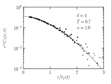
FIG. 6.: Rescaled 4-point correlation function for $T=0.7$ in $d=4$. The full line is a fit of the scaling function ${\cal C}_{4}(x)$ to a ‘stretched’ exponential form, with $\beta=1.7$.

We are now in position to compare the growth law obtained numerically to Eq. (1). The critical exponent $\nu$ is taken from previous numerical work. We take $\nu=1.65$ in $d=3$ and $\nu=0.8$ in $d=4$ [24]. The exponent $z_{c}$ and the microscopic time $\tau_{0}$ are fixed by the data at $T=T_{c}$. We find $z_{c}\sim 7.0$ and $\tau_{0}\sim 2.0$ in $d=3$, $z_{c}\sim 5.9$ and $\tau_{0}\sim 2.2$ in $d=4$. The values for the dynamic exponents are compatible with previous determinations [23, 33].

We are thus left with $\psi$ and $\Upsilon_{0}$ as free parameters. We find that Eq. (1) accounts very well for the data in $d=4$ with $\psi\sim 2.3$ and $\Upsilon_{0}\sim 0.6$, see Fig. 7. In 3 dimensions, we were not able to use Eq. (1) with a fixed $\tau_{0}$. Instead, the fits reported in Fig. 7 give $\psi\sim 1.0$ and $\Upsilon_{0}\sim 5.5$, but were obtained by letting $\tau_{0}$ to be temperature dependent, with a non-monotonic temperature behaviour, for which there is of course no physical explanation. Simpler power law fits with a temperature dependent $z(T)=z_{c}T_{c}/T$ but a constant $\tau_{0}=1$ give equally good results, with much less free parameters. This might indicate:

• either that, as discussed above, the whole Ising spin-glass phase in three dimensions is Kosterlitz-Thouless like, where the dynamics is indeed described by power-laws for all temperatures. This would be compatible with the fact that no cross-over beyond the critical regime is detected in the evolution of $C(t,t_{w})$ and $C_{4}(r,t_{w})$ in $d=3$;

• or that Eq. (1) is too simple to quantitatively reproduce the detailed crossover between critical and activated dynamics in $d=3$. It must be noted that, as emphasized in Refs. [19, 51], the simulations are performed right in the regime where the influence of the critical point is still strong;

• or else that the procedure to extract $\ell_{T}(t_{w})$ from $C_{4}(r,t_{w})$ is somewhat biased.

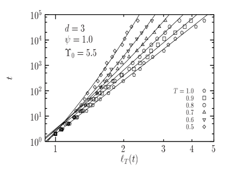
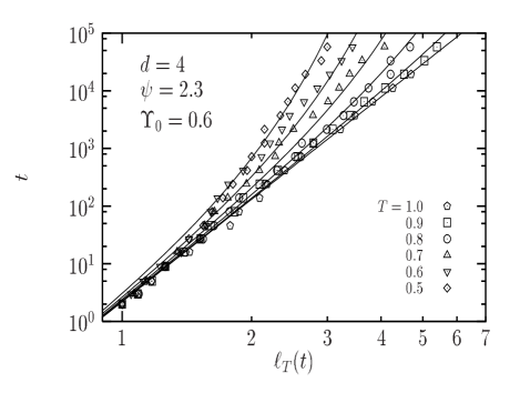
FIG. 7.: Growth laws of the coherence length in 3 dimensions (top) and 4 dimensions (bottom). The points are the data, the full lines are fits to Eq. (1).

We should nevertheless add the following remarks about the three dimensional case.

(i) As will be clear below, the simple power-law growth of $\ell_{T}$ with $z(T)=z_{c}T_{c}/T$ cannot explain the small temperature shift effects, that suggest – both numerically and experimentally – deviations from a pure activated growth.

(ii) One can also extract from the data the local slope of $\log t(\ell_{T})$ as a function of $\log\ell_{T}$, which should be independent of $\ell_{T}$ for a pure power law. One finds instead systematic deviations, such that the effective exponent $z$ indeed increases with $\ell_{T}$, as predicted by Eq. (1). Moreover, the amplitude of these deviations vanish as $T$ increases towards $T_{c}$, in a way very much compatible with Eq. (1).

(iii) Finally, it has been suggested in the past that a pure power-law behaviour for $\ell_{T}(t_{w})$ is associated with ‘Replica Symmetry Breaking’, which predicts that the whole low temperature phase is ‘critical’. We disagree with this point of view: the growth of $\ell_{T}(t_{w})$ could be asymptotically logarithmic, as in the droplet picture, even if the equilibrium phase is not unique. This seems to be two totally separate issues as long as one does not associate $\ell_{T}$ with the size of compact droplets.

V Probing the barriers: Small temperature-shift experiments

In order to directly probe the influence of the barriers on the aging dynamics, we perform numerically the analog of temperature-shift experiments [6]. Similar simulations were already performed in Refs. [14, 52] with qualitative results only. Here we go much further and perform, as was done in Ref. [11], a detailed quantitative analysis of the results. The protocol is the following. The system is quenched from $T=\infty$ to the temperature $T_{1}=T_{2}\pm\Delta T$ where it ages; $\Delta T$ here will always be positive. At time $t_{w}$, the temperature is shifted to $T_{2}$, where the measurements start. We shall discuss the behavior of the autocorrelation function $C(t_{w}+t,t_{w})$.

A Aging is less efficient at lower temperatures

Let us start with the phenomenology. We observe that the decay of the correlation function after the temperature-shift from $T_{1}=T_{2}+\Delta T$ to $T_{2}$ is slower than a purely isothermal aging at $T_{2}$, meaning that preliminary aging at a slightly higher temperature ‘helps’ the system at the final temperature. The opposite effect is found when $T_{1}=T_{2}-\Delta T$, see Fig. 8 (top). In that sense, aging is less efficient at lower temperatures.

Moreover, the decay following the shift has the same functional form, for small enough $\Delta T$, as in a simple aging experiment at temperature $T_{2}$. An example of this feature is shown in Fig. 8. This implies that the correlation function after the shift can be superposed to the correlation obtained in isothermal aging at $T_{2}$ by introducing an effective waiting time. One has $t_{w}^{\rm eff}<t_{w}$ for $T_{2}-\Delta T<T_{2}$. The same effect is observed experimentally when $\Delta T$ is sufficiently small [6].

The determination of the effective age of the sample can be made rather precise when the results of section III are used. The correlation function obtained in the shift experiment for different $\Delta T$ can be collapsed on the master curves of Fig. 4, using $t_{w}^{\rm eff}$ as a single adjustable parameter. This leads to a very precise determination of $t_{w}^{\rm eff}$, which does not require any analytical fit of the data, see Fig. 8.

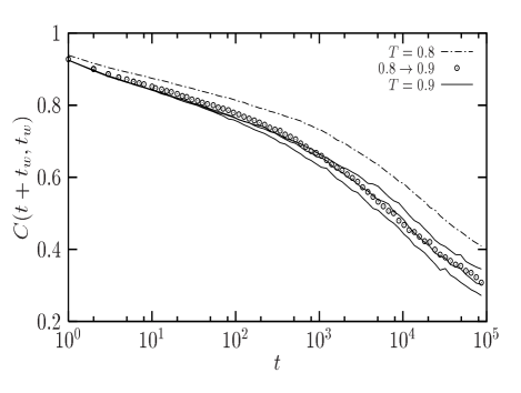
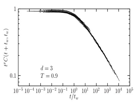
FIG. 8.: Comparison between simple aging and shift experiments in $d=3$. Top: Lines are simple aging curves, $t_{w}=3728$ at $T=0.8$ and $t_{w}=1245$, 2154, and 3728 at $T=0.9$ (from bottom to top). Circles are obtained in the shift $T_{1}=T_{2}-\Delta T=0.8\to T_{2}=0.9$ at time $t_{w}=3728$. One concludes that $1245<t_{w}^{\rm eff}<3728$. Bottom: The correlation obtained in the shift is superposed to the correlation obtained in isothermal aging at $T_{2}$, which gives the value $t_{w}^{\rm eff}=2200$.

B ‘Time is length’: Link with the coherence length

The effective age of the sample may be simply interpreted in terms of length scales. The growth of the coherence length being slower at lower temperatures, one has $\ell_{T_{2}-\Delta T}(t_{w})<\ell_{T_{2}}(t_{w})$. If one assumes that the age of the sample is fully encoded in the value of $\ell_{T}$, then the effective age can be determined by the relation

$$\ell_{T_{2}-\Delta T}(t_{w})=\ell_{T_{2}}(t_{w}^{\rm eff}).$$ (21)

This relation will be correct if $\Delta T$ is not too large, such that quasi-equilibrated structures of sizes $\lesssim\ell_{T_{2}-\Delta T}(t_{w})$ are almost unchanged by the temperature shift. In this case, aging at $T_{2}$ is a simple continuation of aging at $T_{2}-\Delta T$, at a slightly different rate given by Eq. (1).

Figure 9 shows that Eq. (21) works very well. Such a relation was proposed in Ref. [14] assuming a pure power law growth of the coherence length at all temperatures. We show below that our data indeed support Eq. (21), but is incompatible with a pure power law growth of $\ell_{T}$.

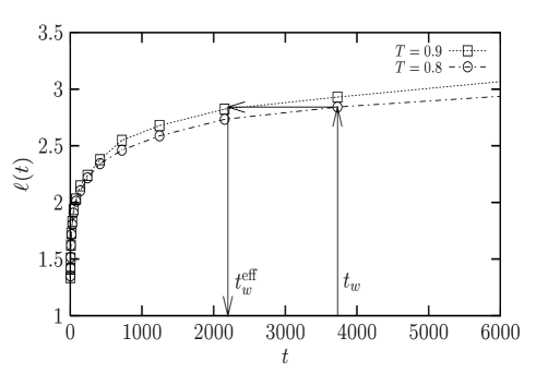
FIG. 9.: This curve shows that the effective age of the system is well described by Eq. (21). The parameters are the same as in Fig. 8.

$T_{2}-\Delta T$	$T_{2}$	$t_{w}$	$t_{w}^{\rm eff}$	$t_{w}^{\rm act}$
0.8	0.9	1245	800	615
0.8	0.9	3728	2200	1629
0.8	0.9	11159	7000	4317
0.7	0.8	1245	650	562
0.7	0.8	3728	2000	1471
0.7	0.8	11159	4600	3839
0.6	0.7	1245	510	503
0.6	0.7	3728	1450	1289
0.6	0.7	11159	3700	3297

TABLE II.: Effective waiting times for various shift-experiments.

Different values of $t_{w}^{\rm eff}$ obtained in a series of shift experiments are reported in Table II. This effective age is also compared to the simple activation prediction, $t_{w}^{\rm act}$, where the same barriers are crossed at the two temperatures. In this case, one gets the prediction that

$$\ln\left(\frac{t_{w}^{\rm act}}{\tau_{0}}\right)=\frac{T_{1}}{T_{2}}\ln\left(\frac{t_{w}}{\tau_{0}}\right).$$ (22)

In this equation, $\tau_{0}$ is the microscopic time that was extracted from the growth of the coherence length at $T=T_{c}$. From Table II, one clearly concludes that $t_{w}^{\rm eff}>t_{w}^{\rm act}$, which suggests that the microscopic ‘trial’ time is actually much larger than $\tau_{0}$. The same systematic effect has been deduced from recent experiments on Ising samples [26].

It is interesting to remark that the simple power law growth $\ell_{T}\sim(t/\tau_{0})^{1/z(T)}$, with $z(T)=z_{c}T_{c}/T$, also leads to the purely activated law Eq. (22) for the effective waiting time, and therefore fails to explain the observed behavior of spin glasses. On the other hand, the mixed critical/activated growth law described in Eq. (1), where the microscopic time $\tau_{0}$ is multiplied by $\ell_{T}^{z_{c}}$, is indeed able to account for deviations from Eq. (22), as already discussed in details in Refs. [2, 26].

We have used the analysis proposed in Ref. [2] to extract $\psi$ and $\Upsilon_{0}$ from the data in Table II. Interestingly, we find $\psi\sim 1.1$, $\Upsilon_{0}\sim 2.1$, compatible with the value obtained from the direct fit of the coherence length. The agreement between direct and indirect determinations of $\psi$ is an important result of this paper, since it validates the analysis performed on experimental data, where no direct determination is possible. However, the value of $\psi=1.0$ favoured by our numerical data is different from the ones reported in previous experimental work on Ising spin-glasses using different procedures: $\psi\sim 0.3-0.5$ [26], $\psi\sim 0.7$ [53], $\psi\sim 1.9$ [27]. It is true that the length scales probed in experiments are at least a factor ten larger than those probed here. This does not explain, however, the scattering of the experimental data.

VI Large temperature shifts: Rejuvenation, Kovacs and memory effects

We turn now to another set of experiments [9], where larger shifts [8] $T_{1}\to T_{2}$, and possibly cycles $T_{1}\to T_{2}\to T_{1}$, are performed. In the previous section, indeed, the dynamics after a shift was the continuation of the aging before the shift. In this section, we use larger temperature shifts, so that the small scale structures that were equilibrated at the first temperature have to adapt to the new one. Precisely how this happens is what we address in this section.

A Is rejuvenation observable in simulations?

The basic message of large temperature shift experiments is that, independently of the sign of $T_{1}-T_{2}$, aging is ‘restarted’ at the new temperature [8]. This ‘rejuvenation effect’ can be nicely observed through the measurement of the magnetic susceptibility $\chi(\omega,t_{w})$. For a given frequency $\omega$, the dominant contribution to the aging part of $\chi(\omega,t_{w})$ comes from the modes with a relaxation time $\sim\omega^{-1}$ which are still out of equilibrium at time $t_{w}$. Rejuvenation after a negative temperature shift comes from fast modes, which were equilibrated at $T_{1}$, but fall out of equilibrium and are slow at $T_{2}$. Therefore, one should expect to see this phenomenon if the equilibrium conformation of length scales $\lesssim\ell_{T_{1}}(t_{w})$ is sufficiently different at the two temperatures (see below for a more precise statement).

This mechanism is qualitatively different from the interpretation involving the notion of temperature chaos [54], and put forward in various approaches [13, 55, 56]. In the latter, the existence of an overlap length $l_{o}(T_{1},T_{2})$, diverging when $T_{2}-T_{1}\to 0$, is postulated. Its physical content is that length scales smaller than $l_{o}$ are essentially unaffected by a temperature shift $T_{1}\to T_{2}$, while larger length scales are completely re-shuffled by the shift. In this picture, rejuvenation is thus attributed to large length scales. Strong rejuvenation effects therefore require a very small $l_{o}$.

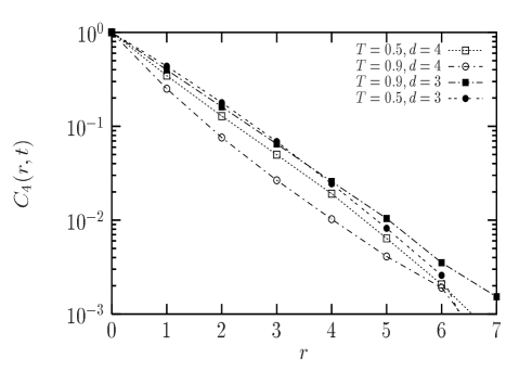
FIG. 10.: The 4-point correlation functions at two temperatures in $d=3$ (black symbols) and $d=4$ (open symbols). Times are chosen so that $\ell_{0.9}\sim\ell_{0.5}$, namely $t(T=0.9)=720$ and $t(T=0.5)=19307$.

It turns out that no clear rejuvenation effects have ever been observed in simulations of the 3 dimensional Ising spin glass [14, 57]. This was first attributed to the fact that $l_{o}(T_{1},T_{2})$ was perhaps numerically large, so that no large scale reorganization could be observed on the time scale of numerical simulations [14]. Another possibility is that the Edwards-Anderson model lacks a crucial ingredient to reproduce the experiments [57], or that the length and time scales involved in the simulations are too small [57].

From the above discussion, we see that the crucial ingredient is the small scale reorganization due to a temperature shift. A natural measure of the spatial organization is provided by the 4-point correlation, Eq. (6). We show in Fig. 10 the function $C_{4}(r,t)$ at two different temperatures $T_{1}=0.9$ and $T_{2}=0.5$ in $d=3$ and $d=4$. Times are chosen so that $\ell_{T_{1}}\sim\ell_{T_{2}}$. It is clear from this Figure that a temperature shift $T_{1}\to T_{2}$ will hardly play any role in $d=3$, whereas the two curves are clearly different in $d=4$. Another way to see this is to observe the temperature dependence of the exponent $\alpha(T)$ reported in Table I. This exponent is almost constant in $d=3$, but varies significantly in $d=4$. This observation suggests that no clear effect can be seen in $d=3$, whereas $d=4$ should be more favourable.

B Negative temperature shifts and rejuvenation

This is indeed what we observe numerically on the analogue of the a.c. susceptibility, defined in Eq. (5). In $d=3$, the amplitude of rejuvenation is very small [14, 57], as expected from the behaviour of the 4-point correlation. In $d=4$, on the other hand, the a.c. susceptibility ‘restarts aging’ after a negative shift $T_{1}\to T_{2}<T_{1}$, at time $t_{s}$, as illustrated in Fig. 11. These curves are very similar to what is observed experimentally.

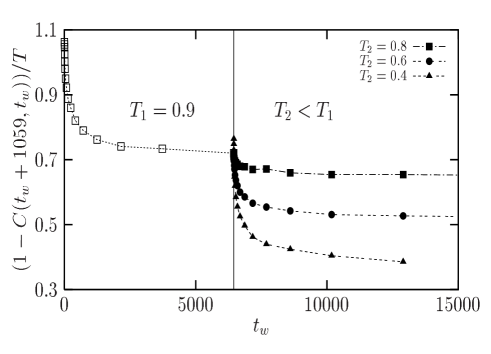
FIG. 11.: Effect of a negative temperature shift on the ‘a.c’ correlation function, for $\omega=1/1059$, after a long stay $t_{s}=6449$ at $T_{1}=0.9$, for different $T_{2}$, in $d=4$. The larger $\Delta T$, the stronger the rejuvenation.

The amplitude of the rejuvenation is found to increase smoothly with the amplitude of the shift $\Delta T=T_{1}-T_{2}$. The ‘temperature chaos’ picture suggests a more brutal crossover: no rejuvenation should appear as long as $l_{o}>\ell_{T_{1}}(t_{s})$. There should thus exists a typical shift-amplitude, $\Delta T^{*}(t_{s})$, such that for $\Delta T<\Delta T^{*}(t_{s})$, rejuvenation should be almost absent. As discussed in section VII B below, we actually can rule out more directly this interpretation in terms of an overlap length.

Although a rather strong rejuvenation appears for large $\Delta T$, one needs to discuss the effect in more details. In particular, the experiments show that for large $\Delta T$, rejuvenation is ‘complete’ in the sense that $\chi(\omega,t_{w})$ after the temperature shift is indistinguishable from the curve obtained after a direct quench from high temperatures. This is closely related to the absence of cooling rate effects on the a.c. susceptibility, as reported in Ref. [7].

We have thus compared the evolution of $\chi(\omega,t_{w})$ from our simulation of a temperature shift to the result obtained after a direct quench. We find that the curves are significantly different. The curve after the shift is clearly ‘older’ than after a direct quench. However, as we discuss in the next section, an experimental quench is never infinitely fast, contrarily to what can be achieved numerically.

C Cooling rate effects and sub-aging

In order to quantify the rejuvenation effect, we investigate the influence of the time $t_{s}$ spent at $T_{1}=0.9$ before the temperature shift. The evolution of $\chi(\omega,t_{w})$ after the shift to $T_{2}=0.5$ for different $t_{s}$ is shown in Fig. 12. We note that as soon as $t_{s}$ is sufficiently long, $t_{s}\gtrsim 240$, the evolution after the shift becomes independent of $t_{s}$. For smaller $t_{s}$, on the other hand, one sees that extra aging contributions are present. Hence, for $t_{s}\gtrsim 240$, some short scale correlations created at $T_{1}$ survive at $T_{2}$, even for large $\Delta T$, making the relaxation different from what it is when $t_{s}=0$. This points towards the absence of temperature chaos and will be discussed further in section VII B. This shows also that for large enough $t_{s}$ the system behaves after the shift as if it had spent an infinite time at $T_{1}$, i.e. as if $t_{s}=\infty$.

The important point now is that experiments always spend some finite time (actually quite long compared to the microscopic time) at all temperatures above the final one $T_{2}$, where some particularly strong correlations very rapidly set in and survive when the temperature is lowered. Therefore, as soon as the cooling rate is not extremely fast, the initial configuration at $T_{2}$ already has some of the correlations that the system wants to grow (see also section VII B). On the other hand, as our simulations show, waiting longer at these intermediate temperatures will not affect further the behaviour at $T_{2}$. The initial age of the system is thus effectively non-zero, but very soon independent of the cooling rate.

Interestingly, this non-zero initial age induces apparent sub-aging effects. Indeed, if $t_{\rm rel}(t_{w})=t_{0}+t_{w}$, where $t_{0}$ approximately accounts for the aging accumulated on the cooling path, the effective exponent $\mu$ is found to be less than unity:

$$\mu=\frac{d\log t_{\rm rel}}{d\log t_{w}}=\frac{1}{1+\frac{t_{0}}{t_{w}}}<1.$$ (23)

We have confirmed this directly on the scaling of the two-time correlation function $C(t+t_{w},t_{w})$ obtained after a slow quench in the $d=4$ case. We find that $\mu=0.96<1$, whereas the scaling obtained after an infinitely fast quench indicated super-aging, $\mu=1.05>1$ (see Fig. 4 above). We believe that this effect is significant. It is thus tempting to ascribe at least part of the sub-aging effects seen experimentally to finite cooling rate effects.

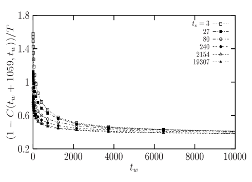
FIG. 12.: Effect of a negative temperature shift on the ‘a.c’ correlation function, after a stay at $T_{1}=0.9$ of various durations $t_{s}$. Final temperature is $T_{2}=0.4$.

D Temperature cycles and memory

Since we have considered above both cases of a positive and a negative temperature cycle, we are now in position to combine both procedures and study temperature-cycles. The experimental procedure is here $T=\infty\to T_{1}\to T_{2}<T_{1}\to T_{1}$. The time spend at $T_{1}$ is $t_{s}$ and the time spent at $T_{2}$ is $t_{s}^{\prime}$. The spectacular ‘memory effect’ arises when the temperature is shifted back to $T_{1}$. It is observed that although aging was fully restarted at $T_{2}$, the system has a strong memory of the previous aging at $T_{1}$. The dynamics at $T_{1}$ proceeds almost as if no cycle to $T_{2}$ had been performed [9]. The coexistence of rejuvenation and memory was made more spectacular in the ‘dip-experiment’ proposed in Ref. [7]. This protocol is too complicated to be studied theoretically, but basically carries the same physical content as the cycle we discuss here.

As discussed in [2, 11] the memory effect is a simple consequence of the separation of time and length scales. When the system is at $T_{2}<T_{1}$, rejuvenation involves very small length scales as compared to the length scales involved in the aging at $T_{1}$. Thus, when the temperature is shifted back to $T_{1}$, the correlations of length scale $\ell_{T_{2}}(t_{s}^{\prime})$ grown at $T_{2}$ almost instantaneously re-equilibrate at $T_{1}$ (in fact in a ‘memory’ time scale $t_{m}$ such that $\ell_{T_{1}}(t_{m})\sim\ell_{T_{2}}(t_{s}^{\prime})$, which implies that $t_{m}\ll t_{s}^{\prime}$ when $\Delta T$ is sufficiently large). The memory is thus stored in the intermediate length scales, between $\ell_{T_{2}}(t_{s}^{\prime})$ and $\ell_{T_{1}}(t_{s})$.

Hence, the explanation of the memory effect relies on the separation of length scales only. This ingredient is distinct from the one needed to observe rejuvenation, which relies on the reorganization of small length scales after a temperature change. Since we have shown that these two ingredients are present in the 4 dimensional spin glass, we are able to reproduce experimental data very well in Fig. 13, where, for purely esthetic reasons, a double cycle was performed.

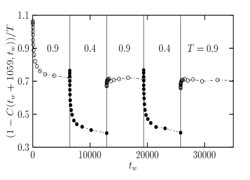
FIG. 13.: Evolution of the ‘a.c.’ correlation function in the procedure $T=\infty\to T_{1}=0.9\to T_{2}=0.4\to T_{1}\to T_{2}$, showing, as in experiments the coexistence of rejuvenation and memory effects.

E Positive temperature shifts

From the results of the previous sections, the physics in a shift experiment is the following. At the first temperature $T_{1}$, the system evolves towards equilibrium through the growth of a coherence length $\ell_{T_{1}}$. When the temperature is shifted to $T_{2}$ at time $t_{s}$, all length scales are driven out of equilibrium. Length scales smaller than $\ell_{T_{1}}(t_{s})$ undergo a ‘quench’ from $T_{1}$ to $T_{2}$, while larger length scales which were not equilibrated at $T_{1}$ undergo a quench from $T=\infty$ to $T_{2}$. If $T_{2}<T_{1}$, then larger length scales do not matter due to the huge separation of time scales.

The situation is different in a shift such that $T_{2}>T_{1}$. Then small length scales have to ‘unfreeze’ to find their new equilibrium at $T_{2}$, while larger ones which where frozen at $T_{2}$ grow as if the quench had been from $T=\infty$.

To support further this physical picture, we performed a positive temperature shift experiment $T_{1}=0.5\to T_{2}=0.9$, after time $t_{s}=19307$ at $T_{1}$, and then some extra time $t$ at $T_{2}$. The results are described in Fig. 14 which shows both the behavior of the autocorrelation and the 4-point correlation after the shift.

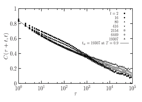
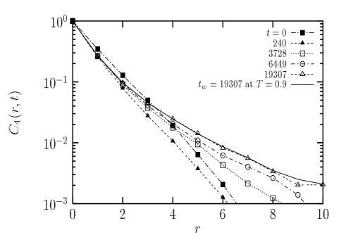
FIG. 14.: Autocorrelation function (top) and spatial correlation function (bottom) in a positive cycle $T_{1}=0.5\to T_{2}=0.9$. Times $t$ refer to time spent after the shift. For comparison, full lines show curves obtained in a direct quench to $T_{2}$. Small and large scales behave very differently. Note also the similarity between both figures which makes clear the link between time and length.

Let us comment first on the time correlation functions, Fig. 14 (top). Immediately after the shift, $t=0$, the decay of the correlation shows a short-time part which is slower than the reference curve with $t_{w}=19307$ at $T_{2}$, and a long-time part which is faster. This nicely illustrates the two types of structures present at that time in the system.

Then, small scale structures very rapidly equilibrate at the new temperature, $t\leq 416$. Note that it took $t_{s}=19307$ to reach the same coherence length at $T_{1}$, a consequence of the length scale separation. After this short transient, dynamics proceeds as if the initial stay at $T_{1}$ was not present, and the subsequent aging is very similar to isothermal aging at $T_{2}$, as soon as $t\geq 2154$. The same features are also clearly visible on the 4-point correlation function, see Fig. 14 (bottom). Note in particular how small scales rapidly ‘unfreeze’ before the large scales evolve towards equilibrium: the correlation for $t=240$ is below the one for $t=0$, before the coherence length $\ell_{T_{2}}(t)$ grows beyond $\ell_{T_{1}}(t_{s})$.

F The ‘Kovacs effect’

This dual behavior between small and large length scales results in a spectacular effect, which was first observed by Kovacs in polymeric glasses [58]. Further developments may be found in Refs. [44, 59]. Since it is referred to in the literature as a ‘memory effect’, but is different from what the spin glass literature names ‘memory’ (see above), we shall follow Ref. [19] and describe this as the ‘Kovacs effect’.

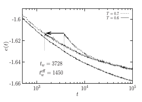
FIG. 15.: Behavior of the energy density in a shift experiment from $T_{1}=0.6$ to $T_{2}=0.7$, at time $t_{w}=3728$, compared with its decay in simple aging experiments (lines), in $d=3$. A simple shift with $t_{w}^{\rm eff}=1450$ allows one to superimpose the curves.

We focus here on the energy density $e(t)$ after a positive temperature shift. The Kovacs effect concerns the specific volume, but the difference is irrelevant for our purposes. Like in recent numerical experiments [14], we find that the decay of the energy density following the shift follows the same time evolution as in the simple aging case, if an appropriate effective waiting time $t_{w}^{\rm eff}$ is properly taken into account, see Fig. 15. We find that the effective age of the sample defined from the correlation function or from Eq. (21) works well for the energy density also. This is illustrated in Fig. 15.

Kovacs [58] noticed that in a similar protocol on polymer glasses, the same non-monotonic initial behavior could be seen in the evolution of the specific volume as we observe in Fig. 15 for the energy density of the spin glass immediately after the shift. Zooming on the transient region and setting the origin of time when the temperature is shifted leads to the curves plotted in Fig. 16. The top curves of Fig. 16 are specially designed to follow Kovacs’ experiments, where the time $t_{s}$ of the shift is chosen so that $e_{T_{1}}(t_{s})=e_{T_{2}}(t=\infty)$. Since the energy density has already the correct equilibrium value at the new temperature, the naive expectation is that $e(t>t_{s})=const$. Instead, the non-monotonic behavior of Figs. 16 is observed.

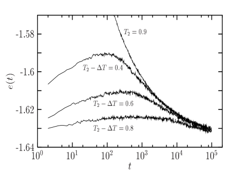
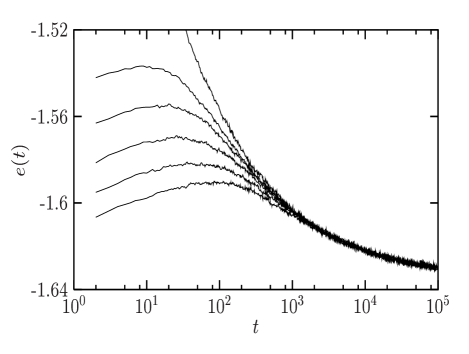
FIG. 16.: Non-monotonic behavior of the energy in a shift experiment. Top: Same $T_{2}$ but different $\Delta T$. Waiting times are such that the energy just before the shift is $\sim e_{\rm eq}(T_{2})$ as in experiments on polymeric glasses. Bottom: The $\Delta T$ is the same in all shifts, but shift times are different, $t_{s}=57797$, 19307, 6449, 2154, 720 and $t_{s}=0$ (from bottom to top).

The presence of a growing coherence length allows one to give a very simple interpretation of this ‘Kovacs effect’ [19]. It results indeed precisely from the dual behavior of length scales described above. When the temperature is shifted to $T_{2}$, length scales shorter than $\ell_{T_{1}}(t_{s})$ have to re-equilibrate at $T_{2}$, where their equilibrium energy is higher than at $T_{1}$. This explains the initial rise of $e(t_{s}+t)$. On the other hand, length scales larger than $\ell_{T_{1}}(t_{s})$ still have to ‘cool down’ and decrease their energy. These two opposite trends directly explain the ‘Kovacs effect’. This scenario was recently illustrated on the exactly soluble example the 2D XY model [19].

It is possible to be more quantitative here, using the coherence length as an ingredient [19]. The time scale $t_{K}$ where the energy density reaches its maximum corresponds in this picture to the time where small length scales have re-equilibrated at the new temperature. Hence, an excellent approximation for this time scale should be:

$$\ell_{T_{2}}(t_{K})\sim\ell_{T_{1}}(t_{s}).$$ (24)

This relation says that $t_{K}$ is an increasing function of $t_{s}$, and a decreasing function of the temperature difference, as is obvious from Figs. 16. The height $e_{K}$ of Kovacs’ hump varies in the opposite direction, as expected from the inverse power-law dependence of the excess energy with the coherence length, $e_{K}\sim\ell_{T_{2}}(t_{K})^{\theta-d}$, found in Ref. [14]. We numerically find that all the curves of Figs. 16 can actually be collapsed into a single master-curve (see Fig. 17) which thus takes the form:

$$e(t+t_{s})\simeq e_{\rm eq}(T_{2})+e_{K}f\left(\frac{t}{t_{K}}\right),$$ (25)

where the scaling function $f(x)$ behaves approximately as a power law for large arguments.

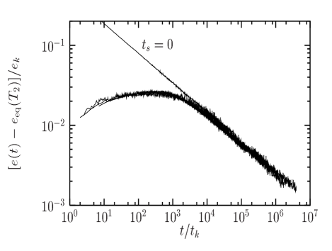
FIG. 17.: All the curves of Fig. 16 are superposed using Eq. (25). The curve ‘$t_{s}=0$’ refers to a direct quench to $T_{2}$.

VII Physical Discussion

A Physical picture of the spin-glass phase

Mean-field theories have nothing to say about possible relevant length scales (such as $\ell_{T}$) and their time and temperature dependence. On the other hand, the droplet picture, which focuses on relevant length scales, seems to miss some important points such as the power-law behaviour of the 4-point correlation function. This point is important since it allowed us to account for rejuvenation effects without the need of the concept of temperature chaos.

One interpretation of the above results is that, as predicted by mean-field theories and given some credit by recent numerical work on low-lying excitations [16, 17], different equilibrium configurations are accessible to the spin-glass in its low temperature phase. These configurations have a global overlap which is close to zero, but can be locally similar. The fact that the stationary part of $C_{4}(r,t)$ decays as a power-law suggest the existence of a fractal ‘backbone’ of spins that have identical mutual orientations for all these configurations, with a fractal dimension $d_{f}=d-\alpha$. It is reasonable to assume that the small scale properties of this backbone will be temperature dependent: more spins will freeze and join the backbone as the temperature is reduced. The simplest scenario compatible with a zero minimal overlap is that the backbone is dense on small scales, and fractal on large scales, with a temperature dependent crossover length $\ell^{*}(T)$. The effective exponent $\alpha(T)$ would in this case decrease with temperature, as seen numerically. Another possibility is that the fractal dimension (and thus the exponent $\alpha$) is truly temperature dependent, as in the low temperature phase of the 2D XY model. As discussed above, there are actually many phenomenological similarities between the spin-glass phase and the 2D XY model, provided length scales, rather than time scales, are compared [19, 47].

The power-law decay of $C_{4}(r,t)$ suggests that the whole spin-glass phase is in a certain sense critical, at least in the ‘zero-overlap’ sector which was indeed found to be mass-less in replica field analysis [60]. However, this is not in contradiction with the existence of a finite correlation length $\xi(T)$ separating critical from activated dynamics within a single ‘state’. A pure power-law growth of $\ell_{T}$ is not necessarily a consequence of the criticality of the spin-glass phase.

Of course, the numerical evidence for this scenario is fragile, and it could be that $C_{4}(r,t\to\infty)$ in fact tends for large $r$ towards $q_{\rm EA}^{2}$. For the purpose of interpreting aging experiments, however, it is sufficient that this scenario holds even approximately on the relevant time and length scales.

B Rejuvenation from small scales and absence of temperature chaos

The role of temperature changes can be exactly computed in the Random Energy Model [61] and in the critical phase of the XY model [19]. Both show that it is possible to induce strong rejuvenation effect without the existence of an overlap length. Several facts, reviewed in Ref. [11], also suggest that the overlap length is not relevant to the experimental findings. Here, we want to address this question more precisely on the basis of numerical results. As shown above, we can now observe beyond any doubts rejuvenation (and memory) effects in the $d=4$ Edwards-Anderson model which are very similar to those observed experimentally. We have also investigated directly the way configurations evolve during a temperature shift using a mixed 4-point correlation function, defined as follows:

$$C_{4}(r,\ell,T_{1},\Delta T)=\frac{1}{N}\sum_{i=1}^{N}\overline{\langle s_{i}^{a}(t_{w})s_{i+r}^{a}(t_{w})s_{i}^{b}(t_{w}^{\prime})s_{i+r}^{b}(t_{w}^{\prime})\rangle},$$ (26)

where replica $a$ is at temperature $T_{1}$, replica $b$ at temperature $T_{2}=T_{1}-\Delta T$, and the times $t_{w}$, $t_{w}^{\prime}$ are chosen such that the coherence length is equal to a common value $\ell$ at the two temperatures. Obviously, when $\Delta T=0$, this correlation function is identical to the previous one. For $\Delta T>0$, this correlation function measures the similarity between the patterns grown at the two different temperatures. In a temperature chaos scenario, one expects the following inequality:

$$C_{4}(r,\ell,T_{1},\Delta T)\leq C_{4}(r,\ell,T_{1},\Delta T=0).$$ (27)

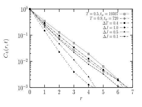
FIG. 18.: Mixed correlation functions, both for temperature changes and for coupling changes (black symbols), compared to standard four-point functions (open symbols). It is clear that the two perturbations ($\Delta T$, $\Delta J$) have qualitatively different effects.

Figure 18 shows that this is not the case. The results are actually compatible with the idea that the same patterns grow at the two temperatures – the backbone supporting the common parts of these patterns being more fluffy at lower temperatures. This conclusion was already reached above when we discussed cooling rate effects.

An interesting comparison can be made with a situation where chaos is expected, e.g. when the couplings are changed [54]. We therefore also show in the same figure the mixed correlation function when the couplings are changed between replica $a$ and replica $b$ according to:

$$J_{ij}\longrightarrow\frac{J_{ij}+\Delta J_{ij}}{\sqrt{1+\Delta J^{2}}},$$ (28)

where $\Delta J_{ij}$ are independent Gaussian variable of variance $\Delta J^{2}$ and mean 0. In this case, the inequality (27) is indeed clearly observed. We conclude thus that $\Delta T$ and $\Delta J$ have a qualitatively different influence on the system.

Note that our mixed correlation function, once integrated over space, leads to the overlap between the two temperatures. The latter quantity was studied directly in Ref. [62] in $d=3$, with conclusions similar to ours.

The simultaneous observation of rejuvenation and absence of temperature chaos is an important result of this paper. In $d=3$, no temperature chaos was found, but no rejuvenation either. This left the door open to the possibility that the length scales investigated were too small to observe these two effects. We have thus demonstrated that both issues can be separated. Of course temperature chaos on large length scales is still possible, but is not needed to interpret rejuvenation effects.

In summary, our results confirm that rejuvenation is due to the freezing of small length scale modes which were ‘fast’ at the higher temperature. This freezing changes the correlations on small scales, as seen on the 4-point correlation function. This is in agreement with the scenario based on a hierarchy of length scales proposed in Ref. [2, 11], and with the phenomenology of the XY model [19], and is markedly different from the temperature chaos picture. This feature can be illustrated in the 2D XY model [63], where each Fourier mode $\varphi(q)$ of the order parameter is affected by a temperature shift. In the spin-wave approximation, one has $\langle\varphi(q)\rangle\sim T/q^{2}$. Hence, each mode is affected when the temperature is changed by $\Delta T$ by an amount

$$\delta\langle\varphi(q)\rangle\sim\frac{\Delta T}{q^{2}},$$ (29)

which shows that larger length scales are more influenced, but with no typical ‘overlap length’.

VIII Summary and conclusion

The interest of a long paper is that a detailed discussion of rather subtle points can be given. The drawback, obviously, is that the message is somewhat diluted. We therefore give in this last section the main conclusions from our study and end on open problems.

• Aging dynamics in spin-glasses can be associated with the growth of a coherence length $\ell_{T}$, separating small, equilibrated scales $<\ell_{T}$ from large frozen, out of equilibrium scales $>\ell_{T}$. This scale is however not a domain size in the usual sense, but rather the size of a backbone of spins common to all spin-glass configurations. This interpretation stems from the power-law decay of the 4-point correlation function from which $\ell_{T}$ is extracted.

• The coherence length $\ell_{T}$ follows a critical power-law growth at small times that becomes activated for larger times, and is well described by Eq. (1). The associated barriers $\Upsilon(T)$ vanish at the critical temperature. The barrier exponent $\psi$ was estimated to be $\psi\sim 1.0$ for $d=3$ and $\psi\sim 2.3$ in $d=4$.

• This mixed critical/activated growth law allows one to interpret several important aspects of both simulations and experiments, for example the deviations from a purely activated behaviour that are revealed by temperature shift procedures, or the super-aging behaviour of the correlation function observed in $d=4$.

• The short scale behaviour of the 4-point correlation is quite sensitive to temperature in $d=4$, but much less in $d=3$. This in turn leads to strong rejuvenation effects in $d=4$, quite similar to those observed in experiments, that we observe for the first time in simulations.

• An interpretation of the observed rejuvenation in terms of temperature chaos is, we believe, ruled out: see Fig. (18). Rather, some correlations built at a higher temperature persist and are reinforced at lower temperatures.

• A finite cooling rate effect follows from this, which, interestingly, leads to an apparent sub-aging behaviour for the correlation function, instead of the super-aging that holds for an infinitely fast quench. The cooling rate dependence however saturates quickly as soon as the cooling rate is not infinitely fast. Both these features agree with experiments, for which the cooling rate is always very slow compared to microscopic frequencies.

• The dichotomy between small, equilibrated scales and large, frozen scales allows one to account semi-quantitatively for many features, such as the role of temperature shifts, the memory effect or the Kovacs’ hump.

Although our results are suggestive, several unsettled points remain. In particular, rejuvenation effects are found in $d=4$, but not in $d=3$, whereas experiments are obviously performed in $d=3$. We conjecture that for the time scales investigated, the large scale topology of space is irrelevant, and the major difference between $d=3$ and $d=4$ should rather come from the local connectivity. Hence it should be possible to obtain rejuvenation in a $d=3$ model with more neighbours, and reproduce most experimental results with a realistic model.

The most important theoretical point is obviously the nature of the spin-glass phase. A well posed problem (but very difficult to settle numerically) is the true long distance behaviour of the 4-point correlation function: power-law decay, as expected from replica symmetry breaking theories, or convergence towards $q_{EA}^{2}$, as for a disguised ferromagnet? The final picture of real spin-glasses might in the end have borrow concepts from both theories. The hope is that the concepts that will emerge will be useful to understand many other glassy systems, which share a very similar phenomenology.

Note added

After this manuscript appeared as a preprint (condmat/0202069), a paper by Yoshino et al. (cond-mat/0203267) appeared where the dynamics of 4-d EA model is studied, and the results also interpreted as a crossover between critical and activated dynamics. The value of the exponents $z_{c}$ and $\psi$ given in that paper slightly differ from those obtained here. For example, $\psi$ is found to be in the range $2.5-3$ whereas we report $\psi\sim 2.3$. One possible explanation is that the procedure to extract $\ell_{T}(t_{w})$ form $C_{4}(r,t_{w})$ is quite different.

REFERENCES

- [1] Spin Glasses and Random Fields, Ed.: A. P. Young (World Scientific, Singapore, 1997).
- [2] J.-P. Bouchaud, in Soft and fragile matter, Eds.: M. E. Cates and M. R. Evans (Institute of Physics Publishing, Bristol, 2000).
- [3] P. Nordblad and P. Svedlindh, in Ref. [1].
- [4] E. Vincent, J. Hammann, M. Ocio, J.-P. Bouchaud and L. F. Cugliandolo, in Complex behavior of glassy systems, Ed.: M. Rubi Springer Verlag Lecture Notes in Physics, vol. 492 (Springer Verlag, Berlin, 1997). See also cond-mat/9607224.
- [5] L. Lundgren, P. Svedlindh, P. Nordblad and O. Beckman, Phys. Rev. Lett. 51, 911 (1983).
- [6] J. Hammann, M. Lederman, M.Ocio, R. Orbach and E. Vincent, Physica A 185, 278 (1992).
- [7] K. Jonason, E. Vincent, J. Hammann, J.-P. Bouchaud and P. Nordblad, Phys. Rev. Lett. 81, 3243 (1998).
- [8] L. Lungren, P. Svelindh, and O. Beckman, J. of Magn. Magn. Mater. 31-34, 1349 (1983).
- [9] P. Réfrégier, E. Vincent, J. Hammann, and M. Ocio, J. Phys. (France) 48, 1533 (1987).
- [10] J.-P. Bouchaud, L. F. Cugliandolo, J. Kurchan and M. Mézard, in Ref. [1].
- [11] J.-P. Bouchaud, V. Dupuis, J. Hammann and E. Vincent, Phys. Rev. B 65, 024439 (2001).
- [12] A. J. Bray and M. A. Moore, J. Phys. C 17, L463 (1984); and in Heidelberg Colloquim on Glassy Dynamics, Lectures Notes in Physics 275, Eds.: J. L. van Hemmen and I. Morgenstern (Springer, Berlin, 1987).
- [13] D. S. Fisher and D. A. Huse, Phys. Rev. B 38, 373 (1988).
- [14] T. Komori, H. Yoshino and H. Takayama, J. Phys. Soc. Jpn. 68, 3387 (1999); 69, 1192 (2000); 69, Suppl. A 228 (2000); K. Hukushima, H. Yoshino, and H. Takayama, Prog. Theor. Phys. Supp. 138, 568 (2000).
- [15] A. Barrat and L. Berthier, Phys. Rev. Lett. 87, 087204 (2001).
- [16] F. Krzakala and O. C. Martin, Phys. Rev. Lett. 85, 3013 (2000).
- [17] M. Palassini and A. P. Young, Phys. Rev. Lett. 85, 3017 (2000).
- [18] J. Lamarcq, J.-P. Bouchaud, O. C. Martin and M. Mézard, preprint cond-mat/0107544.
- [19] L. Berthier and P. C. W. Holdsworth, Europhys. Lett. 58, 35 (2002).
- [20] D. E. Feldman, Int. J. Mod. Phys. B 15, 2945 (2001).
- [21] D. A. Huse, Phys. Rev. B 43, 8673 (1991).
- [22] J. Kisker, L. Santen, M. Schreckenberg, and H. Rieger, Phys. Rev. B 53, 6418 (1996).
- [23] E. Marinari, G. Parisi, F. Ricci-Tersenghi, J. J. Ruiz-Lorenzo, J. Phys. A 33, 2373 (2000).
- [24] E. Marinari, G. Parisi and J. J. Ruiz-Lorenzo in Ref. [1].
- [25] S. F. Edwards and P. W. Anderson, J. Phys. F 5 965 (1975).
- [26] V. Dupuis, E. Vincent, J.-P. Bouchaud, J. Hammann, A. Ito and H. A. Katori, Phys. Rev. B 64, 174204 (2001).
- [27] P. E. Jönsson, H. Yoshino, P. Nordblad, H. Aruga Katori, and A. Ito, preprint cond-mat/0112389.
- [28] H. Yoshino, unpublished.
- [29] M. Sales, J.-P. Bouchaud and F. Ritort, in preparation.
- [30] J.-P. Bouchaud and A. Georges, Phys. Rep. 195, 127 (1990).
- [31] Y. G. Yoh, R. Orbach, G. G. Wood, J. Hammann and E. Vincent, Phys. Rev. Lett. 82, 438 (1999).
- [32] A. J. Bray, Adv, Phys. 43, 357 (1994).
- [33] G. Parisi, F. Ricci-Tersenghi, and J. J. Ruiz-Lorenzo, J. Phys. A 29, 7943 (1996).
- [34] D. Hérisson and M. Ocio, preprint cond-mat/0112378.
- [35] L. F. Cugliandolo and J. Kurchan, J. Phys. A 27, 5749 (1994).
- [36] J.-P. Bouchaud and D. S. Dean, J. Phys. I (France) 5, 265 (1995).
- [37] C. Godrèche and J. M. Luck, J. Phys. A 33, 9141 (2000).
- [38] M. Alba, J. Hammann, M. Ocio, and P. Réfrégier, J. Appl. Phys. 61, 3683 (1987).
- [39] E. Bertin and J.-P. Bouchaud, J. Phys. A 35, 3039 (2002).
- [40] L. Berthier, J.-L. Barrat and J. Kurchan, Phys. Rev. E 63, 016105 (2001).
- [41] D. S. Fisher, P. Le Doussal, and C. Monthus, Phys. Rev. E 64, 066107 (2001).
- [42] F. Ricci-Tersenghi, F. Ritort and M. Picco, Eur. Phys. J. B 21, 211 (2001).
- [43] L. Berthier, Eur. Phys. J. B 17, 689 (2000).
- [44] L. C. E. Struik, Physical aging in amorphous polymers and other materials (Elsevier, Amsterdam, 1978).
- [45] F. Ricci-Tersenghi (private communication).
- [46] H. K. Janssen, B. Schaub, and B. Schittmann, Z. Phys. B 73, 539 (1989).
- [47] L. Berthier, P. C. W. Holdsworth and M. Sellitto, J. Phys. A 34, 1805 (2001).
- [48] E. Marinari, G. Parisi and J. J. Ruiz-Lorenzo, preprint cond-mat/9904321.
- [49] E. Marinari, G. Parisi, and J. J. Ruiz-Lorenzo, Phys. Rev. B 58, 14852 (1998).
- [50] A. K. Hartmann, Phys. Rev. E 60, 5135 (1999); K. Hukushima, Phys. Rev. E 60, 3606 (1999).
- [51] H. Bokil, B. Drossel, and M. Moore, Phys. Rev. B 62, 946 (2000).
- [52] H. Rieger, J. Phys. I (France) 4, 883 (1994).
- [53] J. Mattsson, T. Jonsson, P. Nordblad, H. Agura Katori, and A. Ito, Phys. Rev. Lett. 74, 4305 (1995).
- [54] A. J. Bray and M. A. Moore, Phys. Rev. Lett. 58, 57 (1987).
- [55] G. J. M. Koper and H. J. Hilhorst, J. Phys. France 49, 429 (1988).
- [56] H. Yoshino, A. Lemaître, and J.-P. Bouchaud, Eur. Phys. J. B 20, 367 (2001).
- [57] M. Picco, F. Ricci-Tersenghi, and F. Ritort, Phys, Rev. B 63, 174412 (2000).
- [58] A. J. Kovacs, Adv. Polym. Sci. 3, 394 (1963); A. J. Kovacs et al., Journal of Polymer Science 17, 1097 (1979).
- [59] C. A. Angell, K. L. Ngai, G. B. McKenna, P. F. McMillan, and S. W. Martin, J. Appl. Phys. 88, 3113 (2000).
- [60] C. de Dominicis, I. Kondor, and T. Temesvári, in Ref. [1].
- [61] M. Sales and J.-P. Bouchaud, Europhys. Lett. 56 181 (2001).
- [62] A. Billoire and E. Marinari, J. Phys. A, A33, L265 (2000).
- [63] We thank P. Holdsworth for interesting discussions on that particular point.