Elastic Tensor of Sr₂RuO₄

Abstract

The six independent elastic constants of Sr₂RuO₄ were determined using resonant ultrasound spectroscopy on a high-quality single-crystal specimen. The constants are in excellent agreement with those obtained from pulse-echo experiments performed on a sample cut from the same ingot. A calculation of the Debye temperature using the measured constants agrees well with values obtained from both specific heat and Mössbauer measurements.

Since the discovery of superconductivity in Sr₂RuO₄,Maeno_Nature there has been much interest in the possibility of novel pairing symmetry in this material.Maeno_PT The availability of large, high-quality single crystals of Sr₂RuO₄ has allowed the full range of physical properties to be measured, with the prospect of identifying the order parameter symmetry and the mechanism of superconductivity. A thorough knowledge of the elastic properties is one important element in obtaining a complete understanding.

The elastic constants of a material, which relate deformation to stress, are of interest because they are involved in fundamental solid-state phenomena: interatomic potentials, equations of state and phonon spectra. Furthermore, thermodynamics links elasticity directly to quantities such as thermal expansivity, atomic volume, Debye temperature, and Grüneisen parameter.Truell A determination of the Debye temperature provides information on the phonon contribution to the low-temperature specific heat and the possible role of electron-phonon coupling in superconductivity.

There are six independent second-order elastic constants $C_{ij}$ associated with the tetragonal crystal structure of Sr₂RuO₄. Using Voigt notation, they are expressed as $C_{11}$, $C_{33}$, $C_{23}$, $C_{12}$, $C_{44}$, and $C_{66}$. The constants for which $i=j$ correspond to sound propagation in various principle crystal directions. When using a conventional time-of-flight, or pulse-echo, measurement technique, the determination of off-diagonal constants requires the troublesome measurement of sound propagation along non-principal directions, something which has not been done for Sr₂RuO₄. This difficulty does not arise when using resonance spectroscopy, which relies on a different technique to obtain the full elastic tensor of a material in a single measurement. In this article, we report the full elastic tensor of Sr₂RuO₄ obtained by resonance spectroscopy.

The single-crystal sample of Sr₂RuO₄ was grown by the traveling solvent floating zone technique Mao and found to have a superconducting transition temperature of 1.37 K as determined from magnetic susceptibility, which is a good indication of its high purity and quality. The sample was aligned using Laue x-ray diffraction, cut into a rectangular parallelepiped using spark erosion, and polished to dimensions of $2.88(1)\times 1.99(1)\times 0.86(1)$ mm³. The sample mass was $0.0292$ g, yielding a density of $5.92(8)~{}$g/cm³, which agrees with the previously reported value of $5.918~{}$g/cm³. density

Measurements were made at room temperature using resonant ultrasound spectroscopy (RUS).Migliori This technique abandons the plane-wave approximation used in pulse-echo experiments and instead uses the normal modes of vibration of a solid specimen of known geometry, crystal symmetry and density to deduce the complete elastic tensor in a single measurement. Thus, it allows for relatively easy determination of off-diagonal elastic constants, which are generally impractical to measure in non-cubic symmetries using the pulse-echo technique.

The acoustic resonance frequencies of a single-crystal specimen can be calculated given the dimensions, mass, and elastic constants. The key to the RUS technique lies in the ability to determine unknown parameters (in this case the elastic constants) from knowledge of the resonance frequencies, which are readily determined experimentally. There exists no analytic method of performing this calculation, and so the unknown parameters are determined via a computational fitting procedure which uses an iterative algorithm to match resonance frequencies calculated analytically with those measured experimentally. This calculation requires the input of measured dimensions, mass, and an estimated set of elastic constants to start the fitting iteration: the elastic constants are left as adjustable parameters to be determined by minimization of error between the measured and calculated frequencies. Because the largest source of error in this experiment was the determination of the sample dimensions, they were also left as free parameters in the fitting routine, allowing for a comparison between measured dimensions and those determined from the fit. As a test, the RUS apparatus and method were used to obtain the complete elastic tensor of the heavy-fermion material UPt₃ (which has a hexagonal crystal structure). This gave the values $C_{12}=1.44(2)$, $C_{23}=1.70(2)$, $C_{33}=2.93(2)$, $C_{44}=0.3794(1)$, and $C_{66}=0.8367(9)$ (all in units of $10^{12}~{}$dynes/cm²), JP which are in excellent agreement with those measured by de Visser et al. using the pulse-echo technique.DeVisser

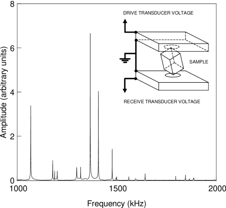
Figure 1: A portion of the resonance spectrum of a rectangular parallelepiped of Sr₂RuO₄ obtained using the RUS technique. The inset shows a schematic of the RUS apparatus.

The resonance frequencies of the Sr₂RuO₄ sample were determined at room temperature using the apparatus shown schematically in the inset of Fig. 1. By holding the sample between two piezoelectric transducers, where one transducer is used to drive the sample with mechanical vibrations and the other to detect the mechanical response of the sample, a frequency sweep allowed a rapid measurement of the resonance modes. It should be noted that the only assumption made in the RUS technique lies in the ability to observe the natural resonances of a solid body under free boundary conditions, allowing a proper comparison between measurement and calculation. The rectangular parallelepiped sample was held only lightly by its corners to minimize suppression of any resonance modes, thus making the free boundary approximation appropriate.

Measurements up to $\sim 3$ MHz provided more than sixty measured resonance frequencies. The central portion of this frequency spectrum is shown in Fig. 1. The first thirty measured frequencies are listed in Table 1 along with those calculated analytically using a program developed specifically for the rectangular parallelepiped sample geometry.Migliori Note that all of the first thirty calculated resonance frequencies were detected, and only three of the next thirty were undetectable. The error is listed as the percentage difference between measured and calculated values. It should be noted that in RUS measurements it is commonly found that the first one or two modes typically have a much larger discrepancy between measured and calculated values than the average, as is seen for the first mode in Table 1, and are therefore not weighted in the fit. The dependence of each mode on the elastic constants was also estimated using this program in order to indicate the pure (shear/compressional) or composite nature of each resonance mode, and are listed as the normalized values $df/dC_{ij}$ in Table 1. For example, the $n=5$ resonance mode can be seen to depend mainly on the constant $C_{66}$, and is thus primarily a pure shear mode. Identification of pure resonance modes can be of use in tracking the behavior of individual elastic constants as a function of temperature or magnetic field.

Table 1: Comparison between measured and calculated values of the first 30 resonance frequencies of the Sr₂RuO₄ sample. Included are the normalized $df/dC_{ij}$ values, which indicate the nature of each resonance mode $n$.

$n$	$f_{meas}$ (MHz)	$f_{calc}$ (MHz)	| error % |	$df/dC_{11}$	$df/dC_{33}$	$df/dC_{23}$	$df/dC_{12}$	$df/dC_{44}$	$df/dC_{66}$
1	0.379947	0.373526	1.69	0.01	0.00	0.00	0.00	0.21	0.78
2	0.461821	0.461405	0.09	1.32	0.03	-0.07	-0.43	0.15	0.00
3	0.698196	0.697239	0.14	1.09	0.04	-0.08	-0.32	0.00	0.27
4	0.761808	0.760115	0.22	0.34	0.01	-0.02	-0.11	0.30	0.48
5	0.855415	0.853657	0.21	0.10	0.01	-0.01	-0.02	0.00	0.93
6	0.868241	0.868475	0.03	0.92	0.07	-0.13	-0.11	0.25	0.01
7	0.902003	0.902758	0.08	1.70	0.02	-0.04	-0.68	0.00	0.00
8	0.907763	0.908625	0.09	1.06	0.01	-0.01	-0.44	0.29	0.10
9	1.069506	1.068929	0.05	0.53	0.06	-0.12	0.04	0.42	0.07
10	1.179531	1.179844	0.03	0.57	0.01	-0.02	-0.21	0.43	0.21
11	1.187974	1.186127	0.16	1.12	0.05	-0.08	-0.35	0.00	0.27
12	1.200415	1.198150	0.19	1.43	0.06	-0.11	-0.44	0.00	0.06
13	1.299958	1.301070	0.09	0.42	0.02	-0.04	-0.09	0.39	0.29
14	1.318483	1.317963	0.04	0.60	0.02	-0.03	-0.22	0.00	0.63
15	1.366880	1.366446	0.03	1.50	0.01	-0.02	-0.64	0.00	0.15
16	1.408010	1.408700	0.05	0.48	0.03	-0.05	-0.12	0.00	0.67
17	1.477300	1.480136	0.19	1.12	0.15	-0.25	-0.05	0.00	0.03
18	1.498835	1.496335	0.17	0.62	0.01	-0.02	-0.23	0.58	0.04
19	1.561982	1.561620	0.02	0.56	0.03	-0.06	-0.10	0.55	0.02
20	1.596411	1.592585	0.24	0.38	0.02	-0.03	-0.08	0.66	0.05
21	1.643878	1.639129	0.29	0.36	0.03	-0.06	-0.02	0.64	0.06
22	1.697681	1.702562	0.29	0.26	0.02	-0.03	-0.04	0.47	0.31
23	1.796324	1.797892	0.09	1.05	0.07	-0.10	-0.31	0.00	0.29
24	1.845635	1.846354	0.04	0.65	0.03	-0.04	-0.23	0.00	0.59
25	1.864200	1.862988	0.07	0.66	0.04	-0.06	-0.20	0.00	0.56
26	1.885902	1.887157	0.07	1.53	0.02	-0.03	-0.65	0.00	0.13
27	1.887384	1.889048	0.09	0.29	0.02	-0.04	-0.01	0.62	0.13
28	1.908689	1.900802	0.41	0.23	0.01	-0.01	-0.07	0.83	0.01
29	1.945637	1.942492	0.16	0.21	0.01	-0.03	-0.03	0.71	0.12
30	1.992652	1.995493	0.14	0.43	0.02	-0.04	-0.11	0.57	0.13

The elastic constants used as initial fitting parameters were estimated using a combination of available values for Sr₂RuO₄Matsui67 ; Lupien and the isostructural material La₂CuO₄Sarrao , and subsequently adjusted through numerous fitting iterations to obtain the best fit. The quality of each fit was calculated using the root-mean-square error $\sigma_{RMS}$ between measured and calculated resonant frequencies,

$$\sigma_{RMS}=100\times\sqrt{\frac{1}{N}\sum_{n=1}^{N}\bigg{(}\frac{f_{meas}^{(n)}-f_{calc}^{(n)}}{f_{calc}^{(n)}}\bigg{)}^{2}}~{}~{}\%,$$ (1)

where $n$ is the mode number and $N$ is the total number of modes weighted in the fit. The fitting procedure resulted in a $\sigma_{RMS}$ value of $0.19\%$ between the measured and calculated frequencies: such a small value is an indication of an excellent fit.Migliori The fitted dimensions agreed with the measured values to within error, also confirming the validity of the fit. The elastic constants calculated using this fit are compared in Table 2 with values obtained for Sr₂RuO₄ from various pulse-echo experiments and with those obtained for La₂CuO₄ using the RUS technique. The absolute accuracy of the constants obtained in this study was based on either a quality-of-fit estimate, obtained from a measure of the stability of the minimization calculation used in the fitting routine, or on errors in density measurement, taking the larger of the two as the conservative approximation. Specifically, the errors on $C_{11}$, $C_{33}$, $C_{23}$, and $C_{12}$ were obtained from quality-of-fit estimates, and those on $C_{44}$ and $C_{66}$ were based on the variation in calculated $C_{ij}$ values obtained from fits using upper and lower dimensional bounds as input parameters.error

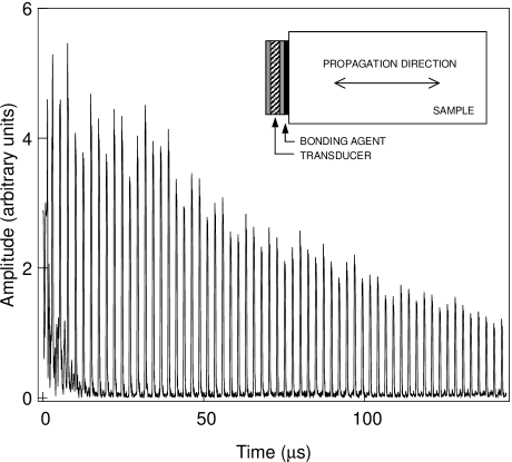
Figure 2: Echo pattern for a transverse sound mode corresponding to $C_{66}$, with propagation in the [100] crystal axis direction and polarization in the [010] direction of Sr₂RuO₄, obtained using the pulse-echo technique on a sample of length 3.98 mm (from Ref. Lupien, ). The inset shows a schematic of a typical pulse-echo setup.

Table 2: Single crystal elastic constants of Sr₂RuO₄. Units are in $10^{12}~{}$dynes/cm².

Source	$C_{11}$	$C_{33}$	$C_{23}$	$C_{12}$	$C_{44}$	$C_{66}$	$(C_{11}-C_{12})/2$	Temperature (K)
this work	$2.32(2)$	$2.08(2)$	$0.71(2)$	$1.06(2)$	$0.657(4)$	$0.612(4)$	$0.63(1)$	$300$
Ref. Lupien,	$2.35(7)$			$1.28(4)$	$0.68(2)$	$0.65(2)$	$0.52(2)$	$<4$
Ref. Lupien,	$2.21(7)$	$2.4(2)$		$1.16(4)$	$0.66(2)$	$0.63(2)$	$0.57(2)$	$300$
Ref. Matsui67,	$\sim 1$	$\sim 0.9$			$\sim 0.1$	$\sim 0.1$		$4.2$
Ref. Matsui69,					$0.4$	$0.38$	$0.37$	$250$
Ref. Okuda,	$1.074$	$0.783$	$0.169$	$0.452$			$0.311$	$4.2$
Ref. Sarrao,  (La2CuO4)	$2.45$	$2.48$	$0.95$	$0.61$	$0.63$	$0.52$	$0.92$	$580$

The elastic constants reported by Lupien et al. were measured at low temperature ($<4$ K) using the pulse-echo technique on samples cut from the same ingot used in this study.Lupien A typical pulse-echo experimental apparatus is shown schematically in the inset of Fig. 2. With this technique, sound velocities are calculated using the length between two parallel faces of an oriented crystal and the measured time delay between echoes of the initial pulse, such as those shown in Fig. 2. By solving the usual Christoffel equations, the elastic constants are obtained from sound velocities measured for various propagation and polarization directions and the mass density.Truell For example, the shear elastic constant,

$$C_{66}=\rho v_{[100/010]}^{2},$$ (2)

is calculated from the mass density $\rho$ and sound velocity $v_{[100/010]}$ (propagating in the [100] direction and polarized in the [010] direction). All of values from Ref. Lupien, shown in Table 2, except for $C_{12}$, are proportional to the square of various velocities directly measured in different propagation and polarization directions (the value for $C_{12}$ is given as an average of two values calculated using two different sound velocities and the value of $C_{11}$). By extrapolating these low-temperature values to 300 K using temperature dependencies found elsewhere,Matsui69 agreement is found to within experimental error for $C_{44}$ and $C_{66}$, and to within $10\%$ for $C_{11}$, $C_{12}$ and $C_{33}$ when compared to the values in this study. The various elastic constants reported by Matsui et al. (Ref. Matsui67, , Matsui69, ) and Okuda et al. (Ref. Okuda, ) are a factor of $\sim 2$ less than these values, which is much greater than the $\sim 6\%$ change in the constants observed from low to room temperature.

The Debye temperature $\theta_{D}$ is estimated from the elastic constants by using the following expression for a tetragonal crystal,Alers

$$\theta_{D}=\frac{h}{k_{B}}\left(\frac{9N}{4\pi V}\right)^{-1/3}\rho^{-1/2}J^{-1/2},$$ (3)

where $h$ and $k_{B}$ are Planck’s and Boltzmann’s constants, respectively, $N/V$ is the atomic density, and $J$ is the series expansion of an integration over sound velocities in all crystal directions, written in terms of the elastic constants (see Eq. 32 in Ref. Alers, ). Using Eq. 3, the full set of elastic constants measured in this study gives $\theta_{D}=465(5)$ K (this value increases by $\sim 5$ K when using values extrapolated to low temperature in a manner similar to that used in Table 2 for Ref. Lupien, ). This elastic measure of $\theta_{D}$ compares well with the value of $410(50)$ K extracted from the $T^{3}$ phonon contribution to specific heat,thetaC and the value of 427(50) K obtained in Mössbauer measurements,thetaM where $\theta_{D}$ is extracted from the temperature dependence of the Debye-Waller factor.

In conclusion, the complete set of elastic constants was obtained for the tetragonal crystal Sr₂RuO₄ using the measured resonance frequencies of a small rectagular parallelepiped sample. Excellent agreement was found with values obtained from pulse-echo experiments performed on a sample cut from the same ingot. The Debye temperature determined from the measured constants was found to compare well with values obtained from other measurements.

This work was supported by the Canadian Institute for Advanced Research and funded by NSERC.  J.P. and C.L. acknowledge the support of the Walter C. Sumner Foundation, and C.L. also acknowledges the support of FCAR (Québec).

References

- (1) Y. Maeno, H. Hashimoto, K. Yoshida, S. Nishizaki, T. Fujita, J. G. Bednorz and F. Lichtenberg, Nature (London) 372, 532 (1994).
- (2) Y. Maeno, T. M. Rice and M. Sigrist, Phys. Today 54, 42 (2001).
- (3) R. Truell, C. Elbaum and B.B. Chick, Ultrasonic Methods in Solid State Physics (Academic Press, New York, 1969), pp. 1-52.
- (4) Z. Q. Mao et al., Mater. Res. Bull. 35, 1813 (2000).
- (5) This value is obtained by calculating the density at 2 K using lattice constants measured via neutron powder diffraction Gardner , and adjusting to room temperature for thermal expansion.Chmaissem
- (6) J. S. Gardner, G. Balakrishnan, D. McK. Paul and C. Haworth, Physica C 265, 251 (1996).
- (7) O. Chmaissem, J. D. Jorgensen, H. Shaked, S. Ikeda and Y. Maeno, Phys. Rev. B 57, 5067 (1998).
- (8) A. Migliori and J.L. Sarrao, Resonant Ultrasound Spectroscopy (Wiley, New York, 1997) and references therein.
- (9) J. Paglione, M.Sc. Thesis (University of Toronto, 2000).
- (10) A. De Visser, A. Menovsky and J.J.M. Franse, Physica B 147, 81 (1987).
- (11) H. Matsui, M. Yamaguchi, Y. Yoshida, A. Mukai, R. Settai, Y. Ōnuki, H. Takei and N. Toyota, J. Phys. Soc. Jpn. 67, 3687 (1998).
- (12) J.L. Sarrao, D. Mandrus, A. Migliori, Z. Fisk, I. Tanaka, H. Kojima, P.C. Canfield and P.D. Kodali, Phys. Rev. B 50, 13 125 (1994).
- (13) The errors chosen according to dimensional bounds were obtained by uniformly increasing (decreasing) the three dimension input parameters in order to use the lower (upper) limit of the measured density in the fitting routine. It should be noted that any non-uniform change in the input dimensions, or in other words the shape of the sample, resulted in a fit with an extremely large RMS error between calculated and measured resonance frequencies, indicating the correct measurement of sample geometry.
- (14) C. Lupien, W.A. MacFarlane, C. Proust, L. Taillefer, Z.Q. Mao and Y. Maeno, Phys. Rev. Lett. 86, 5986 (2001); C. Lupien, Ph.D. Thesis (University of Toronto, 2002).
- (15) H. Matsui, Y. Yoshida, A. Mukai, R. Settai, Y. Ōnuki, H. Takei, N. Kimura, H. Aoki and N. Toyota, J. Phys. Soc. Jpn. 69, 3769 (2000).
- (16) N. Okuda, T. Suzuki, Z. Mao, Y. Maeno and T. Fujita, preprint submitted to SCES’2001 (2001).
- (17) G.A. Alers in Physical Acoustics Vol. IIIB, edited by W.P. Mason (Van Nostrand, Princeton, 1958).
- (18) S. Nishizaki, Y. Maeno, S. Farner, S. Ikeda and T. Fujita, J. Phys. Soc. Jpn. 67, 560 (1998).
- (19) M. De Marco et al., Phys. Rev. B 60, 7570 (1999).