Thermal diffusion of supersonic solitons in an anharmonic chain of atoms

Abstract

We study the non-equilibrium diffusion dynamics of supersonic lattice solitons in a classical chain of atoms with nearest-neighbor interactions coupled to a heat bath. As a specific example we choose an interaction with cubic anharmonicity. The coupling between the system and a thermal bath with a given temperature is made by adding noise, delta-correlated in time and space, and damping to the set of discrete equations of motion. Working in the continuum limit and changing to the sound velocity frame we derive a Korteweg-de Vries equation with noise and damping. We apply a collective coordinate approach which yields two stochastic ODEs which are solved approximately by a perturbation analysis. This finally yields analytical expressions for the variances of the soliton position and velocity. We perform Langevin dynamics simulations for the original discrete system which confirm the predictions of our analytical calculations, namely noise-induced superdiffusive behavior which scales with the temperature and depends strongly on the initial soliton velocity. A normal diffusion behavior is observed for solitons with very low energy where the noise-induced phonons also make a significant contribution to the soliton diffusion.

I Introduction

Nonlinear one-dimensional lattice dynamics, namely propagation of coherent excitations in monatomic chains modeling discrete microscopic structures, is associated with several important problems in physics. Among these excitations are solitary waves, which for simplicity are called here solitons. These solitons can be supported by chains with realistic interaction potentials between the particles Lomdahl ; Lawrence . They are supersonic non-topological collective excitations. In spite of their relative simplicity, the solitons clarify many features of molecular chains Toda ; Pnevmatikos ; Davydov ; Collins ; Hochstrasser1 . For example, due to their robust character, lattice solitons have been used to model the energy transport in polypeptide chains in muscle proteins Yomosa ; Perez ; Perez1 or the energy transport in DNA Muto . Numerical simulations at realistic temperatures for transport in proteins have shown that lattice solitons can propagate over long distances in a chain with the Lennard-Jones potential Perez . Moreover, the lattice solitons are more stable than Davydov solitons if collisions between the two types of solitons are considered Perez1 . There is no clear evidence that lattice solitons like a Toda type, which are non-topological, can exist in thermal equilibrium. This holds both for static properties, like the specific heat, and for dynamics quantities, like the dynamic form factor (Fourier Transform of the displacement autocorrelation) Neuper . On the other hand, there exists evidence from real experiments that strain solitons can be generated and observed in non-linear elastic rods samsonov . These solitons in some cases can be described by Korteweg-de Vries (KdV) type solitons, which are non-topological.

To our knowledge there are no previous analytical studies supported by Langevin simulations about non-topological lattice soliton diffusion in anharmonic monatomic chains of particles with nearest-neighbor interactions. There are many studies on stochastic partial differential equations, in particular stochastic KdV-type equations have been extensively studied numerically and analytically KonotopVazquez ; Wadati ; Wadati2 ; Herman ; Iizuka ; ScalerandiRomano due to the integrability of the KdV equation. In fact, the KdV equation is a good approximation to describe analytically the dynamics of lattice solitons on a monatomic chain with nearest-neighbor interaction and cubic anharmonicity if the soliton velocity is very close to the sound velocity (very-low-energy solitons) Pnevmatikos ; Remoissenet . Notice that for a polynomial potential, namely harmonic term plus cubic or/and quartic anharmonicity, the one-soliton solution of the KdV equation is known analytically, while for more realistic interaction potentials like Lennard-Jones or Morse there are no exact soliton solutions. In the more general context of lattice systems, there are a few analytical studies about diffusion of coherent lattice excitations, viz. stochastic vortex dynamics in two-dimensional easy-plane ferromagnets kampetter or soliton diffusion on the classical, isotropic Heisenberg chain mathias1 ; mathias .

The aim of this work is to provide an approximate analytical description of the soliton diffusion dynamics in a monatomic chain with a cubic anharmonicity under thermal fluctuations. For this purpose we generate a single soliton which has an energy far greater than $k_{B}\,T$, where $k_{B}$ is the Boltzmann constant, and $T$ is the temperature of a thermal bath. This soliton propagating on a chain in contact with the thermal bath shows a diffusive behavior. We consider this soliton diffusion dynamics during the thermalization process of the system up to times when the system energy has relaxed nearly to its stationary value. This means that we study the non-equilibrium diffusion dynamics of lattice solitons on anharmonic chains subject to thermal fluctuations.

In order to perform the coupling between the system and a thermal bath with a given temperature an additive noise term, providing energy input, is added to the discrete equations of motion. This term has to be balanced by a damping term providing energy dissipation. Here, we suggest as a damping term the so-called hydrodynamical damping Landau which is extensively used in, e.g., elasticity theory. Notice that this type of damping is due to irreversible processes taking place within the system. The corresponding noise term, which fulfills the fluctuation-dissipation theorem, takes the form of a discrete gradient of Gaussian white noise delta-correlated in space and time. A similar Langevin-type equations has previously been considered in the context of mesoscopic Langevin dynamics Schmittmann .

We notice that our system in the continuum limit can be approximated by a noisy KdV-Burgers-type equation nozaki ; Orlowski . So in this case we can use the one-soliton solution of the KdV equation not only as initial condition of our discrete system but also in our analytical approach in the continuum limit. Notice that the shape of broad KdV solitons tends to be identical to the shape of broad supersonic lattice solitons Pnevmatikos . In this work we apply a generalized traveling wave ansatz combined with a collective coordinate formalism in the framework of the KdV equation as an analytical approach to study the diffusion of lattice solitons.

In the next section we present the equations of motion of our discrete system. From this we formulate a set of stochastic equations of motion by adding noise and damping. Next, we apply the continuum limit and derive a form of noisy KdV-Burgers equation. In section III we apply a collective coordinate approach which yields analytical expressions for the thermal averages and variances of the soliton position and velocity. In section IV, we compare our analytical predictions with the results from Langevin dynamics simulations for the original discrete system. Our conclusions are summarized in the last section.

II The continuum limit

We consider an anharmonic chain of particles with mass $M$ and nearest-neighbor interactions. The particles interact via an anharmonic potential with a cubic anharmonicity. The Hamiltonian of this system reads

$$H=\sum_{n}\left\{\frac{P_{n}^{2}}{2M}+\right.$$

$$\left.G\left(\frac{1}{2}(Y_{n+1}-Y_{n})^{2}+\frac{A}{3}(Y_{n+1}-Y_{n})^{3}\right)\right\},\quad$$ (1)

where $Y_{n}$ denotes the longitudinal displacement of the $n$-th particle from its equilibrium position, and

$$P_{n}=M\frac{dY_{n}}{dt}$$ (2)

is the momentum. Here $G$ and $A$ are the potential parameters whose values depend on the lattice. The associated first order equations of motion read

$$\frac{dY_{n}}{dt} = \frac{1}{M}P_{n}$$ (3)

$$\frac{dP_{n}}{dt} = -\frac{\partial H}{\partial Y_{n}}+F_{n}^{Noise}+F_{n}^{Damping},$$ (4)

where

$$\frac{\partial H}{\partial Y_{n}} = -G\left(Y_{n+1}-2Y_{n}+Y_{n-1}\right)$$ (5)

$$-GA\left((Y_{n+1}-Y_{n})^{2}-(Y_{n}-Y_{n-1})^{2}\right).\quad\quad$$

In Eq. (4) we have already added both a stochastic force, $F_{n}^{Noise}$, and a damping force,$F_{n}^{Damping}$. Both forces couple the discrete system with a thermal bath. Here, we use the inner or hydrodynamical damping, which reads Landau ; arevalo

$$F_{n}^{Damping}=M\nu\left(\frac{dY_{n+1}}{dt}-2\frac{dY_{n}}{dt}+\frac{dY_{n-1}}{dt}\right).$$ (6)

This means that the energy dissipation is provided by the irreversible processes arising from the finite velocity of the internal motions of the system, namely time derivative of the relative displacements between particles in the chain. Eq. (6) is the discrete version of the damping used in elasticity theory Landau . To fulfill the fluctuation-dissipation theorem the noise must have the form (see App. A)

$$F_{n}^{Noise}=\sqrt{\rm D}\left(\xi_{n+1}(t)-\xi_{n}(t)\right)$$ (7)

where

$${\rm D}=2M\nu k_{B}T$$ (8)

is the diffusion constant and $\nu$ is the damping constant. $\xi_{n}(t)$ is delta-correlated white noise,

$$\left\langle\xi_{n}(t)\xi_{m}(t^{{}^{\prime}})\right\rangle = \delta_{nm}\delta(t-t^{{}^{\prime}}),$$ (9)

$$\left\langle\xi_{n}(t)\right\rangle = 0.$$ (10)

Since our interest is the study of the lattice soliton diffusion close to the sound velocity, $c$, we can use the continuum limit approach, where $Y_{n}(t)\rightarrow y(x,t)$ and $\xi_{n}(t)\rightarrow\xi(x,t)$ with $x=n\,a$ and $a$ the equilibrium atomic spacing. In this limit Pnevmatikos , Eq. (3) reduces to a form of noisy and damped KdV equation (see App. B for details)

$$\partial_{\tau}u+6u\partial_{s}u+\partial_{s}^{3}u=\nu_{1}\partial_{ss}u-\sqrt{D_{1}}\partial_{s}\overline{\xi}(s,\tau)$$ (11)

where

$$s=\alpha(x-ct),\quad\quad\quad\tau=\beta t,\quad\quad\quad u=\gamma\partial_{s}y.$$ (12)

The constants $\alpha$, $\beta$ and $\gamma$ are defined in (87), and $\nu_{1}$ and $D_{1}$ are given by Eqs. (91). Note that

$$\left\langle\overline{\xi}(s,\tau)\overline{\xi}(s^{\prime},\tau^{\prime})\right\rangle=\delta(s-s^{\prime})\delta(\tau-\tau^{\prime}).$$ (13)

Here and in the following the line over $\overline{\xi}$ is omitted.

The case $D_{1}=0$ reduces Eq. (11) to the KdV-Burgers equation. The associated KdV equation is

$$\partial_{\tau}u+6u\partial_{s}u+\partial_{s}^{3}u=0$$ (14)

whose one-soliton solution reads

$$u_{0}(s,\tau)=2\eta^{2}_{0}\,\mbox{sech}^{2}[\eta_{0}(s-4\eta^{2}_{0}\tau-s_{0})].$$ (15)

Here

$$\eta_{0}=\frac{1}{p}\sqrt{3c(v-c)}$$ (16)

is the inverse soliton width and $s_{0}$ is the initial soliton position. The sound velocity $c$ and the constant $p$ are defined in (B.1).

III Collective coordinate approach

To analyze our problem we assume that the soliton profile, $u_{0}(s,\tau)$, is not disturbed by the noise and damping terms and that only the width and amplitude are modified. This assumption is well satisfied for low-energy solitons, whose velocity is close to the sound velocity, because tails induced by the perturbations are small in this velocity regime grim ; arevalo . So we introduce a generalized traveling wave ansatz of the form

$$u(s,\tau) = u_{0}(s-S(\tau),\eta(\tau))$$ (17)

$$= 2\eta^{2}(\tau)\,\mbox{sech}^{2}[\eta(\tau)(s-S(\tau))],$$

where the collective variables $S(\tau)$ and $\eta(\tau)$ are the soliton position and the inverse soliton width, respectively. Here and in the following the index of the one-soliton solution $u_{0}$ is omitted.

To obtain the equations for our collective coordinates we follow niurkaPRE ; Mertens1 . First, by substituting (17) into Eq. (11) we get

$$\phi_{1}\,{\dot{S}(\tau)}+\phi_{2}\,{\dot{\eta}(\tau)}=\nu_{1}\partial_{ss}u-\sqrt{D_{1}}\partial_{s}\xi(s,\tau),$$ (18)

where

$$\phi_{1}(s,\tau)=\frac{\partial u}{\partial S}$$ (19)

and

$$\phi_{2}(s,\tau)=\frac{\partial u}{\partial\eta}.$$ (20)

Notice that the functions $\left\{\phi_{i}\right\}_{i=1,2}$ coincide with the adiabatic approximation (omitting secular terms in time) of the discrete solutions of the linearized KdV equation around the one-soliton solution (15) Mann . We remark here that our collective coordinate theory does not take into account the contribution of the phonon modes (continuous basis function solution of the linearized KdV). We discuss the effect of noise-induced phonons in section IV.2. The functions $\left\{\phi_{i}\right\}_{i=1,2}$ are also orthogonal, so the inner product $\int ds\,\phi_{i}(s,\tau)\,h(s,\tau)$ projects a function $h$ onto the functions $\left\{\phi_{i}\right\}_{i=1,2}$. Then, by projecting Eq. (18) we get

$$A_{i}{\dot{S}}(\tau)+B_{i}{\dot{\eta}}(\tau)=f_{i}+f_{i}^{damping}+f_{i}^{Noise}\quad\quad i=1,2\quad,$$ (21)

where

$$A_{i} = \int ds\frac{\partial u}{\partial S}\,\phi_{i},$$ (22)

$$B_{i} = \int ds\frac{\partial u}{\partial\eta}\,\phi_{i},$$ (23)

$$f_{i} = \int ds\left(6u\partial_{s}u+\partial_{s}^{3}u\right)\phi_{i},$$ (24)

$$f_{i}^{damping} = \nu_{1}\int ds\partial_{ss}u\,\phi_{i},$$ (25)

$$f_{i}^{Noise} = -\sqrt{D_{1}}\int ds\partial_{s}\xi(s,\tau)\,\phi_{i}.$$ (26)

After some calculations the Eqs. (21) take the form

$$\frac{dS(\tau)}{d\tau}=4\eta^{2}(\tau)+\frac{15\sqrt{D_{1}}}{64\eta^{5}(\tau)}\int ds(\partial_{s}\phi_{1})\xi(s,\tau),\quad\quad$$ (27)

$$\frac{d\eta(\tau)}{d\tau}=-\frac{30\nu_{1}}{30+\pi^{2}}\eta^{3}(\tau)+$$

$$\quad\quad\quad\frac{45\sqrt{D_{1}}}{16(30+\pi^{2})\eta(\tau)}\int ds(\partial_{s}\phi_{2})\xi(s,\tau).$$ (28)

To achieve the calculations we have assumed that the soliton profile remains mostly unaffected and only its width and amplitude change due to the stochastic perturbations. Then, at least for small noise, we can perform the calculations by taking the soliton field out of the averages. Moreover, we have interpreted Eqs. (27) and (III) in the Stratonovich sense, because it assumes $\xi(s,\tau)$ is a real noise with finite correlation time, which is then allowed to become infinitesimally small after calculating measurable quantities Gardiner . Notice that white noise means taking the limit of zero correlation time.

Eqs. (27) and (III) can take the form

$$\frac{d{\bf Y}(\tau)}{d\tau}={\bf A}^{Str}[{\bf Y}(\tau)]+\int ds\hat{\bf B}^{Str}[s,{\bf Y}(\tau)]\mbox{\boldmath$\xi$}(s,\tau),$$ (29)

where the elements of the noise vector $\xi$ satisfy (13). $\{Y_{1},Y_{2}\}=\{S,\eta\}$ are the elements of the vector ${\bf Y}$, the elements $\{A^{Str}_{1},A^{Str}_{2}\}$ of the drift vector ${\bf A}^{Str}$ are the drift terms in Eqs. (27) and (III), respectively. The diffusion matrix $\hat{\bf B}^{Str}$ is diagonal, where $B^{Str}_{11}$ and $B^{Str}_{22}$ are the coefficients in front of the noise in Eqs. (27) and (III), respectively. In order to facilitate the calculations we write Eq. (29) in the Ito form,

$$d{\bf Y}(\tau)={\bf A}^{Ito}[{\bf Y}(\tau)]d\tau+\int ds\hat{\bf B}^{Ito}[s,{\bf Y}(\tau)]d{\bf W}(s,\tau),$$

where the $d{\bf W}(s,\tau)=\mbox{\boldmath$\xi$}(s,\tau)d\tau$ is a Wiener process. Via a Fokker-Planck equation, one can show that the elements of the drift vector ${\bf A}^{Ito}$ read Gardiner

$$A^{Ito}_{i}[{\bf Y}(\tau)]=A^{Str}_{i}[{\bf Y}(\tau)]+$$

$$\quad\quad\quad\frac{1}{2}\sum_{j\,k\,m}\int dsB^{Str}_{k\,m}[s,{\bf Y}(\tau)]\partial_{Y_{k}}B^{Str}_{i\,j}[s,{\bf Y}(\tau)]$$

$$\quad\quad\quad i,j,k=1,2$$ (31)

while

$$\hat{\bf B}^{Ito}[s,{\bf Y}(\tau)]=\hat{\bf B}^{Str}[s,{\bf Y}(\tau)].$$ (32)

Notice that ${\bf A}^{Ito}$ and $\hat{\bf B}^{Ito}$ are nonanticipating functions. So, from Eq.(III) it is easy to show the following averages

$$\left\langle S(\tau)\right\rangle = \langle\int\limits_{0}^{\tau}d\tau^{\prime}4\eta^{2}(\tau^{\prime})\rangle$$

$$\left\langle\eta(\tau)\right\rangle = -\bigg{\langle}\int\limits_{0}^{\tau}d\tau^{\prime}\frac{30\nu_{1}}{30+\pi^{2}}\eta^{3}(\tau^{\prime})\bigg{\rangle}+$$

$$\int\limits_{0}^{\tau}d\tau^{\prime}\frac{225(231+8\pi^{2})D_{1}}{112(30+\pi^{2})^{2}}$$

$$Var\left(S(\tau)\right) = \bigg{\langle}\int\limits_{0}^{\tau}d\tau^{\prime}\frac{75\,D_{1}}{112\,\eta^{3}(\tau^{\prime})}\bigg{\rangle}$$

$$Var\left(\eta(\tau)\right) = \bigg{\langle}\int\limits_{0}^{\tau}d\tau^{\prime}\frac{225(21+\pi^{2})\,D_{1}\eta(\tau^{\prime})}{28(30+\pi^{2})^{2}}\bigg{\rangle}$$

$$Corr\left(S(\tau)\eta(\tau)\right) = 0.$$ (33)

Here $\langle\,\cdot\cdot\cdot\,\rangle$ means average over an ensemble of realizations,

$$Corr(PQ)=\langle\,PQ\,\rangle-\langle\,P\,\rangle\langle\,Q\,\rangle\quad\textrm{and}\quad Var(P)=Corr(PP).$$ (34)

Now we define a new set of Langevin equations,

$$dY_{i}(\tau)=a_{i}d\tau+\sum_{j}b_{ij}\,dW_{j}(\tau)$$

$$\textrm{with}\quad i,j=1,2\quad\textrm{and}\quad\{Y_{1},Y_{2}\}=\{S,\eta\},$$ (35)

which we have interpreted in the Ito sense. $dW_{j}(\tau)=\xi_{j}(\tau)d\tau$ are Wiener processes where we have let the noises to be uncorrelated, namely

$$\langle\xi_{j}(\tau)\xi_{j^{\prime}}(\tau^{\prime})\rangle=\delta(\tau-\tau^{\prime})\delta_{jj^{\prime}}.$$ (36)

In order to determine the values of $a_{i}$ and $b_{ij}$ we have demanded that Eqs.(III) satisfy the relations (III). It is straightforward to see that Eqs. (III) take the form

$$dS(\tau) = 4\eta^{2}(\tau)d\tau+\frac{5\sqrt{3}}{4\sqrt{7}}\sqrt{\frac{D_{1}}{\eta^{3}(\tau)}}\,dW_{1}(\tau)$$ (37)

$$d\eta(\tau) = \bigg{(}-\frac{30\nu_{1}}{30+\pi^{2}}\eta^{3}(\tau)+\frac{225(231+8\pi^{2})D_{1}}{112(30+\pi^{2})^{2}}\bigg{)}d\tau+$$ (38)

$$\frac{15\sqrt{21+\pi^{2}}}{2\sqrt{7}(30+\pi^{2})}\sqrt{D_{1}\eta(\tau)}\,dW_{2}(\tau).$$

Eqs. (37) and (38) are statistically equivalent to Eqs (27) and (III) because they share the same Fokker-Planck equation. Since the derivation of Eqs (37) and (38) involved approximations, we have not solved them exactly. Instead of that, we have used perturbation analysis Abdullaev , which is developed in detail in App. C. In order to do so, we have considered the thermal terms as perturbations, so Eqs. (37) and (38) take the form

$$dS(\tau) = 4\eta^{2}(\tau)d\tau+\epsilon\frac{5\sqrt{3}}{4\sqrt{7}}\sqrt{\frac{D_{1}}{\eta^{3}(\tau)}}\,dW_{1}(\tau)$$ (39)

$$d\eta(\tau) = -\frac{30\nu_{1}}{30+\pi^{2}}\eta^{3}(\tau)d\tau+\epsilon\bigg{(}\frac{225(231+8\pi^{2})D_{1}}{112(30+\pi^{2})^{2}}d\tau+$$ (40)

$$\frac{15\sqrt{21+\pi^{2}}}{2\sqrt{7}(30+\pi^{2})}\sqrt{D_{1}\eta(\tau)}\,dW_{2}(\tau)\bigg{)}.$$

Now, we seek an asymptotic solution in the form of a small-noise expansion

$$S(\tau)=s_{0}(\tau)+\epsilon\,s_{1}(\tau)+\cdot\cdot\cdot$$

$$\eta(\tau)=\eta_{0}(\tau)+\epsilon\,\eta_{1}(\tau)+\cdot\cdot\cdot.$$ (41)

Here, $\epsilon$ is a factor introduced for convenience in the analytical calculations. Notice that the case $\epsilon=0$ reduces Eqs. (39) and (40) to the deterministic case. In order to interpret our perturbation theory we must set $\epsilon=1$ and assume that the terms on the r.h.s. of Eqs. (39) and (40) are sufficiently small. So we must restrict ourselves to a regime of low temperatures of the thermal bath ($D_{1}$ small). From the perturbation analysis we obtain that

$$\langle S(\tau)\rangle = \langle s_{0}(\tau)\rangle+\langle s_{1}(\tau)\rangle$$

$$= 4\frac{\eta_{0}^{2}(0)}{\lambda}\log{(1+\lambda\tau)}+\frac{15D_{1}\,(231+8\pi^{2})\,\eta_{0}(0)\,(2(1+\lambda\tau)^{5/2}-5\lambda\tau-2)}{7(30+\pi^{2})^{2}\lambda^{2}(1+\lambda\tau)},$$

$$\langle 4\,\eta^{2}(\tau)\rangle = \langle 4\,\eta_{0}^{2}(\tau)+8\eta_{0}(\tau)\eta_{1}(\tau)\rangle$$

$$= \frac{4\,\eta_{0}^{2}(0)}{1+\lambda\tau}+\frac{45D_{1}(231+8\pi^{2})\,\eta_{0}(0)\,((1+\lambda\tau)^{5/2}-1)}{7(30+\pi^{2})^{2}\lambda\,(1+\lambda\tau)^{2}},$$

$$Var(S(\tau)) = D_{1}\bigg{(}\frac{-15}{56\,\eta^{3}_{0}(0)\,\lambda}-\frac{480\,(21+{\pi}^{2})\eta^{3}_{0}(0)(8+7\lambda\tau(5\lambda\tau+4))}{49\,{\left(30+{\pi}^{2}\right)}^{2}\,{\lambda}^{3}\,{\left(1+\lambda\,\tau\right)}^{2}}$$

$$+ \frac{15\,(1+\tau\,\lambda)^{3/2}}{392\,{\left(30+{\pi}^{2}\right)}^{2}\,\eta^{3}_{0}(0)\,{\lambda}^{3}}\left(2048(21+\pi^{2})\eta^{6}_{0}(0)+7(30+\pi^{2})^{2}\lambda^{2}(1+\lambda\tau)\right)\bigg{)},$$

$$Var(4\,\eta^{2}(\tau)) = \frac{7200D_{1}(21+\pi^{2})\eta^{3}_{0}(0)}{49\lambda(30+\pi^{2})^{2}}\bigg{(}\frac{1}{\sqrt{1+\lambda\tau}}-\frac{1}{(1+\lambda\tau)^{4}}\bigg{)}.$$

The expressions for $D_{1}$ and $\lambda$ are given by Eqs. (91) and (101), respectively.

IV Simulations

Substituting Eqs. (6) and (7) into Eq. (3) we get the full set of discrete equations of motion written in absolute displacements. However, for our simulations relative displacements are more convenient, because the lattice solitons in this representation are pulse solitons whose amplitude vanishes at infinity. This characteristic allows us to use periodic boundary conditions which are necessary for long simulation times, because we want to avoid reflections at the boundaries. So the discrete equations of motion in relative displacements read

$$M\frac{d^{2}V_{n}}{dt^{2}}=G\left(V_{n+1}-2V_{n}+V_{n-1}\right)+$$

$$\quad\quad GA\left(V_{n+1}^{2}-2V_{n}^{2}+V_{n-1}^{2}\right)+$$

$$\quad\quad M\nu\left(\frac{dV_{n+1}}{dt}-2\frac{dV_{n}}{dt}+\frac{dV_{n-1}}{dt}\right)+$$

$$\quad\quad\sqrt{\rm D}\left(\xi_{n+1}(t)-2\xi_{n}(t)+\xi_{n-1}(t)\right),$$ (43)

where $V_{n}(t)=Y_{n+1}(t)-Y_{n}(t)$ and ${\rm D}=2M\nu k_{B}T$. The periodic boundary conditions read

$$\frac{d^{l}\,V_{0}}{dt^{l}}=\frac{d^{l}\,V_{N-1}}{dt^{l}}, \frac{d^{l}\,V_{N}}{dt^{l}}=\frac{d^{l}\,V_{1}}{dt^{l}},\quad\quad l=0,1$$

$$\xi_{0}(t)=\xi_{N-1}(t), \xi_{N}(t)=\xi_{1}(t),$$ (44)

where $N$ is the number of particles of our chain and $N-1$ is the number of bonds.

A suitable method to detect the position of a pulse lattice soliton, $V_{n}(t)$, is to search for its maximum arevalo . However, in the presence of stochastic perturbations this method is not useful since the pulse shape is strongly masked by the noise, an example of this situation is shown in App. E. So from the data of our simulations we have taken snapshots of the system at different times, and from them we have generated the kink shape $Y_{n}(t)$ of the lattice soliton by using the algorithm

$$Y_{n}(t)=Y_{1}(t)+\sum_{i=1}^{n-1}V_{i}(t)\quad n=2,3,\cdot\cdot\cdot,N.$$ (45)

The kink shape is less distorted by the noise than the pulse shape $V_{i}(t)$. In (45) $Y_{1}(t)$ is a boundary condition that we have demanded to be

$$Y_{1}(t)=-\frac{1}{2}\sum_{i=1}^{N-1}V_{i}(t),$$ (46)

so at $t=0$ the amplitude of the center of the kink shape is zero, as it should be from the theory Pnevmatikos . Notice that

$$Y_{N}(t)-Y_{1}(t)=\sum_{i=1}^{N-1}V_{i}(t)$$ (47)

is a conserved quantity in our system, i.e.

$${\dot{Y}}_{N}(t)-{\dot{Y}}_{1}(t)=\sum_{i=1}^{N-1}{\dot{V}}_{i}(t)=0.$$ (48)

We have checked Eq. (48) with a precision higher than $10^{-14}$ over the whole time range of our Langevin dynamics simulations.

In order to determine every time the parameters of the soliton, namely soliton velocity $v$ and position $x$, we have proceeded as follows. We have searched for the values of the parameters $x$ and $v$ where the relation

$$\sum\limits_{n=n_{0}-n_{1}}^{n_{0}+n_{1}}\left(Y_{n}-y_{0}(n\,a-x,v)\right)=0$$ (49)

is fulfilled. Here

$$y_{0}(n\,a-x,v)=\frac{6\sqrt{2\,h\,c(v-c)}}{p}\tanh\left(\frac{n\,a-x}{L(v)}\right)$$ (50)

with

$$L(v)\,=\,(\alpha\,\eta(t))^{-1}\,=\,2\sqrt{\frac{h}{2\,c\,(v-c)}}.$$ (51)

Here the function $\eta$ is defined in (16) and the constants $h$, $p$, $c$ and $\alpha$ are defined in (B.1) and (87). the function (50) is the absolute displacement representation of the one-soliton solution (15) in a frame moving with the soliton velocity. In Eq. (49)

$$n_{0}=\textrm{int}(x)\quad\textrm{and}\quad n_{1}=\textrm{int}(\frac{3}{2}L(v(0))),$$ (52)

where $\textrm{int}(\cdot)$ denotes the integer part of a number and $v(0)$ is the initial soliton velocity. The value of $n_{1}$ has been chosen to take into account only the core of the lattice kink-shape and it is constant during our simulations. In order to determine both $x$ and $v$ we consider different values of $v$ in Eq. (49) within a range of velocities around the initial soliton velocity, namely $v-c\,\in\,[0.1\,(v(0)-c),2\,(v(0)-c)]$. For every value of $v$ we search the value $x$ that fulfills Eq. (49), so we get a set of pairs of values $x$ and $v$. Finally, from this set of pairs of values we search, by using linear interpolation, the values of $x$ and $v$ which fulfill the relation

$$\frac{\sum\limits_{n=n_{0}-n_{1}}^{n_{0}+n_{1}}Y_{n}\,y_{0}(n\,a-x,v)}{\sum\limits_{n=n_{0}-n_{1}}^{n_{0}+n_{1}}(y_{0}(n\,a-x,v))^{2}}=1\quad.$$ (53)

Notice that in Eqs. (49) and (53) we have assumed that the lattice kink shape, $Y_{n}$, is closely related with the function $y_{0}$, however, as was mentioned in Ref. arevalo , a pulse lattice soliton in the presence of damping develops a tail. The amplitude of this trailing tail depends on both soliton the velocity and the damping, so it is bigger when the damping and/or the soliton velocity is higher. Thus, we restrict ourselves to velocities very close to the sound velocity where the effect of this trailing tail is negligible.

Up to now we have determined the parameters $x$ and $v$, which fit the function $y_{0}$ to the lattice kink shape $Y_{n}$, so we have not measured directly either $x$ or $v$. Since the function $y_{0}$ is closely related to the lattice kink-shape $Y_{n}$, one could assume both $x$ and $v$ as an estimate of the soliton position and velocity, respectively. However, we have taken only the parameter $v$ as an estimate of the soliton velocity and with this value we have used a different method to determine the soliton position. In fact, in order to be in agreement with our collective coordinate approach, where we have projected the equations of motion onto the Goldstone mode $\phi_{1}$ (Eq. (19)), we have projected the noisy kink shape $Y_{n}(t)$ onto the pulse solution $u_{0}$ defined in (15). Notice that in the absolute displacement representation the function $u_{0}$ is the Goldstone mode. So this projection reads

$$P(x)=\sum_{i=n-n_{2}}^{n+n_{2}}Y_{i}(t)u_{0}(i\,a-x,v)$$ (54)

where

$$u_{0}(i\,a-x,v)=\frac{6c(v-c)}{p}\mbox{sech}^{2}\left(\frac{i\,a-x}{L(v)}\right)$$ (55)

and $x=n\,a$. The value of $n_{2}$ in Eq. (54) is much larger than the soliton width, so the boundary effects are negligible. The function $u_{0}(i\,a-x,v)$ is the one-soliton solution (15) in a frame moving with the soliton velocity. Afterwards we have searched, by linear interpolation, the value $x$ where $P(x)$ vanishes and we have defined it as the position of the soliton center of mass. At this point we remark that the values of $x$ following from this latter method are not significantly different from the values of $x$ following from the former method (Eqs. 49 and 53). However, we consider the latter method to be more appropriate than the former one in the sense that we proceed in our code in a similar way as in our analytical calculations.

Our Langevin dynamics simulations were performed for a chain with 1500 lattice points. The time integration was carried out by using the Heun method Heun , which has been successfully used in the numerical solution of partial differential equations and difference-differential equations, coupled to either an additive or a multiplicative noise term kampetter ; niurka1 ; mathias1 ; mathias . Here, we have used the conserved quantity (47) to check the accuracy of our code arevalo . For the longest simulation time the variation of this conserved quantity has been lower than $10^{-9}\,\%$. In order to start the simulations at $t=0$ we have used the one-soliton solution (15) of the KdV equation in the laboratory frame. The average values have been calculated over 200 realizations up to a final time 5000. All values of the constants of the equation (IV) are set at unity except the damping constant which is set at $\nu=0.003$. Notice that for lower values of damping the relaxation of the system energy would take more time in our simulations to reach a regime close to its stationary value. On the other hand, higher values of damping can strongly distort the soliton shape, namely the tail induced by the damping cannot be neglected when the value of the damping is high. In App. D we show the thermalization process in our system. In our simulations the values of temperature, $T$, and initial soliton velocity, $v(0)$, are parameters (see figure captions).

Figure 1: Averaged soliton position (a) and velocity (b) vs. time in the sound velocity frame $z=x-t$ ($c=1$), with $\nu\,=\,0.003$ and $T=5\times 10^{-5}$. Dotted lines: simulation, solid lines: theory (Eqs.(III)). A, B, C, D, and E correspond to different initial velocities, namely $\,v(0)=1.001$, $1.003$, $1.005$ and $1.007$, respectively.

Figure 2: Variances of the soliton position (panels a, c and e) and velocity (panels b, d and f) of the soliton vs. time, with $\nu\,=\,0.003$ and $T=5\times 10^{-6}$. Dotted lines: simulation, solid lines: theory (Eqs.(C) and (105)). The panels correspond to different initial velocities, namely $\,v(0)=1.003$ (a and b), $1.005$ (c and d) and $1.007$ (e and f). The reduced temperatures are $\overline{T}=0.0061419$, $0.00283324$, $0.00169765$, respectively.

Figure 3: Variances of the soliton position (panels a, c and e) and velocity (panels b, d and f) of the soliton vs. time, with $\nu\,=\,0.003$ and $T=5\times 10^{-5}$. Dotted lines: simulation, solid lines: theory (Eqs.(C) and (105)). The panels correspond to different initial velocities, namely $\,v(0)=1.003$ (a and b), $1.005$ (c and d) and $1.007$ (e and f). The reduced temperatures are $\overline{T}=0.061419$, $0.0283324$, $0.0169765$, respectively.

IV.1 Soliton propagation

In Figs. 1a and 1b we show several examples of both the averaged soliton position, $\langle x(t)\rangle$, and the averaged soliton velocity, $\langle v(t)\rangle$, as functions of time from both the simulation and the theory (see Eqs.(III)). Notice that

$$\langle x(t)\rangle=\frac{1}{\alpha}\langle S(\beta\,t)\rangle+c\,t$$ (56)

and

$$\langle v(t)-c\rangle=\left(\frac{p^{2}}{12\,c}\right)\langle 4\,\eta^{2}(\beta\,t)\rangle.$$ (57)

For all cases the soliton position from the simulation agrees well with the position given by the analytical theory. In the case of the soliton velocity, the agreement is better for initial velocities close to the sound velocity than for higher velocities. In fact, the time evolution of the velocity given by the simulation is always higher than the theoretical prediction. This systematic difference may be due to the small tail that is generated by the lattice soliton since it is a non-topological soliton arevalo . So it may affect our numerical method for determining the soliton position. We point out that the amplitude of this tail depends on both the soliton velocity and the damping constant, and can be neglected only for velocities close to the sound velocity and small values of the damping constant arevalo . This is the most important reason for restricting our study to low-energy solitons whose velocities are close to the sound velocity. Since this difference is systematic it does not play any role in the numerical calculation of the variances which is our more important goal in this article.

IV.2 Soliton diffusion

In Figs. 2 and 3 we show the variances of the soliton position and velocity vs. time for different initial velocities. The temperature of the thermal bath in Fig. 3 is 10 times higher than that in Fig. 2. The results scale very well by a factor of 10; i.e. the variances are proportional to the temperature, as expected from Eqs. (III).

Notice that our theory (solid lines) has no adjustable parameters. Taking into account that the theory consists of several steps (discrete system $\rightarrow$ Bq equation $\rightarrow$ KdV equation $\rightarrow$ collective coordinate theory $\rightarrow$ perturbation analysis) it is already a significant success to obtain the observed results, as seen in Figs. 2 and 3

We observe that the behavior of the variances depends strongly on the initial soliton velocity. For low-energy solitons, whose velocities are close to the sound velocity (Figs. 2 and 3, cases (a) and (b)), the soliton diffusion tends to be nearly normal, i.e. linear in time. In fact, our theory predicts a normal diffusion for times

$$t\,<<t^{*}=\,\left(\frac{30+\pi^{2}}{495}\right)\left(\frac{c}{\nu\,(v(0)-c)}\right).$$ (58)

This estimate was obtained by comparing the first with second terms of the Taylor expansion in powers of $\tau$ of the variance of the velocity (see Eq. (C)). For low-energy solitons ($v(0){}^{>}_{\sim}\,c$) $t^{*}$ is much larger than our simulation time (Figs. 2a and 3a). This means that the superdiffusivity is not very dominant. However, for higher-energy solitons the anomalous behavior turns out to be important after some time. In those cases $t^{*}$ is comparable with our simulation time (Figs. 2e and 3e).

In the case of solitons with very low energy the variance of the position (Figs. 2a and 3a) does not agree so well with the theoretical prediction. In fact, we observe a transient behavior for times $t\,{}^{<}_{\sim}3/\nu=1000$ where the system energy shows a fast relaxation process (see App. D). Those discrepancies between theory and simulations may be due to the combination of two effects. First, the profile of low-energy solitons is strongly masked by the noise, so the numerical detection of the position can be distorted. Second, not only the noise but also the noise-induced phonons can make a significant contribution to the variance of the position, since the reduced temperature, $\overline{T}=k_{B}\,T/H(0)$ (temperature in units of the initial soliton energy $H(0)$), of the thermal bath is higher here than in the other cases (see captions Figs. 2 and 3). In this respect we estimate the phonon effect on the diffusion of low-energy solitons in the next section (see also Fig. 4).

Notice that the variance of the soliton position is larger for low-energy solitons (Figs. 2a and 3a) than for higher-energy solitons (for instance Figs. 2e and 3e). This is due to the fact that the higher-energy solitons are more robust against thermal fluctuations than the lower-energy ones. Or, equivalently, the reduced temperature $\overline{T}$ of the thermal bath is higher for slow solitons than for the fast ones (see captions of Figs. 2 and 3).

On the other hand, the superdiffusive behavior is more pronounced for higher-energy solitons. This is because the soliton velocity turns out to be more sensitive to the thermal fluctuations in this case than in the case of broader solitons. Notice that the soliton velocity and soliton width are related. Also, since the higher-energy solitons encompass few lattice sites, the soliton-width perturbations are larger with respect to the averaged soliton width in this case than in the case of broader solitons (low-energy solitons). In fact, the variance of the soliton velocity shows this effect, namely that for broader solitons (Figs. 2b and 3b) this variance is smaller than for narrower solitons (for instance Figs. 2f and 3f). The discrepancy between our theory and the numerical simulations for higher-energy solitons (Figs. 2 and 3, cases (c)-(f)) is mainly due to the fact that our theory is valid only for soliton velocities close to the sound velocity.

With respect to the variance of the soliton velocity (Figs. 2 and 3, panels b, d and e) we observe that it is mostly anomalous and its behavior is nearly quantitatively predicted by our theory for $0\,\leq\,t\,{}^{<}_{\sim}\,2000$ in all the cases. For larger times, $2000\,\leq\,t\,<\,5000$, there is a discrepancy which becomes larger with increasing initial velocities.

We remark that the numerical results shown in Figs. 2 and 3 do not change for systems with the double number of sites, namely 3000.

We comment that there was a previous attempt by Scalerandi et al. ScalerandiRomano to calculate theoretically the mean square displacement of a KdV soliton subject to stochastic fluctuations. They considered the case of small Stokes damping and a simple white noise delta-correlated in time and space. Though their theoretical result shows the appearance of a noise-induced superdiffusive behavior, it does not have the same dependence with respect to the soliton width as our results (III), which agree well with our simulations.

IV.3 Estimate of the phonon contribution

In order to estimate this contribution we have performed the following numerical test. We have simulated the propagation of low-energy solitons under thermal fluctuations up to a time (e.g. 2500) when the system energy is close to its stationary value (see App. D). Notice that the diffusion of low-energy solitons is mostly normal (see Figs 2a and 3a). Afterwards, we have isolated the system from the thermal bath by switching off noise and damping, so that solitons propagate only in the noise-induced phonon bath. The diffusion is mostly normal before and after the system is isolated, i.e. the variance of the position is linear in time. We have compared the slope of the variance of the isolated system ($t\,>\,2500$) with the slope of the variance in the case when the system is in contact with the thermal bath the whole time. An example of this test is shown in Fig. 4. We observe that both slopes, after switching off noise and damping, are different. In a normal diffusion process the slope of the variance of the soliton position is the diffusion constant. We call this $D_{total}$ when the system is in contact with the thermal bath since there is a contribution of both the thermal fluctuations and the phonons. The diffusion constant due to the noise-induced phonon bath (isolated system) is termed $D_{ph}$. On the other hand, our theoretical diffusion constant, $D_{th}$, is defined as the linear coefficient of the Taylor expansion of $Var(x(t))$ (see Eqs. (C) and (105)). Since our theory does not take into account the contribution of phonon modes, we expect that the value $D_{noise}=D_{total}-D_{ph}$ may be of the same order of magnitude of $D_{th}$. We observe in Fig. 5 that the relative deviation of $D_{th}$ from $D_{noise}$, $((D_{noise}-D_{th})/D_{noise}$, has the same order of magnitude of $D_{th}$ which is not surprising since the soliton shape is strongly masked and distorted by the noise (see App. E). In this respect we remark that from our results in Figs. 2 and 3 we observe that

$$\sqrt{Var(x(t))}\,<\,L(v(t)),$$ (59)

where the soliton width $L(v(t))$ is defined in (51). The relation (59) means that the stochastic deviations of the soliton center from its mean value are relatively small compared with the soliton width. So the diffusive dynamics of the soliton position evolves inside the soliton core. Thus, this dynamics is very sensitive to the fluctuations of the soliton shape. Notice that our method of determining the soliton position depends implicitly on the soliton shape. So in the case of low-energy solitons, where the shape is strongly masked by the noise, the uncertainties of the method of soliton detection are relatively large compared with the diffusive dynamics of the soliton position. This is because the diffusive dynamics is relative small with respect to the soliton width. In this respect we note that higher-energy solitons present a well defined shape, i.e. the thermal fluctuations are small respect to the soliton amplitude, so the variance of the soliton position, given by our detection method, indeed agrees better with our theory. (see 2c and 3c). Finally, we stress that in our tests the phonon contribution to the soliton diffusion could be clearly observed only for very low-energy solitons (Figs. 2 and 3, cases (c) and (e)), for higher-energy solitons the effect is negligible, namely $D_{ph}\simeq 0$.

Figure 4: An example of a test to determine the phonon contribution to the diffusion constant. Comparison of the behavior of $Var(x)$ from simulations (dotted lines) when the system is in contact (A) and isolated (B: noise and damping are switched off for $t>2500$) from the thermal bath. The slope of the straight lines (solid lines) fitted to the simulation data (dotted) in both cases give the observable values of the diffusion constant, namely $D_{total}$ (A) and $D_{ph}$ (B). The difference can be compared with the slope $D_{th}$ of the dashed line (linear part of the theory, Eq. (C)). $v(0)=1.003$, $T=5\times 10^{-6}$, $\overline{T}=0.0061419$.

Figure 5: Relative deviation $((D_{noise}-D_{th})/D_{noise})$ of the diffusion coefficient vs. $k_{B}\,T/H(0)=\overline{T}$ with $v(0)=1.003$.

IV.4 Estimate of the bath temperature in real physical systems

To clarify the physical meaning of the obtained results we have estimated the soliton energy and characteristic temperature of the thermal bath for two systems where solitons are believed to play an essential role: $\alpha$-helical proteins Perez and crystal inertial gases ballistic . In both cases the Lennard-Jones (LJ) interaction potential,

$$\phi_{LJ}=4E_{0}\left(\left(\frac{a}{r}\right)^{12}-\left(\frac{a}{r}\right)^{6}\right),$$ (60)

is used. One can estimate the potential parameters $G$ and $A$ of the Hamiltonian (II) by using Taylor expansion of (60) around the minimum $r=(1-2^{1/6})a$. So, taking into account only the coefficients of the harmonic and cubic terms of this expansion, one can determine the potential parameters, namely

$$A=-\frac{21}{2^{7/6}a}\quad\textrm{and}\quad G=\frac{36\,2^{2/3}\,E_{0}}{a^{2}}.$$ (61)

By using the one-soliton solution of the Bq equation (79) Pnevmatikos and performing an integration instead of a summation in Eq. (II), the initial soliton energy $H(0)$ reads

$$H(0)=\frac{16\sqrt{3}}{245}((v/c)^{2}-1)^{3/2}(1+9(v/c)^{2})E_{0}.$$ (62)

Here $v$ and $c$ are the soliton and sound velocities, respectively. $E_{0}=0.22\,eV$ for $\alpha$-helix Perez or $E_{0}=1.0\times 10^{-2}\,eV$ for argon argon . So, for example, in the cases of $v/c$=1.003 or 1.03 we get

	$\alpha$-helix	argon
$v/c$	$H(0)/k_{B}$ [K]	$H(0)/k_{B}$ [K]
1.003	1.4	0.06
1.03	45.7	2.15

Here $k_{B}$ is the Boltzmann constant. Then, the value of the temperature of the thermal bath can be obtained by multiplying the values of $H(0)/k_{B}$ by the reduced temperature. For instance, in the $\alpha$-helix case the reduced temperature $\overline{T}=0.061419$ (see caption Fig. 3) corresponds to $0.1\,K$ of the thermal bath if $\,v(0)=1.003$ or $3.8\,K$ if $\,v(0)=1.03$.

V Summary and conclusions

We have studied the non-equilibrium diffusion dynamics of lattice solitons on a classical chain of atoms under thermal fluctuations, namely soliton dynamics when the system energy is close to its stationary value. The interaction potential between the atoms is harmonic plus a cubic anharmonicity. The chain is coupled to a thermal bath at a given temperature. For that reason we have included dissipation and noise in the discrete equations of motion of the chain. Here, it is assumed that the energy dissipation is provided by the irreversible processes arising from the finite velocity of the relative displacements between particles in the chain. Thus the dissipative term takes the form of a hydrodynamical damping which is extensively used in elasticity theory. The noise term which fulfills the fluctuation-dissipation theorem then becomes a discrete gradient of white noise delta-correlated in space and time. In the continuum approach our original discrete set of equations leads to a form of noisy KdV-Burgers equation. At this point we have used a collective coordinate approach to study the diffusion dynamics of both position and velocity of the soliton. The soliton position and the inverse soliton width have been found to be good collective coordinates to describe the soliton diffusion. We have derived two stochastic ordinary differential equations with multiplicative noise which have been solved analytically using stochastic perturbation analysis.

For low-energy solitons, whose velocities are close to the sound velocity, our molecular dynamics simulation has confirmed our analytical predictions. Namely, normal diffusion of lattice solitons governs short times, while superdiffusive behavior is present for long times. The time range of the normal diffusion depends on the initial velocity of the soliton: it is large for velocities close to the sound velocity and short for high velocities. The collective coordinate approach does not take into account the noise-induced phonon bath, however we have shown that this does not play an important role except when the reduced temperature (temperature in units of the initial soliton energy $H(0)$) of the thermal bath is high. In that regime the soliton diffusion is normal. In this case, for a given temperature, we have estimated in our simulations the value of the diffusion constant due to the noise-induced phonon bath when the system energy is close to its stationary value. We have subtracted this value from the full value of the diffusion constant which is not only due to the induced phonons but also due to the noise. The order of magnitude of the resultant value of this subtraction is predicted by the collective coordinate approach.

Since we do not observe in our numerical results any dependence on the size of the system, we may expect similar results for very large systems, i.e. for $N>>1500$.

We provided an example by using an approximation of the Lennard-Jones potential to determine the temperature of the thermal bath in the cases of $\alpha$-helical proteins and crystal inertial gases.

Finally, our results above point out the robustness of lattice solitons. In fact, they can exist even for higher values of temperature and damping constant than those explicitly considered in the present article. On the other hand, for lower values of the temperature the variances of the soliton position and velocity turn out to be very small because they scale with the temperature. So it is very difficult to observe them.

Acknowledgements

We acknowledge support from DLR grant Nr.: UKR-002-99. Yu. Gaididei is grateful for the hospitality of the University of Bayreuth where this work was performed. E. Arévalo acknowledges support from Eur. Grad. School “Non-Equilibrium Phenomena and Phase Transitions in Complex Systems”. A. R. Bishop is a Humboldt Awardee at the University of Bayreuth.

Appendix A Derivation of the noise term

The goal of this Appendix is to find the form of the noise force which would satisfy the fluctuation-dissipation theorem. The associated set of Langevin equations of the classical chain of atoms under thermal fluctuations are

$$\frac{dP_{n}}{dt} = T_{n}+F_{n}^{Noise}+F_{n}^{Damping},$$ (63)

$$\frac{dY_{n}}{dt} = \frac{P_{n}}{M},$$ (64)

where

$$T_{n} = -\frac{\partial H}{\partial Y_{n}}=-\frac{\partial U}{\partial Y_{n}},$$

$$F_{n}^{Damping} = M\nu\left(\frac{dY_{n+1}}{dt}-2\frac{dY_{n}}{dt}+\frac{dY_{n-1}}{dt}\right)$$ (65)

and $F^{Noise}(t)$, which satisfies the fluctuation-dissipation theorem, is to determined. $P_{n}$ is the momentum, $Y_{n}$ denotes longitudinal displacement from its equilibrium position, of $n-th$ particle with mass $M$ and velocity $dY_{n}/dt$. $H$ is the Hamiltonian

$$H=K+U,$$ (66)

where

$$K=\sum_{n}\frac{P_{n}^{2}}{2\,M}\quad,\quad U=\sum_{n}V\left[Y_{n+1}-Y_{n}\right]$$ (67)

and $V$ is an arbitrary potential which depends on the relative displacements $Y_{n+1}-Y_{n}$. The discrete Fourier transform of Eqs. (63) and (64) read

$$\frac{d\tilde{P}_{k}}{dt} = \tilde{T}_{k}-\nu\tilde{\gamma}_{k}\tilde{P}_{k}+\tilde{F}_{k}^{Noise}(t)$$

$$\frac{d\tilde{Y}_{k}}{dt} = \frac{\tilde{P}_{k}}{M},$$ (68)

where

$$\tilde{\gamma}_{k}=2\left(1-\cos(k)\right).$$ (69)

We define

$$\tilde{F}_{k}^{Noise}(t)=\sqrt{D(k)}\tilde{\xi}_{k}(t),$$ (70)

where $\tilde{\xi}_{k}(t)$ is delta-correlated white noise,

$$\left\langle\tilde{\xi}_{k}(t)\tilde{\xi}_{k^{\prime}}(t^{\prime})\right\rangle=D(k)\delta(t-t^{\prime})\delta_{k,-k^{\prime}},$$ (71)

and $D(k)$ is unknown.

The associated Fokker-Planck equation of Eqs.(A) in the Stratonovich sense takes the form

$$\partial_{t}\rho = \sum_{k}\bigg{(}-\partial_{\tilde{P}_{k}}(T_{k}\rho_{k})-\frac{\tilde{P}_{-k}}{M}\partial_{\tilde{Y}_{-k}}\rho_{k}+$$ (72)

$$\nu\tilde{\gamma}_{k}\partial_{\tilde{P}_{k}}\left(\tilde{P}_{k}\rho_{k}+\frac{D(k)}{2\nu\tilde{\gamma}_{k}}\partial_{\tilde{P}_{-k}}\rho_{k}\right)\bigg{)},$$

where

$$\rho=\left\langle\prod_{k}\delta(\tilde{P}_{k}-\tilde{P}_{k}(t))\delta(\tilde{Y}_{k}-\tilde{Y}_{k}(t))\right\rangle.$$ (73)

In order to determine $D(k)$ we have demanded the stationary solution of Eq.(72) to be the Boltzmann distribution, namely

$$\rho={\cal N}\exp\bigg{(}-{\frac{H}{k_{B}T}}\bigg{)},$$ (74)

where $H$ is defined in Eq. (66) and ${\cal N}$ is the normalization constant. Substituting Eq.(74) into Eq.(72), it is straightforward to see that

$$D(k)=2\nu\tilde{\gamma}_{k}\,M\,k_{B}\,T.$$ (75)

Therefore, from Eq. (70) together with (75), it is easy to show that in position space

$$\left\langle F_{n}^{Noise}(t)F_{n^{\prime}}^{Noise}(t^{\prime})\right\rangle=$$

$$-2\nu\,M\,k_{B}\,T\delta(t-t^{\prime})(\delta_{n+1,n^{\prime}}-2\delta_{n,n^{\prime}}+\delta_{n-1,n^{\prime}}).\quad\quad\quad$$ (76)

Finally, the relation (A) can be satisfied by the definition

$$F_{n}^{Noise}(t)=\sqrt{2\nu\,M\,k_{B}\,T}(\xi_{n+1}(t)-\xi_{n}(t)),$$ (77)

where

$$\left\langle\xi_{n}(t)\xi_{n^{\prime}}(t^{\prime})\right\rangle=\delta(t-t^{\prime})\delta_{n,n^{\prime}}.$$ (78)

Appendix B Continuum limit

In order to reduce Eq. (3) to a form of noisy and damped KdV equation we have performed two steps. First, we have employed the continuum approach Pnevmatikos ; Remoissenet in order to obtain a form of noisy and damped Bq equation, and then we have used the reductive perturbation technique Taniuti ; Remoissenet in order to obtain the noisy and damped KdV equation.

B.1 Noisy and damped Bq equation

Here we have used the procedure of Pnevmatikos Pnevmatikos , who expanded $Y_{n\pm 1}(t)$ and $Y_{n\pm 2}(t)$ in a Taylor series around $y(x,t)$, with $x=na$, where the equilibrium atomic spacing $a$ is regarded as an expansion parameter. Then, collecting powers of $a$, Eq. (3) together with Eqs. (6) and (7) at $O(a^{4})$ takes the form

$$\partial_{t}^{2}y=c^{2}\partial_{x}^{2}y+p\partial_{x}y\partial_{x}^{2}y+h\partial_{x}^{4}y+\nu a^{2}\partial_{x}^{2}\partial_{t}y+a\sqrt{{\it D}}\partial_{x}\xi(x,t),$$ (79)

where

$$\frac{\xi_{n+1}(t)-\xi_{n}(t)}{a^{3/2}}\rightarrow\partial_{x}\xi(x,t),$$ (80)

with properties

$$\left\langle\partial_{x}\xi(x,t)\right\rangle = 0,$$

$$\left\langle\partial_{x}\xi(x,t)\partial_{x^{\prime}}\xi(x^{\prime},t^{\prime})\right\rangle = \partial_{x^{\prime}}\partial_{x}\delta(x-x^{\prime})\delta(t-t^{\prime}).\quad\quad$$ (81)

The diffusion constant takes the form

$${\it D}=\frac{2\nu k_{B}T}{\rho}.$$ (82)

Other constants are

$$c^{2}=\frac{Ga}{\rho},\quad \quad p=\frac{2a^{2}AG}{\rho},$$

$$h=\frac{a^{3}G}{12\rho},\quad \quad\rho=M/a.$$ (83)

B.2 Noisy and damped KdV equation

We write Eq. (79) in the sound velocity frame and make a further approximation concerning variations in time. In this case we may use the reductive perturbation technique Taniuti . Therefore we rewrite Eq. (79) in the perturbation form

$$\partial_{t}^{2}y-c^{2}\partial_{x}^{2}y-p\partial_{x}y\partial_{x}^{2}y-h\partial_{x}^{4}y=$$

$$\quad\quad\quad\quad\kappa\left(\nu a^{2}\partial_{x}^{2}\partial_{t}y+a\sqrt{{\it D}}\partial_{x}\xi(x,t)\right),$$ (84)

where we have introduced a small parameter $\kappa$ for convenience. Afterwards, we perform the following change of variables

$$s=\kappa\alpha(x-ct),\quad\quad\quad\tau=\kappa^{3}\beta t,\quad\quad\quad u=\gamma\partial_{s}y,$$ (85)

so that

$$\partial_{x}=\kappa\alpha\partial_{s}\quad\textrm{and}\quad\partial_{t}=\kappa^{3}\beta\partial_{\tau}-\kappa\alpha c\partial_{s},$$ (86)

where

$$\alpha=\frac{p}{\sqrt{6h}},\quad\quad\beta=\frac{p^{3}}{12c\sqrt{6h}},\quad\quad\gamma=\frac{1}{\sqrt{6h}}.$$ (87)

We have also expressed $u$ and $\xi$ in a perturbation series

$$u=\kappa u_{1}+\kappa^{2}u_{2}+\cdot\cdot\cdot$$ (88)

$$\xi=\kappa\xi_{1}+\kappa^{2}\xi_{2}+\cdot\cdot\cdot$$ (89)

Here the parameter $\kappa$ indicates the magnitude of the rate of change, the coefficients $\kappa$ and $\kappa^{3}$ in (85) are chosen in order to balance the nonlinear term, and the dispersive term and the time derivative are of the same order in $\kappa$. The small noise expansion (89) is defined such that the lowest order terms of noise and damping are of the same order. Substituting Eqs. (86), (88) and (89) into (B.2), and keeping the lowest order terms, namely $O(\kappa^{5})$, we find that

$$\partial_{\tau}u+6u\partial_{s}u+\partial_{s}^{3}u=\nu_{1}\partial_{ss}u-\sqrt{D_{1}}\partial_{s}\xi(s,\tau),$$ (90)

where we have set $u=u_{1}$ and $\xi=\xi_{1}$.

$$\nu_{1}=\frac{\sqrt{6}\nu a^{2}c}{\sqrt{h}p},\quad D_{1}={\it D}\alpha\,\beta\left(\frac{6\,a}{p^{3}}\right)^{2}.$$ (91)

Appendix C Perturbation analysis

Figure 6: $Var(x)$ (Eq. (105)) and $Var(v)$ (Eq.(108)) vs. time compared with results from a numerical solution of Eqs. (37) and (38). In panels (a) and (b) $T=5\times 10^{-6}$, and in panels (c) and (d) $T=5\times 10^{-5}$. A and B in all cases correspond to $v(0)=1.005$ and $v(0)=1.001$, respectively. $\nu\,=\,0.003$. Solid line: analytical prediction, dashed line: numerical solution.

In this Appendix we develop a perturbation approach to the equations (see Eqs (39) and (40))

$$dS(\tau) = 4\eta^{2}(\tau)d\tau+\epsilon\frac{5\sqrt{3}}{4\sqrt{7}}\sqrt{\frac{D_{1}}{\eta^{3}(\tau)}}\,dW_{1}(\tau)$$ (92)

$$d\eta(\tau) = -\frac{30\nu_{1}}{30+\pi^{2}}\eta^{3}(\tau)d\tau+\epsilon\bigg{(}\frac{225(231+8\pi^{2})D_{1}}{112(30+\pi^{2})^{2}}d\tau+$$ (93)

$$\frac{15\sqrt{21+\pi^{2}}}{2\sqrt{7}(30+\pi^{2})}\sqrt{D_{1}\eta(\tau)}\,dW_{2}(\tau)\bigg{)}.$$

We interpret Eqs. (92) and (93) in the Ito sense where the Wiener process $dW_{i}(\tau)=\xi_{i}(\tau)d\tau$ with $\langle\xi_{i}(\tau)\xi_{j}(\tau^{\prime})\rangle=\delta_{ij}\delta(\tau-\tau^{\prime})$. We seek an asymptotic solution of the form

$$S(\tau)=s_{0}(\tau)+\epsilon\,s_{1}(\tau)+\cdot\cdot\cdot$$

$$\eta(\tau)=\eta_{0}(\tau)+\epsilon\,\eta_{1}(\tau)+\cdot\cdot\cdot.$$ (94)

Inserting Eqs. (C) into Eqs. (92) and (93) and collecting powers of $\epsilon$ we get
$\epsilon^{0}$:

$$ds_{0}(\tau) = 4\eta_{0}^{2}(\tau)d\tau$$ (95)

$$d\eta_{0}(\tau) = -\frac{30\nu_{1}}{30+\pi^{2}}\eta_{0}^{3}d\tau$$ (96)

$\epsilon^{1}$:

$$ds_{1}(\tau) = 8\,\eta_{0}(\tau)\,\eta_{1}(\tau)d\tau+\frac{5\sqrt{3}}{4\sqrt{7}}\sqrt{\frac{D_{1}}{\eta_{0}^{3}(\tau)}}\,dW_{1}(\tau)\quad\quad\quad$$ (97)

$$d\eta_{1}(\tau) = -\frac{90\nu_{1}}{30+\pi^{2}}\eta_{0}^{2}(\tau)\eta_{1}(\tau)d\tau+$$ (98)

$$\frac{15\sqrt{21+\pi^{2}}}{2\sqrt{7}(30+\pi^{2})}\sqrt{D_{1}\eta_{0}(\tau)}\,dW_{2}(\tau).$$

Solving Eqs. (95) and (96) we obtain

$$s_{0}(\tau) = 4\frac{\eta_{0}^{2}(0)}{\lambda}\log{(1+\lambda\tau)}$$ (99)

$$\eta_{0}(\tau) = \frac{\eta_{0}(0)}{\sqrt{1+\lambda\tau}}$$ (100)

with

$$\lambda=\frac{60\nu_{1}\eta_{0}^{2}(0)}{30+\pi^{2}}.$$ (101)

Inserting Eq. (100) in (98) and solving, with the initial condition $\eta_{1}(0)=0$, we find

$$\eta_{1}(\tau)=\frac{45\,D_{1}(231+8\pi^{2})((1+\lambda\,\tau)^{5/2}-1)}{56(30+\pi^{2})^{2}\lambda(1+\lambda\,\tau)^{3/2}}+$$

$$\frac{15\sqrt{21+\pi^{2}}}{2\sqrt{7}(30+\pi^{2})}\sqrt{D_{1}\eta_{0}(0)}\int\limits_{0}^{\tau}(1+\lambda\tau^{\prime})^{5/4}\,dW_{2}(\tau^{\prime}).\quad\quad\quad$$

Then inserting Eqs. (C) and (100) in Eq (97) and integrating once we get

$$s_{1}(\tau)=\frac{15D_{1}(231+8\pi^{2})\,\eta_{0}(0)}{7(30+\pi^{2})^{2}\lambda^{2}(1+\lambda\tau)}\,\bigg{(}2(1+\lambda\tau)^{5/2}-\quad\quad\quad$$

$$\quad\quad 5\lambda\tau-2\bigg{)}+\frac{5\sqrt{3}\sqrt{D_{1}}}{4\sqrt{7}\eta_{0}^{3/2}(0)}\int\limits_{0}^{\tau}(1+\lambda\tau^{\prime})^{3/4}\,dW_{1}(\tau^{\prime})+$$

$$\quad\quad\frac{60\sqrt{21+\pi^{2}}}{\sqrt{7}(30+\pi^{2})}\sqrt{D_{1}}\,\eta_{0}^{3/2}(0)\times$$

$$\quad\quad\int\limits_{0}^{\tau}d\tau^{\prime}\frac{1}{\sqrt{1+\lambda\tau^{\prime}}}\int\limits_{0}^{\tau^{\prime}}(1+\lambda\tau^{\prime\prime})^{5/4}\,dW_{2}(\tau^{\prime\prime}).$$ (103)

To this order we have $Var(S(\tau))=\epsilon^{2}\,Var(s_{1}(\tau))$ and thus we finally obtain

$$Var(S(\tau)) = \epsilon^{2}\bigg{(}\frac{75\,D_{1}}{112\eta^{3}_{0}(0)}\tau+\frac{225\,D_{1}\lambda}{448\eta^{3}_{0}(0)}\tau^{2}+O(\tau^{3})\bigg{)}.$$

The full expressions of $Var(S)$ to this order of perturbation is given by Eqs. (III). Notice that the variance in the rest frame reads

$$Var(x(t))=\frac{1}{\alpha^{2}}Var(S(\beta\,t)).$$ (105)

Concerning soliton velocity, up to first order perturbation it reads

$$4\,\eta^{2}(\tau)=4\eta_{0}^{2}(\tau)+8\epsilon\,\eta_{0}(\tau)\,\eta_{1}(\tau).$$ (106)

Then, by substituting Eqs. (100) and (C) in Eq. (106), it is straightforward to see that

$$Var(4\,\eta^{2}(\tau))=64\,\epsilon^{2}\,\langle\eta_{0}(\tau)\rangle^{2}Var(\eta_{1}^{2}(\tau))$$

$$\quad\quad\quad=\epsilon^{2}\,\bigg{(}\frac{3600(21+\pi^{2})\,D_{1}}{7(30+\pi^{2})^{2}}\eta^{3}_{0}(0)\tau-$$

$$\quad\quad\quad\frac{9900(21+\pi^{2})\,D_{1}\lambda}{7(30+\pi^{2})^{2}}\eta^{3}_{0}(0)\tau^{2}+O(\tau^{3})\bigg{)}.\quad\quad\quad$$ (107)

The full expressions of $Var(4\,\eta^{2})$ to this order of perturbation is given by Eqs. (III). In the rest frame this variance reads

$$Var(v(t))=\left(\frac{p^{2}}{12\,c}\right)^{2}\,Var(4\,\eta^{2}(\beta\,t)).$$ (108)

In Fig. 6 we show some examples of $Var(x)$ and $Var(v)$ compared with results from a numerical solution of Eqs. (37) and (38) for which we have used the Heun method Heun . The variances have been obtained by averaging over 1000 realizations.

Appendix D Thermalization process

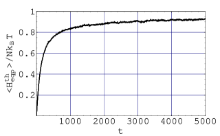
Figure 7: $\langle H^{th}_{epq}\rangle/Nk_{B}T$ vs. t. $\nu=0.003$.

Figure 8: Lattice soliton profiles: pulse shape (a), kink shape (b). Solid line: noisy shape, Dashed line: shape in the presence of damping only. $T=5\times 10^{-5}$, v(0)=1.003, $\nu=0.003$ and $t=5000$

From the generalized equipartition theorem Huang we have that

$$\left\langle\sum_{n=1}^{N}Y_{n}(t)\frac{\partial H(t)}{\partial Y_{n}(t)}\right\rangle=N\,k_{B}\,T$$ (109)

when the system is in thermal equilibrium with an external bath at temperature $T$. The relation (109) is strictly satisfied in the harmonic limit of the Hamiltonian (II), namely $A=0$. For finite values of $A$ the relation (109) is a rather good approximation to evaluate the temperature of our system when the relative displacements are sufficiently small, namely

$$Y_{n+1}(t)-Y_{n}(t)<<\frac{3}{2A}.$$ (110)

Notice that $A=1$ in our simulations. The condition (110) can be obtained by comparing the harmonic term with the cubic anharmonicity in (II) and it is always satisfied in the present work.

So, in order to examine the thermalization process, one can define the ensemble average

$$\langle H_{eqp}(t)\rangle=\left\langle\sum_{n=1}^{N}Y_{n}(t)\frac{\partial H(t)}{\partial Y_{n}(t)}\right\rangle.$$ (111)

For finite times $\langle H_{eqp}(t)\rangle$ possesses two contributions, one due to the coupling to the thermal bath, $\langle H_{eqp}^{th}(t)\rangle$, and the other one due to the soliton, $\langle H_{eqp}^{sol}(t)\rangle$. So

$$\langle H_{eqp}(t)\rangle=\langle H_{eqp}^{th}(t)\rangle+\langle H_{eqp}^{sol}(t)\rangle,$$ (112)

Notice that for a very large system ($N>>1500$) the contribution of the soliton energy, $\langle H_{eqp}^{sol}(t)\rangle$, can be neglected. However, in our system of 1500 sites this contribution is appreciable. In fact, the time evolution of $\langle H_{eqp}(t)\rangle$ for different initial soliton energies presents different values due to the soliton contribution. Here, we remark that in thermal equilibrium, i.e. $t\rightarrow\infty$, these differences vanish. In Eq. (112) $\langle H_{eqp}^{th}(t)\rangle$ gives us information about the time evolution of the temperature of the system in terms of the temperature of the thermal bath. The soliton contribution $\langle H_{eqp}^{sol}(t)\rangle$ can be evaluated numerically using Eq. (111) when the soliton propagates in the presence of the damping but without noise. Then one can perform the numerical subtraction $\langle H_{eqp}(t)\rangle-\langle H_{eqp}^{sol}(t)\rangle$ to obtain $\langle H_{eqp}^{th}(t)\rangle$, which is shown in a normalized form in Fig. 7. We remark that we observe the same result here in systems with the double number of sites, namely 3000. The normalized thermalization process depends only on the damping constant which has the same value $\nu=0.003$ in all our simulations. Notice that for times $t\,{}^{<}_{\sim}\,3/\nu=1000$ there is a fast relaxation process, but for larger times, $t\,{}^{>}_{\sim}\,3/\nu$, the energy system approaches very slowly its stationary value. The thermal equilibrium of the system with the external bath corresponds to the case $\langle H_{eqp}^{th}(t)\rangle/k_{B}T=1$.

Appendix E Profiles

In Fig. 8 we compare snapshots of the system at $t=5000$ with and without noise and in the presence of damping. Figs. 8a and 8b correspond to both the kink shape (absolute displacements) and the pulse shape (relative displacements), respectively. Both shapes, with and without noise, in Fig. 8b were reconstructed from the shapes in Fig. 8a, respectively, by using the algorithm (45).

References

- (1) P.S. Lomdahl, W. C. Kerr, Phys. Rev. Lett., 55, 1235 (1985).
- (2) A. F. Lawrence, J. C. McDaniel, D. B. Chang, B. M. Pierce, R. R. Birge, Phys. Rev. A 33, 1188 (1986).
- (3) M. Toda, Theory of Nonlinear Lattices (Spring-Verlag, 1981).
- (4) Singularities Dynamical Systems, edited by S. N. Pnevmatikos (North-Holland, 1985).
- (5) A. S. Davydov, solitons in Molecular Systems (Reidel, 1985).
- (6) M. A. Collins, Chem. Phys. Lett. 77,342 (1981)
- (7) D. Hochstrasser, F. G. Mertens and H. Büttner, Phys. Rev. A 40, 2602 (1989).
- (8) S. Yomosa, Phys. Rev. A 32, 1752 (1985).
- (9) P. Perez and N. Theodorakopoulos, Phys. Lett. A 117, 405 (1986).
- (10) P. Perez and N. Theodorakopoulos, Phys. Lett. A 124, 267 (1987).
- (11) A. Neuper and F. G. Mertens, in Nonlinear Excitations in Biomolecules, edited by M. Peyrard (Les Editions de Physique, Springer, 1995).
- (12) V. Muto, P.S. Lomdahl and P.L. Christiansen, Phys. Rev. A 42, 7452 (1990).
- (13) A. M. Samsonov, Strain Solitons in Solids and How to Construc them (Chapman & Hall/CRC, 2001)
- (14) V. Konotop and L. Vazquez, Nonlinear Random waves (World Scientific, 1994).
- (15) M. Wadati, J. Phys. Soc. Jpn. 52, 2642 (1983).
- (16) M. Wadati and Y. Akutsu, J. Phys. Soc. Jpn. 53, 3342 (1984).
- (17) R. L. Herman, J. Phys. A 23, 1063 (1990).
- (18) T. Iizuka, Phys. Lett A 181, 39 (1993).
- (19) M. Scalerandi, A. Romano and C. A. Condat, Phys. Rev. E 58 4166 (1998).
- (20) M. Remoissenet Waves Called Solitons (Springer,1996).
- (21) T. Kamppeter, F.G. Mertens, E. Moro, A. Sanchez, A. R. Bishop, Phys. Rev. B 59, 11349 (1999).
- (22) M. Meister, F. G. Mertens, J. Phys. A 33, 2195 (2000).
- (23) M. Meister, F. G. Mertens, and A. Sánchez, Eur. Phys. B 20, 405 (2001).
- (24) L. D. Landau and E. M. Lifshitz, Theory of Elasticity (Pergamon Press, 1986).
- (25) B. Schmittmann and R. K. P. Zia, Statistical Mechanics of Driven Diffusive Systems (Academic Press, 1995).
- (26) K. Nozaki, J. Phys. Soc. Jpn. 56, 3052 (1987).
- (27) A. Orlowski, Phys. Rev. E 49, 2465 (1994).
- (28) E. Arévalo, Yu. Gaididei and F. G. Mertens, Eur. Phys. J. B 27, 63 (2002).
- (29) R. Grimshaw and H. Mitsudera, Stud. Appl. Math. 90, 75 (1993).
- (30) N. R. Quintero, A. Sánchez, F. G. Mertens, Phys. Rev. E 62, 5695 (2000).
- (31) F. G. Mertens, H. J. Schnitzer, and A. R. Bishop, Phys. Rev. B 56, 2510 (1997).
- (32) E. Mann, J. Math. Phys. 38, 3772 (1997).
- (33) C. W. Gardiner, Stochastic Methods (Springer-Verlag, 1990).
- (34) F. Kh. Abdullaev, Physics Reports 179, 1 (1989).
- (35) Peter E. Kloeden, Eckhard Platen, Numerical solution of Stochastic Differential Equations (Springer-Verlag, 1992).
- (36) N. R. Quintero, A, Sánchez, F. G. Mertens, Eur. Phys. B 16, 361 (2000).
- (37) A. Cenian and H. Gabriel, J. Phys.: Condens. Matter 13 1 (2001).
- (38) K. Laasonen, S. Wonczak, R. Strey and A. Laaksonen J. Chem. Phys. 113 9741 (2000).
- (39) Taniuti T. and Wei C., Phys. Soc. Jap. 21, 209 (1968).
- (40) K. Huang, Statistical Mechanics, 2nd ed. (John Wiley and Sons, 1987).