Experimental properties of Bose-Einstein condensates in 1D optical lattices: Bloch oscillations, Landau-Zener tunneling and mean-field effects

Abstract

We report experimental results on the properties of Bose-Einstein condensates in 1D optical lattices. By accelerating the lattice, we observed Bloch oscillations of the condensate in the lowest band, as well as Landau-Zener (L-Z) tunneling into higher bands when the lattice depth was reduced and/or the acceleration of the lattice was increased. The dependence of the L-Z tunneling rate on the condensate density was then related to mean-field effects modifying the effective potential acting on the condensate, yielding good agreement with recent theoretical work. We also present several methods for measuring the lattice depth and discuss the effects of the micromotion in the TOP-trap on our experimental results.

I Introduction

In a very short time after their first observation, Bose-Einstein condensates (BECs) have advanced from being mere physical curiosities to the status of well-studied physical systems [1]. A host of diverse and interesting phenomena such as collective modes, quantized vortices, and solitons, to name but a few, have been extensively investigated and are now well understood [2, 3, 4, 5, 6]. Going from the harmonic potentials used in the experiments mentioned above to optical lattices [7] constitutes a natural extension of the experimental efforts to periodic potentials and has opened up new avenues for research. So far, experiments using periodic potentials have focused mainly on Bragg scattering [8, 9, 10] and, more recently, on phase properties, involving such intriguing concepts as number squeezing [11] and the Mott insulator transition [12, 13]. Some interesting work has also been done on superfluid properties of BECs in optical lattices [14, 15].

In the present work we report on experiments with Bose-Einstein condensates adiabatically loaded into one-dimensional optical lattices [16, 17]. In particular, we look at the dynamics of the BEC when the periodic potential provided by the optical lattice is accelerated, leading to Bloch oscillations and L-Z tunneling. We then proceed to use L-Z tunneling as a tool for measuring the effects of the mean-field interaction between the atoms in the condensate. The modification of the L-Z tunneling rate in the presence of interactions can be interpreted in terms of an effective potential, and we obtain good qualitative agreement with a recent theoretical study using this approach [18].

This paper is organized as follows: After briefly introducing some essential ideas and terminology used in the theoretical treatment of cold atoms in optical lattices (Sec. II), we describe our experimental apparatus in Sec. III. After presenting in Sec. IV the results of preliminary experiments on the calibration of the lattice and on the effects of the condensate micromotion, we turn to the subject of Bloch oscillations in accelerated lattices in Sec. V. The following section VI deals with L-Z tunneling and leads on to a discussion of mean-field effects in Sec. VII. In Sec. VIII we present our conclusions and an outlook on further studies, followed by an Appendix in which we discuss various parameters relevant to the description of our system as an array of tunneling junctions.

II Cold atoms in periodic structures: basic concepts

The properties of cold atoms in conservative optical lattices (i.e. far-detuned, so spontaneous scattering is negligible) bear a strong resemblance to the behaviour of electrons in crystal lattices in condensed matter physics and have, therefore, enjoyed increasing interest since the early days of laser cooling. There are a number of excellent review papers on the subject [19, 20], so in the following we shall only briefly review some basic concepts and establish conventions and notations for the remainder of this work.

The physical system we are considering consists of a Bose-Einstein condensate in a periodic potential created by two interfering linearly polarized laser beams with parallel polarizations. The potential seen by the atoms stems from the ac-Stark shift created by an off-resonant interaction between the electric field of the laser and the atomic dipole. This results in an optical lattice potential of the form

$$U(x)=U_{0}\sin^{2}(\pi x/d),$$ (1)

where $d$ is the distance between neighbouring wells (lattice constant) and

$$U_{0}=(2/3)\hbar\Gamma(I/I_{0})(\Gamma/\Delta),$$ (2)

is the depth of the potential [19], where $I$ is the intensity of one laser beam, $I_{0}$ is the saturation intensity of the ${}^{87}\mathrm{Rb}$ resonance line, $\Gamma$ is the decay rate of the first excited state, and $\Delta$ is the detuning of the lattice beams from the atomic resonance. If the momentum spread of the atoms loaded into such a structure is small compared to the characteristic lattice momentum $p_{B}=2\hbar\pi/d$, then their thermal de Broglie wavelength will be large compared to the lattice spacing $d$ and will, therefore, extend over many lattice sites. The condensates used in our experiment have coherence lengths comparable to their spatial extent of $\approx 10\,\mathrm{\mu m}$, which should be compared to typical lattice spacings in the region of $0.4-1.6\,\mathrm{\mu m}$. A description in terms of a coherent delocalized wavepacket within a periodic structure is then appropriate and leads us directly to the Bloch formalism first developed in condensed matter physics. As will be explained in the following section, we could vary the lattice spacing $d$ by changing the angle between the lattice beams. In this article, the lattice spacing $d$ always refers to the respective geometries of the optical lattices used.

In a lattice configuration in which the two laser beams with wavevector $k_{L}$ are counter-propagating, the usual choices of units are the recoil momentum $p_{rec}=\hbar k_{L}=mv_{rec}$ and the recoil energy $E_{rec}=\hbar^{2}k_{L}^{2}/2m$. In the case of an angle-geometry, with the angle $\theta$ between the lattice beams (see Fig. 1), it is more intuitive to base the natural units on the lattice spacing $d=\frac{\pi}{k_{L}\sin(\theta/2)}$ and the projection $k=\pi/d$ of the laser wavevector $k_{L}$ onto the lattice direction. One can then define a Bloch momentum $p_{B}=2\hbar\pi/d=mv_{B}$, corresponding to the full extent of the first Brillouin zone or, alternatively, to the net momentum exchange in the lattice direction between the atoms and the two laser beams. Possible choices for the energy unit are either the Bloch energy defined as $E_{B}=\hbar^{2}(2\pi)^{2}/md^{2}$, or an ‘effective’ recoil energy $E_{rec}(\theta)=E_{B}/8$, where the parameter $\theta$ indicates the dependence on the lattice geometry [21]. As an intuitive choice for the natural units for the lattice depths is the geometry dependent recoil energy $E_{rec}(\theta)$, we shall quote the lattice depth $U_{0}$ in units of this scaled recoil energy; for simplicity of notation we shall write $E_{rec}$, where it is understood that this always refers to the respective lattice geometries. In Sec. IV on the calibration of the lattice depth, we also use the parameter $s=U_{0}/E_{rec}$. Throughout the paper, velocities and momenta will be quoted in units of the Bloch momentum $p_{B}$ and Bloch velocity $v_{B}$.

In the tight-binding limit ($U_{0}\gg 10\,E_{rec}$), the condensate in the lattice can be approximated by wavepackets localized at the individual lattice sites (Wannier states). This description is more intuitive than the Bloch picture in the case of experiments in which the condensate is released from a (deep) optical lattice into which it had previously been loaded adiabatically. In the present work, this description is only made use of in Sec. 3 and in the Appendix, where the Wannier states are approximated by Gaussian functions.

III Experimental Setup

Our apparatus for creating Bose-Einstein condensates is described in detail in [23]. Briefly, we use a double-MOT setup in order to cool and capture ${}^{87}\mathrm{Rb}$ atoms and transfer them into a time-orbiting potential (TOP) trap. Starting with a few times $10^{7}$ atoms in the magnetic trap, we evaporatively cool the atoms down to the critical temperature for condensation in $\approx 30\,\mathrm{s}$, obtaining pure condensates containing up to $2\times 10^{4}$ atoms. After condensation, the magnetic trap is adiabatically relaxed to mean trap frequencies $\bar{\nu}_{trap}$ on the order of $20-60\,\mathrm{Hz}$, resulting in a variation of the condensate peak density between $2\times 10^{13}\,\mathrm{cm^{-3}}$ and $10^{14}\,\mathrm{cm^{-3}}$  .

The optical lattice was realized using two linearly polarized Gaussian beams (waist $\approx 1.8\,\mathrm{mm}$, maximum power $\approx 3\,\mathrm{mW}$) independently controlled by two acousto-optic modulators (AOMs) and detuned by about $30-60\,\mathrm{GHz}$ above or below the rubidium resonance line. The lattice constant $d$ could be varied through the angle $\theta$ between the laser beams, as shown in Fig. 1. Both horizontal and vertical optical lattices with various angles $\theta$ were realized. Furthermore, by introducing a frequency difference $\delta$ between the two beams, the lattice could be moved at a constant velocity $v_{lat}=\frac{\lambda}{2\sin(\theta/2)}\delta$ or accelerated with an acceleration $a=\frac{\lambda}{2\sin(\theta/2)}\frac{d\delta}{dt}$. While in the countere-propagating geometry lattice depths up to $\approx 2\,E_{rec}$ were realized, in the angle-geometry lattice depths up to $\approx 20\,E_{rec}$ could be realized.

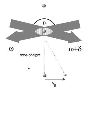
FIG. 1.: Schematic of the experimental procedure. The condensate is loaded into the optical lattice, which can transfer momentum to it in units of $p_{B}=mv_{B}$. The frequency difference $\delta$ between the lattice beams can be used to create a moving or uniformly accelerated lattice.

IV Preliminary Experiments

In order better to understand the effect of the lattice on the condensate and to calibrate the theoretically calculated lattice depth against experimental values, we performed a series of preliminary experiments in conditions in which we expected mean-field effects to be negligible, i.e. either with the condensate in a weak magnetic trap (after adiabatic relaxation), resulting in a low condensate density, or by loading the condensate into the lattice after switching off the magnetic trap. In the latter case, for horizontal lattice configurations the condensate was in free fall after switching off the TOP-trap, limiting the interaction time with the lattice to $10-15\,\mathrm{ms}$. In all experiments, the condensate was observed after $10-20\,\mathrm{ms}$ of time-of-flight by flashing on a resonant imaging beam for $20\,\mathrm{\mu s}$ and observing the shadow cast by the condensate onto a CCD-camera.

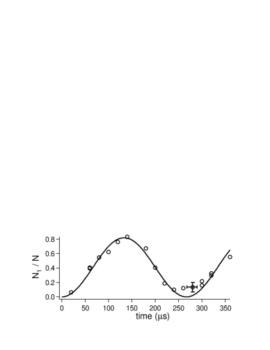
FIG. 2.: Rabi oscillations of the condensate in an optical lattice. Shown here is the fraction $N_{1}/N$ of condensate atoms in the first diffraction order as a function of time. The lattice (in the counter-propagating configuration) was moving with a constant velocity $v=\frac{1}{2}v_{B}$. From the Rabi period $\tau_{Rabi}\approx 260\,\mathrm{\mu s}$ one finds a lattice depth $U_{0}\approx 2\,E_{rec}$.

A Calibration of the lattice

1 Rabi oscillations

If we abruptly switch on an optical lattice moving at a speed $\frac{1}{2}v_{B}$, then in the band-structure picture the condensate finds itself at the edge of the Brillouin zone where the first and second band intersect at zero lattice depth. Raising the lattice up to a final depth of $U_{0}$ opens up a band-gap of width $\Delta E=U_{0}/2$ in the shallow lattice limit, and hence the populations of the two bands [24] accumulate a phase difference $\Delta\phi=\frac{U_{0}}{2\hbar}t$, which results in the two populations getting back into phase (modulo $2\pi$) after a time $\tau_{\rm Rabi}=\frac{2h}{U_{0}}$. In the rest frame of the laboratory, one observes Rabi oscillations [8] between the momentum classes $|p=0\rangle$ and $|p=p_{B}\rangle$ in the shape of varying populations of the corresponding diffraction peaks observed after a time-of-flight (see Fig. 2). From the oscillation frequency $\Omega_{R}$ we could then calculate the lattice depth $U_{0}=2\hbar\Omega_{R}$, yielding results that fell short by about $20-25$ percent of the calculated value. We attribute the discrepancy between the experimental and theoretical values mainly to the uncertainty in our laser intensity measurements and to imperfections in the lattice beam cross-section and polarization.
As pointed out in [19], an alternative way of interpreting the observed Rabi oscillations in this kind of experiment is to consider a two-photon Raman coupling between the two momentum states, whose energies differ by $\Delta E=2\hbar^{2}k^{2}/m=4E_{rec}$. The coupling is resonantly enhanced if the frequency difference $\delta$ between the two lattice beams matches $\Delta E/h$, i.e. if the lattice velocity $v_{lat}=\frac{\lambda}{2}\delta=\frac{\hbar k}{m}=\frac{1}{2}v_{B}$, as before. The two-photon Rabi frequency for the beam intensities corresponding to a lattice depth $U_{0}$ can be easily calculated and, again, gives $\Omega_{R}=U_{0}/2\hbar$.

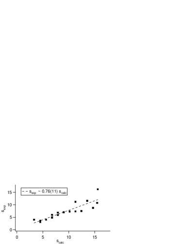
FIG. 3.: Calibration of the lattice depth by measuring the side-peak populations. We calculated the lattice depth from the mean value of the plus and minus first order side-peak using Eqn. 3. By varying the intensity of the lattice beams, we performed measurements of $s_{exp}$ for various values of $s_{calc}$.

2 Analysis of the interference pattern

If the depth of a stationary lattice is increased on a timescale comparable to the inverse of the chemical potential of the condensate (in frequency units), then the condensate can adiabatically adapt to the presence of the periodic potential [25]. When the lattice has reached its final depth, the system is in a steady state with the condensate distributed among the lattice wells (in the limit of a sufficiently deep lattice in order for individual lattice sites to have well-localized wavepackets). If the lattice is now switched off suddenly, the individual (approximately) Gaussian wavepackets at each lattice site will expand freely and interfere with one another. (In this case a tight-binding approximation is more intuitive than a Bloch wave approach.) The resulting spatial interference pattern after a time-of-flight of $t$ will be a series of regularly spaced peaks with spacing $v_{B}t$, corresponding to the various diffraction orders, with a Gaussian population envelope of width $\approx\hbar t/m\sigma$, where $\sigma$ is the width of the wavepackets at the individual lattice sites. In particular, Pedri et al. have shown [26] that the relative populations $P_{\pm 1}$ of the two symmetric plus and minus first order peaks with respect to the zeroth-order central peak are given by $P_{\pm 1}=\exp(-4\pi^{2}\sigma^{2}/d^{2})$ [27]. For deep lattice wells, $\sigma/d$ can be found by making a harmonic approximation to the sinusoidal lattice potential about a potential minimum, giving a Gaussian width $\sigma=d/\pi s^{1/4}$. For the relatively shallow lattice used in our experiments ($s<20$), however, this approximation is not very accurate. Instead, we used a variational ansatz for a Gaussian wavepacket in a sinusoidal potential. The resulting transcendental equation can be solved numerically to yield $\sigma$ (see Ref. [26] and Appendix). Alternatively, we can find an analytical expression for the lattice depth as a function of the measured side-peak population, giving

$$s_{exp}=\frac{16}{[\ln(P_{\pm 1})]^{2}}P_{\pm 1}^{-1/4}.$$ (3)

This expression can be used directly to calibrate the lattice based on a measurement of the side-peak populations. Figure 3 shows the lattice depth $s_{exp}$ as inferred from the above equation by measuring the populations of the zeroth and plus/minus first order diffraction peaks plotted against the lattice depth $s_{calc}$ calculated from the beam intensity and detuning, taking into account the losses at the cell windows ($\approx 8$ percent). A straight line fit gives $s_{exp}=(0.76\pm 0.1)s_{calc}$, consistent with the results obtained by measuring the Rabi oscillation frequency.

FIG. 4.: Calibration of the lattice potential with $d=1.2\mu$m by measuring the tunneling rate. Plotted here as a function of the calculated lattice depth $s_{calc}$ is the number of condensate atoms $N_{trapped}$ remaining in the lattice at time $t_{lat}=10.1\,\mathrm{ms}$ after switching off the magnetic trap. Fitting a theoretical curve (see text) to the data we find that $s_{exp}\approx 0.76\times s_{calc}$, consistent with the results of the other calibration techniques.

3 Tunneling

If the lattice beams are arranged such as to create a periodic potential along the vertical direction, for deep enough lattice potentials the condensate can be held against gravity for several hundred milliseconds. As the potential is reduced below a critical depth the condensate starts tunneling out of the lattice. If this critical depth is fairly small ($\lesssim 12\,E_{rec}$), then the tunneling rate can be calculated from L-Z theory. If the condensate moving with the acceleration $a$ crosses the band gap $\Delta E$ at the Brillouin zone edge fast enough, the probability $r$ for undergoing a transition to the first excited band is given by [28]

$$r=e^{-a_{c}/a},$$ (4)

with the critical acceleration

$$a_{c}=\frac{d}{4\hbar^{2}}(\Delta E)^{2}.$$ (5)

If the atoms can tunnel into the second band and, therefore, effectively into the continuum, they will no longer be trapped by the lattice. Starting from this assumption, for the condensate accelerated by gravity with $a=9.81\,\mathrm{m\,s^{-2}}$ we can calculate $N_{trapped}$ the number of atoms that remain trapped after a time $t_{lat}$ to be

$$N_{trapped}=N_{ini}(1-r)^{t_{lat}/\tau_{B}},$$ (6)

where $t_{lat}$ is an integer multiple of the Bloch period $\tau_{B}=v_{B}/g$ (see next section). Figure 4 shows the results of an experiment in which the condensate was loaded into a vertical lattice with lattice constant $d=1.2\,\mathrm{\mu m}$, after which the magnetic trap was switched off and the number of trapped atoms was determined after a time $t_{lat}=10.1\,\mathrm{ms}=26\,\tau_{B}$ as a function of $s_{calc}$. Fitting the above equation for $N_{trapped}(t)$ to the data, we found that the actual lattice depth was around $75$ percent of the value calculated from the lattice beam parameters. This value agrees with those found using Rabi oscillations and side-peak intensity.

B Effects of the micromotion

The time-orbiting potential trap used in our experiments is an intrinsically dynamic trap which relies on the fast rotation of the bias field to create an averaged harmonic trapping potential. It has been shown, however, that the atoms in such a trap perform a small but non-negligible micromotion at the rotation frequency $\Omega_{TOP}$ ($2\pi\times 10\,\mathrm{kHz}$ in our set-up) of the bias field [29]. Although the spatial amplitude of this fast motion is extremely small (less than $100\,\mathrm{nm}$ for typical experimental parameters), its velocity can be as large as a few millimeters per second. As the Bloch velocities $v_{B}$ of the lattices used in our experiments lie between $3\,\mathrm{mm\,s^{-1}}$ and $11.8\,\mathrm{mm\,s^{-1}}$ (depending on the angle $\theta$), the micromotion velocity component along the lattice direction can be a significant fraction of the Bloch velocity. This has two consequences:
(a) If the interaction time of the lattice with the condensate is short compared to $2\pi/\Omega_{\mathrm{TOP}}=100\,\mathrm{\mu s}$, the initial velocity of the condensate is undetermined to within the micromotion velocity amplitude.
(b) If, on the other hand, the interaction time with the lattice is long compared with $2\pi/\Omega_{\mathrm{TOP}}$, the condensate oscillates to and fro in the Brillouin zone and can, if the micromotion velocity is large enough, reach the band edge and thus be Bragg-reflected. Another possible mechanism is the parametric excitation at $\Omega_{TOP}$ of transitions to higher bands.

All of these effects are undesirable if one wants to conduct well-controlled experiments. In our setup, the micromotion takes place in the horizontal plane and was thus important when we worked with horizontal lattices. In order to minimize the detrimental effects of the micromotion, we employed two techniques:
(a) For short interaction times, we synchronized the instant at which the lattice was switched on with a given phase of the rotating bias field. This allowed us to ensure that the lattice was always switched on when the condensate velocity along the lattice direction was approximately zero. A small residual jitter, however, was still given by the sloshing (dipole oscillation) of the condensate in the magnetic trap, which was especially critical when we worked with large lattice constants (and hence small Bloch velocities).
(b) For long interaction times, we phase-modulated one of the lattice beams synchronously with the rotating bias field and with a modulation depth that resulted in the lattice ‘shaking’ with the same velocity amplitude as the micromotion. In this way, in the rest-frame of the lattice the condensate was stationary (again, save a possible sloshing motion).

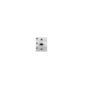
FIG. 5.: Effects of the micromotion in a horizontal counter-propagating lattice configuration. (a) shows a condensate (after a time-of-flight of $15\,\mathrm{ms}$) released from the magnetic trap with $\overline{\nu}_{trap}=25\,\mathrm{Hz}$ without the optical lattice. In (b), the optical lattice($U_{0}\approx 2\,E_{rec}$) was switched on for $7.5\,\mathrm{ms}$ with the magnetic trap still on. One clearly sees that the condensate is broadened along the lattice direction. In (c), we compensated the micromotion by phase-modulating one of the lattice beams (see text). The difference in intensity of the dark spot in (a) and (c) is due to shot-to-shot fluctuations of the number of atoms in the condensate. Also, in (c) a faint spot to the left of the central condensate can be seen; this corresponds to a part of the condensate having undergone Bragg reflection due to an initial sloshing.

Figure 5 shows the effect of method (b) in which a condensate was loaded into a lattice ($U_{0}\approx 2\,E_{rec}$) with a $1\,\mathrm{ms}$ ramp and then left in the lattice for $7.5\,\mathrm{ms}$ before the latter was suddenly switched off. When the micromotion was not compensated by phase-modulating one of the lattice beams, the condensate appeared ‘smeared out’ when observed after a time-of-flight. Using the compensation technique eliminated this effect (Fig. 5 (c)).

FIG. 6.: Acceleration of a Bose-Einstein condensate in the counter-propagating geometry ($d=0.39\,\mathrm{\mu m}$). In (a)-(f) the lattice parameters were $U_{0}=2.3\,E_{rec}$ and $a=9.81\,\mathrm{m\,s^{-2}}$, and the condensate was accelerated for $0.1,0.6,1.1,2.1,3.0$ and $3.9\,\mathrm{ms}$, respectively. In (g), the condensate was accelerated for $2.5\,\mathrm{ms}$ with the same lattice depth as above, but with $a=25\,\mathrm{m\,s^{-2}}$. In this case, a fraction of the condensate underwent L-Z tunneling out of the lowest band each time a Bragg-resonance was crossed. Note that the separations between the spots vary because detection occurred after different times-of-flight.

V Bloch oscillations

A Theoretical considerations

One of the most intriguing manifestations of the quantum dynamics of particles in a periodic potential are Bloch oscillations. Their theoretical explanation is based on the evolution in the band-structure picture of a collection of particles occupying a small fraction of the Brillouin zone when the potential is switched on (meaning that in real space their wavefunctions extend over many lattice sites, which translates into temperatures well below the recoil temperature $T_{rec}=E_{rec}/k_{B}$, see Sec. II). If the lattice is switched on adiabatically, then all the atoms will end up in the lowest band. Accelerating the atoms by applying a force (real or inertial) to them will result in their being moved through the Brillouin zone until they reach the band edge. Owing to the effects of the periodic potential, at this point there is a gap between the first and second band, and unless the acceleration is large enough for the atoms to undergo a L-Z transition (see Sec. VI), they will remain in the first band and thus be Bragg-reflected back to the opposite end of the Brillouin zone. In the rest-frame of the lattice this corresponds to the atoms’ velocity oscillating to and fro between $+\frac{1}{2}\alpha v_{B}$ and $-\frac{1}{2}\alpha v_{B}$ (where $0<\alpha<1$, depending on the lattice depth), whereas in the laboratory frame these Bloch oscillations manifest themselves as an undulating (or, for shallow lattices, almost stepwise) increase in velocity rather than the linear increase expected in the classical picture in which the atoms are ‘dragged along’ by the potential. The instantaneous velocity of the atomic wavepacket in the lattice frame can be calculated from the slope of the first band at the corresponding quasi-momentum $q$, giving $v=\frac{1}{\hbar}\frac{dE(q)}{dq}$.

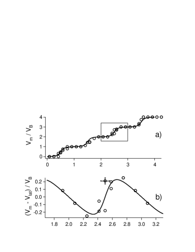
FIG. 7.: Bloch oscillations of the condensate mean velocity $v_{m}$ in an optical lattice. (a) Acceleration in the counter-propagating lattice with $d=0.39\,\mathrm{\mu m}$, $U_{0}\approx 2.3\,E_{rec}$ and $a=9.81\,\mathrm{m\,s^{-2}}$. Solid line: theory. (b) Bloch oscillations in the rest frame of the lattice, along with the theoretical prediction (solid line) derived from the shape of the lowest Bloch band.

B Experimental results

The condensate was loaded into the (horizontal) optical lattice with lattice constant $d=0.39\,\mathrm{\mu m}$ immediately after switching off the magnetic trap. The switch-on was done adiabatically with respect to the lattice vibration frequencies [7] $\omega_{vib}=2E_{rec}\sqrt{s}/\hbar$ (valid for $s\gg 1$) by ramping up the lattice beam intensity over a time $t_{ramp}\approx 100\,\mathrm{\mu s}$. Thereafter, the lattice was accelerated with $a=9.81\,\mathrm{m\,s^{-1}}$ by ramping the frequency difference $\delta$ between the beams. After a time $t_{accel.}$ the lattice was switched off and the condensate was observed after an additional time-of-flight of $13-18\,\mathrm{ms}$. Figure 6 shows the results of these measurements in the laboratory frame. The Bloch oscillations are more evident, however, if one calculates the mean velocity $v_{m}$ as the weighted sum over the momentum components after the interaction with the accelerated lattice, as shown in Fig. 7. When the instantaneous lattice velocity $v_{lat}$ is subtracted from $v_{m}$, one clearly sees the oscillatory behaviour of $v_{m}-v_{lat}$. This result is analogous to the first observation of Bloch oscillations in cold atoms at sub-recoil temperatures [19]. The added feature in our experiment is that by using a Bose-Einstein condensate released from a weak magnetic trap, the spatial extent of the atomic cloud is sufficiently small so that after a relatively short time-of-flight ($\approx 10-20\,\mathrm{ms}$) the separation between the individual momentum classes is already much larger than the size of the condensate due to its expansion and can, therefore, be easily resolved. The mean velocity is then calculated simply by counting the number of atoms in each of these classes (the dark dots visible in Fig. 6).

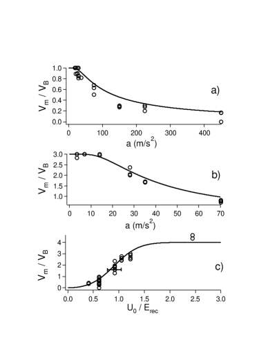
FIG. 8.: L-Z tunneling of a condensate in an optical lattice. (a) and (b): Mean velocity of the condensate after acceleration of the lattice to $v_{B}$ and $3v_{B}$, respectively, as a function of acceleration. (c) Mean velocity of the condensate after acceleration of the lattice to $4.4v_{B}$ as a function of lattice depth. In (a) and (b), the lattice depth was fixed at $U_{0}=2\,E_{rec}$, and in (c) the acceleration $a=9.81\,\mathrm{m\,s^{-1}}$. In (c), agreement with theory is expected to be somewhat less good because the final velocity of the lattice is not an integer multiple of $v_{B}$ (see text).

VI L-Z tunneling

We investigated the $U_{0}$ dependence for the L-Z tunneling of the condensate into the second band when crossing the edge of the Brillouin zone, and therefore, effectively to the continuum, as the gaps between higher bands were negligible for the shallow potentials used in our experiments. As in Sec. V, we loaded the condensate into the optical lattice after switching off the magnetic trap. The trap had been adiabatically expanded to a mean trap frequency $\overline{\nu}_{trap}\approx 20\,\mathrm{Hz}$ prior to switch-off, thus ensuring that the condensate density was small ($<10^{13}\,\mathrm{cm^{-3}}$) and, therefore, mean-field effects could be neglected. After that, the lattice was accelerated to a final velocity $nv_{B}$ ($n=1,2,...$). Each time the condensate was accelerated across the edge of the Brillouin zone, according to L-Z theory a fraction $r$ (see Eqns. 4 and 5) underwent tunneling into the first excited band. In Fig. 8, the average velocity of the condensate after the acceleration is shown as a function of $a$ and $U_{0}$ along with theoretical predictions using the L-Z tunneling probability. If the final lattice velocity is $v_{B}$, one finds a final mean velocity $v_{m}=(1-r)v_{B}$, whereas a straightforward generalization of this formula yields

$$v_{m}=v_{B}(1/r-1)[1-(1-r)^{n}]$$ (7)

for a final lattice velocity of $nv_{B}$. In this case, a fraction $r$ of the condensate undergoes L-Z tunneling each time the Bragg resonance is crossed, with a remaining fraction $1-r$ being accelerated further. Note that this result is only independent of the lattice depth (except through the tunneling fraction $r$) if the final lattice velocity is an integer multiple of $nv_{B}$. As can be seen from Fig. 8, agreement with theory is good. Again, it should be stressed here that owing to the small condensate densities, these measurements do not differ qualitatively from those using cold but uncondensed atoms [19].

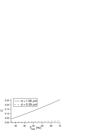
FIG. 9.: Calculated dependence of the parameter $C$ on the trap frequency $\bar{\nu}_{trap}$ for two different lattice configurations. Mean-field effects are far more important for the larger lattice constant $d=1.56\,\mathrm{\mu m}$, which results in a $C$ larger by a factor of $\approx 16$ with respect to the counter-propagating configuration ($d=0.39\,\mathrm{\mu m}$). In calculating $C$, we assumed a typical condensate number $N_{tot}=10^{4}$ and used the Thomas-Fermi expression for the condensate peak density.

VII Mean-field effects

A Theoretical considerations

In Bose-Einstein condensates, interactions between the constituent atoms are responsible for the non-linear behaviour of the BEC and can lead to interesting phenomena such as solitons [6] and four-wave mixing with matter waves [30]. As the atoms are extremely cold, collisions between them can be treated by considering only $s$-wave scattering, which is described by the scattering length $a_{s}$. For rubidium the atomic mean-field interaction is repulsive corresponding to a positive scattering length $a_{s}=5.4\,\mathrm{nm}$.

For a BEC in an optical lattice, one expects an effect due to the mean-field interaction similar to the one responsible for determining the shape of a condensate in the Thomas-Fermi limit: The interplay between the confining potential and the density-dependent mean-field energy leads to a modified ground state that reflects the strength of the mean-field interaction. Applied to a BEC in a periodic potential, one expects the density modulation imposed on the condensate by the potential (higher density in potential troughs, lower density where the potential energy is high) to be modified in the presence of mean-field interactions. In particular, the tendency of the periodic potential to create a locally higher density where the potential energy of the lattice is low will be counteracted by the (repulsive) interaction energy that rises as the local density increases.

The nonlinear interaction of the condensate inside an optical lattice with lattice constant $d=\pi/\sin(\theta/2)k_{L}$ may be described through a dimensionless parameter [18]

$$C=\frac{\pi n_{0}a_{s}}{k_{L}^{2}sin^{2}(\theta/2)}=\frac{n_{0}g}{E_{B}},$$ (8)

with $g$ defined in Eqn. (12), corresponding to the ratio of the nonlinear interaction term and the Bloch energy. The parameter $C$ contains the peak condensate density $n_{0}$ [31], the scattering length, and the atomic mass $m$. In our notation, the parameter $C$ always refers to the respective lattice geometries with angle $\theta$. From the dependence of $C$ on the lattice angle $\theta$ it follows that a small angle $\theta$ (meaning a large lattice constant $d$) will result in a large interaction term $C$. In our experiment, creating a lattice with $\theta=29$ deg (i.e. $d=1.56\,\mathrm{\mu m}$) allowed us to realize a value of $C$ larger by a factor of more than $10$ with respect to Ref. [32] using a comparable condensate density. Figure 9 shows our estimates for the nonlinear interaction parameter $C$ realized by varying the magnetic trap frequency (and, thereby, the density $n_{0}$).

In Ref. [18], the authors derived an analytical expression in the perturbative limit (assuming $U_{0}\ll E_{B}$) for the effect of the mean-field interaction on the ground state of the condensate in the lattice. Starting from the Gross-Pitaevskii equation for the condensate wavefunction in a one-dimensional optical lattice (i.e. a one dimensional Hamiltonian equivalent to that of Eq. 11), they found that by substituting the potential depth $U_{0}$ with an effective potential

$$U_{eff}=\frac{U_{0}}{1+4C},$$ (9)

the effect of the mean-field interaction could be approximately accounted for. This reduction of the effective potential agrees with the intuitive picture of the back-action on the periodic potential of the density modulation of the condensate imposed on it by the lattice potential. For repulsive interactions, this results in the effective potential being lowered with respect to the actual optical potential created by the lattice beams.

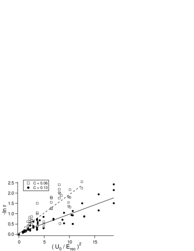
FIG. 10.: L-Z tunneling for different values of the interaction parameter $C$. The tunneling fraction $r$ was measured by accelerating the condensate to $v_{B}$ in a vertical lattice with $d=1.2\,\mathrm{\mu m}$, and $C$ was varied by changing the trap frequency and hence the condensate density $n_{0}$. The straight lines are best linear fits to the data.

B Experimental results

In order to measure the effective potential $U_{eff}$, we assumed that the perturbative treatment described above can be extended to define an effective band gap $\Delta E_{eff}$ at the edge of the Brillouin zone which for a particular interaction parameter $C$ can be written as

$$\Delta E_{eff}=\frac{U_{eff}}{2}=\frac{U_{0}}{2(1+4C)},$$ (10)

where $\Delta E$ is the value of the band gap in the absence of interactions [33]. One can then derive the interaction parameter $C$ indirectly by determining the effective band gap $\Delta E_{eff}$ from the L-Z tunneling rate $r$, using Eqns.(4) and (5) with the band gap $\Delta E_{eff}$.

Figure 10 shows the results of measurements of the L-Z tunneling rate for two different values of $C$. In this experiment, in contrast to those described thus far, the lattice was adiabatically ramped up with the magnetic trap still on in order to maintain the condensate at a constant density. After accelerating the condensate to $v_{B}$, the magnetic trap and the lattice were both switched off and the fraction $r$ that had undergone tunneling (i.e. the fractional population that appeared in the zero momentum class) was measured after a time-of-flight. The effective potentials could be derived from the slopes of the linear fits in Fig. 10 and were found to be markedly different. Comparing the experimentally determined values for $C$ with those calculated on the basis of the experimental parameters, we found that the experimental values were larger by about a factor of $2.5$. In fact, we expected the predictions of [18] to be only approximately valid (see discussion below).

In order further to test the validity of Eqn. 10, we used two different lattice angles $\theta$ and varied the condensate density by changing the trap frequency[35]. The effective potential in each case was inferred from the tunneling probability $r$ for a fixed lattice depth. The results of these measurements are shown in Fig. 11, along with the theoretical predictions. Clearly, the reduction of $U_{eff}$ with respect to the non-interacting limit is much larger for the small lattice angle, as expected from theory. The general behaviour of $U_{eff}$ as a function of $C$ is well reproduced by our results. Replacing $C$ by $\approx 2.5C$ in the formula for $U_{eff}/U_{0}$ leads to much better agreement with the experimental data, which is consistent with the results of Fig. 10.

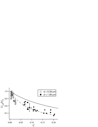
FIG. 11.: Dependence of the effective potential $U_{\rm eff}$ on the interaction parameter $C$. The different symbols indicate the two (horizontal) lattice geometries, with the empty symbols corresponding to the counter-propagating case and the full ones to the angle configuration ($d=1.56\,\mathrm{\mu m}$). Solid line: theoretical prediction of Choi and Niu’s expression for $U_{eff}$. The parameters in these experiments were $a=23.4\,\mathrm{m\,s^{-2}}$ and $U_{0}=2.2\,E_{rec}$ for the counter-propagating lattice and $a=3.23\,\mathrm{m\,s^{-2}}$ and $U_{0}=5.7\,E_{rec}$ for the angle geometry.

In spite of the good qualitative agreement, we should like to point out that the model of Choi and Niu [18] only approximately describes our experiment, as it assumes an infinitely extended condensate and neglects the radial degrees of freedom of the condensate in the one-dimensional lattice. Especially the finite extent of the condensate in our experiment (in which only $6-30$ lattice sites were occupied by the condensate, see the Appendix) should lead to non-negligible corrections. Also, the analysis of Ref. [18] assumes a uniform condensate density across the entire lattice, whereas in our experiment there was a pronounced density envelope over the $6-30$ lattice wells occupied by the condensate. In the above comparison with theory we calculated $C$ using the peak condensate density.

VIII Conclusions and outlook

We have presented experimental results on the adiabatic loading and subsequent coherent acceleration of a Bose-Einstein condensate in a 1D optical lattice. In the adiabatic acceleration limit we have observed Bloch oscillations of the condensate mean velocity in the lattice reference frame, whereas for larger accelerations and/or smaller lattice depths L-Z tunneling out of the lowest band occurred. The experimentally observed variation of the L-Z tunneling rate with the condensate density has been related to the mean-field interaction in the condensate leading to a reduced effective potential. Agreement with recent theoretical results is satisfactory.
A natural extension of our work on mean-field effects will consist in checking theoretical predictions concerning instabilities at the edge of the Brillouin zone [36] and the possibility of creating bright solitons by exploiting the nonlinearity of the Gross-Pitaevskii equation, which can compensate the negative group velocity dispersion at the band edge [37].

IX Acknowledgments

This work was supported by the INFM through a PRA Project, by MURST through the COFIN2000 Initiative, and by the European Commission through the Cold Quantum-Gases Network, contract HPRN-CT-2000-00125. O.M. gratefully acknowledges a Marie-Curie Fellowship from the European Commission within the IHP Programme. The authors thank M. Anderlini for help in the data acquisition.

An array of coupled wells - relevant parameters

The possibility of studying the dynamics of a Bose-Einstein condensate spread out coherently over a large number of wells of a periodic potential, bearing a close resemblance to an array of coupled Josephson junctions, has inspired a host of theoretical papers in the past few years. On the experimental side, phase fluctuations [11], Josephson oscillations [15] and the Mott insulator transition [12] have been investigated, invoking concepts and notations inherited from the physics of Josephson junctions. In order to facilitate the comparison of our work with these studies, in this Appendix we report the values pertinent to our experiment for the various parameters that are important in the description of coherent quantum effects in an array of tunneling junctions.

For the description of a condensate in an array of coupled potentials wells, the physical parameters needed to describe the dynamics of the system are the on-site interaction $E_{C}$, and the tunneling energy $E_{J}$. These quantities are defined in a variety of ways in the literature [38, 39, 40]. Our calculations are based on a variational ansatz of the total Hamiltonian

$$H_{tot}=H_{0}+g|\Psi(\vec{r})|^{2}=\frac{-\hbar^{2}}{2m}\nabla^{2}+U_{0}\sin^{2}(\vec{k_{L}}\cdot\vec{r})+g|\Psi(\vec{r})|^{2},$$ (11)

with the interaction parameter $g$ given by

$$g=4\pi\hbar^{2}a_{s}/m$$ (12)

and the wavefunction $\Psi(\vec{r})$ given by

$$\Psi(\vec{r})=\sum_{n}\psi_{0}(x-nd)\sqrt{N_{n}(t)}e^{i\vartheta_{n}(t)}\phi(y,z).$$ (13)

Here, $N_{n}(t)$ is the number of atoms at site $n$, $\vartheta_{n}(t)$ is a site-dependent phase, and $\phi(y,z)$ is the part of the wavefunction perpendicular to the lattice direction. Basing the variational ansatz for $\psi_{0}$ on a Gaussian of the form $\psi_{0}(x)=\frac{1}{\sigma^{1/2}\pi^{1/4}}\exp[-\frac{1}{2}(x/\sigma)^{2}]$ [42], we obtain a minimum energy wavefunction of width $\sigma$ which, expressed in units of the width $\sigma_{h}=\frac{d}{\pi}(U_{0}/E_{rec})^{-1/4}$ in the harmonic approximation of the potential wells, satisfies the condition

$$\exp\left[-\left(\frac{\sigma}{\sigma_{h}}\right)^{2}/\sqrt{U_{0}/E_{rec}}\right]=\left(\frac{\sigma}{\sigma_{h}}\right)^{-4}.$$ (14)

This equation can be solved numerically to yield $\sigma/\sigma_{h}$.

We now define the quantities $E_{C}$ and $E_{J}$ as follows [41]:

$$E_{C}=N_{s}g_{1\mathrm{D}}\int dx\,\psi_{0}(x)^{4},$$ (15)

$$E_{J}=-\int dx\,\psi_{0}(x)H_{0}\psi_{0}(x-d).$$ (16)

In the expression for $E_{C}$, the 1D interaction parameter $g_{1\mathrm{D}}$ is defined as

$$g_{1\mathrm{D}}=g\frac{1}{\pi\sigma_{y}\sigma_{z}},$$ (17)

where $\sigma_{y,z}$ are the Gaussian widths in the $y$ and $z$ directions of the radial wavefunction

$$\phi(y,z)=\frac{1}{\pi^{1/2}\sigma_{y}^{1/2}\sigma_{z}^{1/2}}\exp[-\frac{1}{2}(y/\sigma_{y})^{2}-\frac{1}{2}(z/\sigma_{z})^{2}].$$ (18)

The 1D coupling strength $g_{1\mathrm{D}}$ is equivalent to that derived by Olshanii in the case of a cigar shaped atomic trap[43]. $N_{s}=N_{tot}/n_{occ}$ is the mean number of atoms per lattice site, with $N_{tot}=\sum_{n}N_{n}$ the total number of condensate atoms and $n_{occ}$ the number of lattice sites occupied, as defined below.

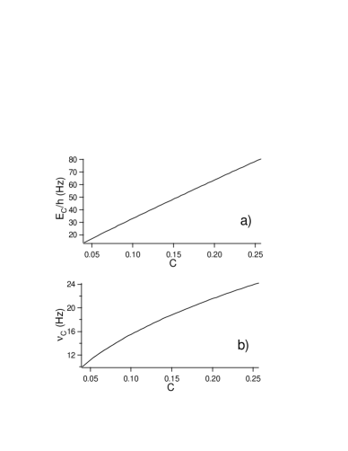
FIG. 12.: Dependence of the on-site interaction energy $E_{C}$, in (a), and of the Josephson frequency $\nu_{C}$, in (b), on the non-linear parameter $C$ for a lattice with $d=1.56\,\mathrm{\mu m}$, $U_{0}=5.6\,E_{rec}$ and $N_{tot}=10^{4}$. For these parameters, the tunneling energy $E_{J}=h\times 8\,\mathrm{Hz}$.

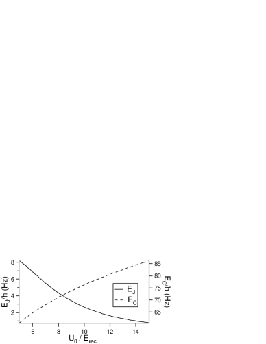
FIG. 13.: Variation of $E_{J}$ and $E_{C}$ with lattice depth (lattice constant $d=1.56\,\mathrm{\mu m}$, $N_{tot}=10^{4}$) for a fixed value of the non-linear parameter $C=0.17$.

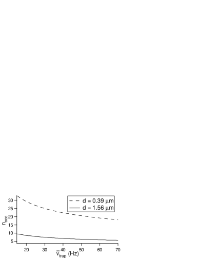
FIG. 14.: Number of wells occupied by the condensate as a function of the magnetic trap frequency for two different lattice constants. For the large lattice constant, the number of wells is small, so that finite-size effects are expected to be important.

As the maximum lattice depth we could experimentally achieve in the counter-propagating configuration was $\approx 2\,E_{rec}$, we have only calculated $E_{C}$ and $E_{J}$ numerically for a lattice in the angle-geometry with $d=1.56\,\mathrm{\mu m}$, as the present model only gives reasonable values for $U_{0}/E_{rec}\gtrsim 4$. Figure 12(a) shows the dependence of the on-site interaction energy $E_{C}$ as a function of the non-linear interaction parameter $C$ for a constant lattice depth $U_{0}=5.6\,E_{rec}$. The Josephson frequency $\nu_{c}=\sqrt{E_{J}E_{C}}/h$ as a function of $C$ is shown in Fig. 12 (b). In Fig. 13, both $E_{J}$ and $E_{C}$ are plotted as a function of the lattice depth.

Finally, we briefly discuss the variation with $\bar{\nu}_{trap}$ of the number $n_{occ}$ of lattice sites occupied by the condensate. In a rough approximation, this number is given by the diameter of the condensate as calculated from the Thomas-Fermi limit divided by the lattice constant $d$. Pedri et al. have used a more refined model [26] to derive the expression

$$n_{occ}=1+\frac{2}{d}\sqrt{\frac{\hbar}{2\pi m\bar{\nu}_{trap}}}\left(\frac{15}{8\sqrt{\pi}}N_{tot}a_{s}\sqrt{\frac{m\pi\bar{\nu}_{trap}}{\hbar}}\frac{d}{\sigma}\right)^{1/5}.$$ (19)

Figure 14 shows $n_{occ}$ as a function of $\bar{\nu}_{trap}$ for two different lattice geometries. It is clear from this plot that in the angle-geometry, the number of wells occupied ($<10$) is small and hence we expect finite-size effects to be particularly important in this configuration.

REFERENCES

- [1] See reviews by W. Ketterle et al., and by E. Cornell et al. in Bose-Einstein condensation in atomic gases, edited by M. Inguscio, S. Stringari and C. Wieman (IOS Press, Amsterdam) (1999).
- [2] M.-O. Mewes, M.R. Andrews, N.J. van Druten, D.M. Kurn, D.S. Durfee, C.G. Townsend, and W. Ketterle, Phys. Rev. Lett. 77, 988 (1996).
- [3] D.S. Jin, M.R. Matthews, J.R. Ensher, C.E. Wieman, and E.A. Cornell, Phys. Rev. Lett. 78, 764 (1997).
- [4] K.W. Madison, F. Chevy, W. Wohlleben, and J. Dalibard, Phys. Rev. Lett. 84, 806 (2000).
- [5] J.R. Abo-Shaeer, C. Raman, J.M. Vogels, and W. Ketterle, Science 292, 5516 (2001).
- [6] S. Burger, K. Bongs, S. Dettmer, W. Ertmer, K. Sengstock, A. Sanpera, G.V. Shlyapnikov, and M. Lewenstein, Phys. Rev. Lett. 83, 5198 (1999).
- [7] For reviews see P.S. Jessen and I.H. Deutsch, Adv. At. Mol. Opt. Phys. 37, 95 (1996); G. Grynberg and C. Triché, in Coherent and Collective Interactions of Particles and Radiation Beams edited by A. Aspect, W. Barletta, and R. Bonifacio (IOS Press, Amsterdam) (1996); D.R. Meacher, Cont. Phys. 39, 329 (1998).
- [8] M. Kozuma, L. Deng, E.W. Hagley, J. Wen, R. Lutwak, K. Helmerson, S.L. Rolston, and W.D. Phillips, Phys. Rev. Lett. 82, 871 (1999); Yu.B. Ovchinnikov, J.H. Müller, M.R. Doery, E.J.D. Vredenbregt, K. Helmerson, S.L. Rolston, and W.D. Phillips, ibid. 83, 284 (1999); J.E. Simsarian, J. Denschlag, M. Edwards, C.W. Clark, L. Deng, E.W. Hagley, K. Helmerson, S.L. Rolston, and W.D. Phillips, ibid. 85, 2040 (2000).
- [9] D.M. Stamper-Kurn, A.P. Chikkatur, A. Görlitz, S. Inouye, S. Gupta, D.E. Pritchard, and W. Ketterle, Phys. Rev. Lett. 83, 2876 (1999).
- [10] R. Ozeri, J. Steinhauer, N. Katz, and N. Davidson, e-print: cond-mat 0112496 (2001).
- [11] C. Orzel, A.K. Tuchman, M.L. Fenselau, M. Yasuda, and M.A. Kasevich, Science 231, 2386 (2001).
- [12] M. Greiner, O. Mandel, T. Esslinger, T.W. Hänsch, and I. Bloch, Nature 415, 6867 (2002).
- [13] D. Jaksch, C. Bruder, J.I. Cirac, C.W. Gardiner, and P. Zoller, Phys. Rev. Lett. 81, 3108 (1998).
- [14] S. Burger, F. Cataliotti, C. Fort, F. Minardi, M. Inguscio, M.L. Chiofalo, and M.P. Tosi, Phys. Rev. Lett. 86, 4447 (2001).
- [15] F.S. Cataliotti, S. Burger, C. Fort, P. Maddaloni, F. Minardi, A. Trombettoni, A. Smerzi, and M. Inguscio, Science 293, 843 (2001).
- [16] Preliminary results were reported in O. Morsch, J.H. Müller, M. Cristiani, D. Ciampini, and E. Arimondo, Phys. Rev. Lett. 87, 140402 (2001).
- [17] Related experiments have been performed by the group of W.D. Phillips; A. Browaeys, private communication (2001).
- [18] D. Choi and Q. Niu, Phys. Rev. Lett. 82, 2022 (1999).
- [19] M. Raizen,C. Salomon, and Q. Niu, Phys. Today 50 (7), 30 (1997); E. Peik, M. Ben Dahan, I. Bouchoule, Y. Castin, and C. Salomon, Phys. Rev. A 55, 2989 (1997).
- [20] M. Holthaus, J. Opt. B 2, 589 (2000).
- [21] In Ref. [22], the authors choose as the natural unit for comparing experiments; the factor of between their unit and our stems from the alternative definition of used in many theoretical papers.
- [22] C. Keller, J. Schmiedmayer, A. Zeilinger, T. Nonn, S. Dürr, and G. Rempe, Appl. Phys. B 69, 303 (1999).
- [23] J.H. Müller, D. Ciampini, O. Morsch, G. Smirne, M. Fazzi, P. Verkerk, F. Fuso, and E. Arimondo, J. Phys. B: Atom. Mol. Opt. Phys. 33, 4095 (2000).
- [24] Initially, the two bands are equally populated because a coherent superposition of wavefunctions with equal amplitudes in the first and second band (i.e. equal populations) yields a flat density distribution on the scale of the lattice constant, corresponding to the initial condition of a condensate without density modulation.
- [25] The various limits of adiabaticity are discussed in detail in the literature; see, e.g., Y.B. Band and M. Trippenbach, e-print: cond-mat/0201123 (2002). In this paper, unless otherwise stated, by ‘adiabatic’ we mean ‘in a time that is long compared with the inverse of the harmonic oscillator frequency in the lattice wells’ (on the order of kHz in our experiment).
- [26] P. Pedri, L. Pitaevskii, S. Stringari, C. Fort, S. Burger, F.S. Cataliotti, P. Maddaloni, F. Minardi, and M. Inguscio, Phys. Rev. Lett. 87, 220401 (2001).
- [27] For our lattice depths (), higher-order diffraction peaks were negligible.
- [28] C. Zener, Proc. R. Soc. London Ser A 137, 696 (1932).
- [29] J.H. Müller, O. Morsch, D. Ciampini, M. Anderlini, R. Mannella, and E. Arimondo, Phys. Rev. Lett. 85, 4454 (2000); J.H. Müller, O. Morsch, D. Ciampini, M. Anderlini, R. Mannella, and E. Arimondo, C. R. Acad. Sci. Paris, t.2(IV), 649 (2001).
- [30] L. Deng, E.W. Hagley, J. Wen, M. Trippenbach, Y. Band, P.S. Julienne, J.E. Simsarian, K. Helmerson, S.L. Rolston, and W.D. Phillips, Nature 398, 6724 (1999).
- [31] We use the peak density calculated in the absence of the optical lattice for our determination of . In this way, the (slight) modification of the condensate density profile by the lattice does not enter into and, hence, is independent of the lattice depth in the shallow lattice limit.
- [32] B.P. Anderson and M. Kasevich, Science 282, 1686 (1998).
- [33] We stress here that defining an effective band gap is only a calculational tool used to parametrize the variation in the L-Z tunneling rate with . Ref.[34] shows that the effect of the mean-field interaction is to deform the Bloch bands, thus also affecting the tunneling rate.
- [34] Biao Wu and Qian Niu, Phys. Rev. A 61, 023402 (2000).
- [35] For the large lattice constant (), we found that for condensate densities , the two-peaked diffraction pattern became smeared out, so that our interpretation in terms of tunneling broke down.
- [36] Biao Wu and Qian Niu, Phys. Rev. A 64, 061603 (2001).
- [37] F.Kh. Abduallaev, B.B. Baizakov, S.A. Darmanyan, V.V. Konotop, and M. Salerno, Phys. Rev. A 64, 043606 (2001).
- [38] J. Javanainen, Phys. Rev. A 60, 4902 (1999).
- [39] S. Giovanazzi, A. Smerzi, and S. Fantoni, Phys. Rev. Lett. 84, 4521 (2000).
- [40] I. Zapata, F. Sols, and A.J. Leggett, Phys. Rev. A 57, R28 (1998).
- [41] In our definitions of and , we follow closely the notation of Ref. [38]. Our choice of multiplying the on-site interaction integral in by the average number of atoms per site is motivated by the definition in [38] of a ‘local’ chemical potential , which in our notation is .
- [42] The Gaussian approximation for is reasonably good for moderate lattice depths (). For deeper lattices, the tunneling energy calculated with Gaussians deviates exponentially from the exact expression valid in the limit of large . (Y. Castin, PhD thesis, Université Paris VI (1992)).
- [43] M. Olshanii, Phys. Rev. Lett. 81, 938 (1998).