Punctuated evolution for the quasispecies model

Abstract

Biological evolution in a sequence space with random fitnesses is studied within Eigen’s quasispecies model. A strong selection limit is employed, in which the population resides at a single sequence at all times. Evolutionary trajectories start at a randomly chosen sequence and proceed to the global fitness maximum through a small number of intermittent jumps. The distribution of the total evolution time displays a universal power law tail with exponent -2. Simulations show that the evolutionary dynamics is very well represented by a simplified shell model, in which the sub-populations at local fitness maxima grow independently. The shell model allows for highly efficient simulations, and provides a simple geometric picture of the evolutionary trajectories.

Biological evolution often displays a punctuated dynamical pattern, in the sense that quiescent periods of stasis alternate with bursts of rapid change. A variety of mechanisms for punctuation have been proposed, which operate on different levels of the tree of life. On the largest scales of macroevolution, coevolutionary avalanches may play a role, which have been associated with self-organized criticality [1]. On the level of populations, punctuation due to rare, beneficial mutations has been observed in evolution experiments with bacteria [2]. Similar behavior has been found in simulations of RNA evolution, where stasis corresponds to diffusion on a neutral network, and a punctuation event marks the transition to another network of higher fitness [3].

Possibly the simplest interpretation of punctuated evolution is in terms of a homogeneous population, represented by a localized distribution in some phenotypic or genotypic space, which evolves in a static, multipeaked fitness landscape [4]. Under conditions of strong selection and small mutation rate, such a population will rapidly climb a local fitness maximum, where it then resides for a long time, until a rare, large fluctuation allows it to cross the valley to a more favorable peak. At least in the limit of infinite population size [5], the mathematics of this process is closely related to physical problems such as noise-driven barrier crossing, tunneling [6] and variable-range hopping [7], and it is easy to show that the residence time at one peak can be vastly larger than the time required for the transition to the next [8]. In a rugged fitness landscape, the sequence of transitions forms an evolutionary trajectory, which probes the distribution of fitness peaks and the geometry of the landscape.

In this Letter we investigate the statistics of such evolutionary trajectories in the framework of Eigen’s quasispecies model [9, 10]. We consider a population of individuals, each characterized by a binary genomic sequence $\sigma$ of length $N$, which reproduce asexually and mutate in discrete time $t$. The total number of sequences is $S=2^{N}$. An individual with genotype $\sigma$ leaves $A(\sigma)$ offspring in the next generation, and point mutations occur with probability $\mu$ per site and generation. In a mean field approximation, which neglects finite population effects as well as nonlinear constraints on the population size, this leads to the evolution equations

$$z(\sigma,t+1)=\sum_{\sigma^{\prime}}A(\sigma^{\prime})\mu^{d(\sigma,\sigma^{\prime})}(1-\mu)^{N-d(\sigma,\sigma^{\prime})}z(\sigma^{\prime},t)$$ (1)

for the number $z(\sigma,t)$ of individuals of genotype $\sigma$, where $d(\sigma,\sigma^{\prime})$ denotes the Hamming distance between sequences $\sigma$ and $\sigma^{\prime}$, i.e. the number of symbols in which the two differ.

The fitness landscape enters (1) through the choice of $A(\sigma)$. For single peaked landscapes, the model is known to exhibit the error threshold phenomenon, in which a population which is concentrated around the fitness peak – the quasispecies – becomes delocalized with increasing mutation rate, increasing sequence length, or decreasing peak height [9, 10, 11]. Here we want to study the sudden transitions between the different quasispecies associated with the multiple peaks of a rugged fitness landscape [12]. This punctuated behavior becomes more pronounced the more strongly the peaks are able to localize the population. We therefore pass to a strong selection limit [13], which is motivated by the zero temperature limit of the equivalent problem of a pinned directed polymer [11, 14]. To this end the reproduction rates are written as $A(\sigma)=e^{kF(\sigma)}$, where $k$ is an inverse selective temperature [15]. In the limit $k\to\infty$ the population variables take the form $z(\sigma,t)=e^{kE(\sigma,t)}$ and the mutation rate per generation has to be scaled down as $\mu=e^{-\gamma k}$ for some constant $\gamma>0$. Then (1) reduces to

$$E(\sigma,t+1)=\max_{\sigma^{\prime}}[E(\sigma^{\prime},t)+F(\sigma^{\prime})-\gamma d(\sigma,\sigma^{\prime})].$$ (2)

The fitnesses $F(\sigma)\geq 0$ are chosen randomly and independently from a distribution $p(F)$. The numerical simulations presented in this paper were performed with $p(F)=e^{-F}$, but results for other distributions will be described as well. The value of $\gamma$ is set to unity.

Evolutionary trajectories are generated as follows. At time $t=0$ the population is placed at a randomly chosen sequence $\sigma^{(i)}$, corresponding to the initial condition $E(\sigma^{(i)},0)=0$, $E(\sigma\neq\sigma^{(i)},0)=-\infty$. Subsequently (2) is iterated, and the position $\sigma^{\ast}(t)$ of the global maximum of $E(\sigma,t)$ is recorded; in the strong selection limit, essentially the whole population resides at $\sigma^{\ast}(t)$ at time $t$. The trajectory $\sigma^{\ast}(t)$ diplays the expected punctuated pattern [13]. After the first few time steps, it passes exclusively through local fitness maxima. The transitions between different local maxima are abrupt, and the time period spent at a given peak, as well as the probability for a peak to be visited by a trajectory with random starting point, increases strongly with its fitness. The end point of each trajectory is the global fitness maximum of the landscape.

Here we focus on two statistical measures of the evolutionary trajectories: The distribution $P(T)$ of times $T$ required to reach the global maximum, and the distribution $P(n)$ of the number $n$ of jumps between local maxima that occur on the way. In Figs.1 and 2 numerical results for sequence lengths $N=8$ – 17 are shown. The data were averaged over $10^{5}$ trajectories, each evolving in a separate, independently generated fitness landscape. To make the problem numerically tractable despite the exponential growth of sequence space with increasing $N$, these simulations were carried out using a local version of the recursion relation (2), in which the maximization on the right hand side is performed over nearest neighbor sequences with $d(\sigma,\sigma^{\prime})\leq 1$ only. This implies that at most one point mutation is allowed per generation. The full dynamics (2) and the local version will be referred to as the global and the local model, respectively. The differences in behavior that arise due to the local restriction will be explained below.

Notable features of the numerical results in Fig.1 include (i) a (roughly linear) increase of the typical evolution time with $N$, as represented e.g. by the maximum of $P(T)$, and (ii) a power law tail $P(T)\sim a(N)T^{-\alpha}$ with $\alpha\approx 2$ for $T\gg N$. A careful analysis of the data for different sequence lengths shows no systematic dependence of $\alpha$ on $N$, and yields the overall best estimate $\alpha=2.13\pm 0.04$. If it is assumed that $\alpha=2$ exactly (see below), then the coefficient $a(N)$ of the power law scales with sequence length as $a(N)\sim N^{1.7}$. The distribution of the number of jumps in Fig.2 is well fitted by a Gaussian. The mean number of jumps $\bar{n}$ is small, and the variance $\Delta n^{2}<{\bar{n}}$, indicating sub-Poissonian fluctuations. In the (admittedly small) range of $N$ accessible to our simulations, the dependence on sequence length is reasonably well described by power laws, ${\bar{n}}\approx 0.56\cdot N^{0.73}$ and $\Delta n^{2}\approx 0.17\cdot N^{0.74}$.

To gain some insight into these results, we now introduce an approximation to (2) which allows for some analysis, as well as for a much more efficient numerical scheme. The evolutionary dynamics (1) and (2) involves two distinct processes: The spreading of the population through sequence space by mutations, and the (exponential) growth of the local sub-populations by selection. Our key assumption is that the spreading part of the dynamics is important only in the initial stages of evolution, while the late stage can be described as a competition between independently growing quasispecies associated with different local fitness maxima.

More specifically, after the first time step the recursion relation (2) with the initial condition localized at $\sigma^{(i)}$ yields a (logarithmic) population distribution $E(\sigma,1)=F(\sigma^{(i)})-\gamma d(\sigma,\sigma^{(i)})$ which is symmetric around $\sigma^{(i)}$ and linearly decreasing with increasing distance from $\sigma^{(i)}$. Thus at $t=1$ every sequence is seeded with a (possibly astronomically small) population. The approximation consists of letting these populations evolve independently for $t\geq 2$, i.e. to replace (2) by the simple linear growth law

$$E(\sigma,t)=E(\sigma,1)+(t-1)F(\sigma).$$ (3)

Since $E(\sigma,1)$ is constant on the shells of constant Hamming distance $d(\sigma,\sigma^{(i)})=k$ to the initial population, for each shell only the sequence with the largest fitness needs to be taken into account. The $N$ shell fitnesses can be generated directly from the distribution of the largest among ${N\choose k}$ exponential random variables, corresponding to the ${N\choose k}$ sequences contained in the shell. In this way the shell approximation vastly reduces the computational effort from $2^{N}$ to $N$. Fig.3 shows that the shell approximation works astoundingly well. For sequence lengths $N=8$ and 10, for which a comparison is possible, the distributions $P(T)$ and $P(n)$ obtained (with little effort) using the shell approximation are indistinguishable from those generated by the full model (2) with global maximization.

The situation is more complicated for the local model used in Figs.1 and 2, because in that case the seeding stage takes $N$ time steps. This explains immediately the appearance of a typical evolution time of order $N$, which is absent in the global model: On average, it takes $N/2$ time steps before the global fitness maximum has even been seeded. The seeding time for the shell at distance $d(\sigma,\sigma^{(i)})=k$ is $k$. The shell approximation can be implemented only for times $t\geq k$, where linear growth according to $E(\sigma,t)=E(\sigma,k)+(t-k)F(\sigma)$ sets in. This is however less useful than (3), because the computation of $E(\sigma,k)$ already requires the solution of a nontrivial optimization problem: The population strength at the “seeding front” defined by $d(\sigma,\sigma^{(i)})=t$ is given by

$$E(\sigma,t)=\max_{\pi}\left[\sum_{\sigma^{\prime}\in\pi}F(\sigma^{\prime})\right]-\gamma t,$$ (4)

where $\pi$ denotes a directed path of length $t$ from $\sigma^{(i)}$ to $\sigma$. A reasonable shell approximation for the local model (which is however not as accurate as in the global case) is obtained by treating the first term on the right hand side of (4) as a constant, setting $E(\sigma,k)=-\gamma k$ in shell $k$.

Using (3), the total evolution time $T$ can be estimated as

$$T\approx\frac{\gamma[d(\sigma^{(f)},\sigma^{(i)})-d(\sigma^{(f-1)},\sigma^{(i)})]}{F(\sigma^{(f)})-F(\sigma^{(f-1)})},$$ (5)

where $\sigma^{(f)}$ denotes the global fitness maximum, and $\sigma^{(f-1)}$ is the last sequence visited before the global maximum is reached. We expect that $\sigma^{(f-1)}$ is close in fitness to the sequence with the second largest fitness in the system, and hence the denominator in (5) is comparable to the fitness gap $\epsilon$ of the landscape, which we define as the difference between the largest and the second largest of the $S$ fitness values. To estimate the numerator of (5), we note that most sequences reside in a belt of thickness $\sim\sqrt{N}$ around the mean distance $N/2$ from $\sigma^{(i)}$, and hence $d(\sigma^{(f)},\sigma^{(i)})-d(\sigma^{(f-1)},\sigma^{(i)})\sim\sqrt{N}$. We conclude that $T\sim\sqrt{N}/\epsilon$. The inverse correlation between $T$ and $\epsilon$ for a given landscape has been explicitly verified in the simulations [16].

The distribution $P_{g}(\epsilon)$ of the fitness gap can be computed from order statistics [17]. The distribution of evolution times then becomes $P(T)\sim(\sqrt{N}/T^{2})P_{g}(\sqrt{N}/T)$, which displays a power law tail with exponent $\alpha=2$ for $T\gg\sqrt{N}$ and prefactor $a(N)\sim\sqrt{N}P_{g}(0)$. The $T^{-2}$-decay is universal, because $P_{g}(0)$ is always finite and nonzero [13]. It follows from the explicit expression that $P_{g}(0)\sim(\Delta F_{\mathrm{max}}(S))^{-1}$, where $\Delta F_{\mathrm{max}}(S)$ denotes the standard deviation of the maximum $F_{\mathrm{max}}(S)$ among the $S$ independent fitness values. For the exponential fitness distribution $P_{g}(\epsilon)=\exp(-\epsilon)$ independent of $N$, so that $a(N)\sim\sqrt{N}$. In contrast, for fat tailed fitness distributions such as power laws, $a(N)$ decreases with increasing $N$. These predictions are well confirmed by simulations of the global shell model.

Repeating the argument for the shell approximation to the local model described above, one finds $P(T)\sim a(N)T^{-2}$ with $a(N)\sim\sqrt{N}\langle F_{\mathrm{max}}(S)\rangle P_{g}(0)$. For the exponential distribution $\langle F_{\mathrm{max}}(S)\rangle=\ln S\sim N$, hence $a(N)\sim N^{3/2}$, which is consistent with the numerical estimate quoted above. We conclude that the asymptotic value of the evolution time exponent is $\alpha=2$ in all cases, and attribute the deviations found in the data in Fig.1 to short time corrections originating in the seeding stage.

Within the shell model, the problem of determining the number of jumps along an evolutionary trajectory has a simple geometric interpretation. Eq.(3) defines a family of $N$ straight lines in the $(t,E)$-plane, one for each shell. The intercept of the line corresponding to shell $k$ is $F(\sigma^{(i)})-\gamma k$ and its slope is the shell fitness $F_{k}$, i.e. the largest among ${N\choose k}$ independent fitness values. The evolutionary trajectory $\sigma^{\ast}(t)$ then corresponds to the upper envelope of this family of lines, and the number of jumps is the number of corners of this random polygon. It follows immediately that the number of jumps is always smaller than $N$. To go beyond this trivial bound is not easy, because the shell fitnesses are not identically distributed, i.e. the distribution of $F_{k}$ depends on $k$. For large $N$ the global maximum is certain to lie near the shell $k=N/2$, so that $n\leq N/2$. If one assumes that only sequences with fitnesses comparable to the the global maximum, which reside in the belt around $k=N/2$, contribute to the trajectory, then $\bar{n}\sim\sqrt{N}$. Simulations of the global shell model yield $\bar{n}\sim N^{0.60}$ and $\Delta n^{2}\sim N^{0.72}$ for $4\leq N\leq 29$, but the data are not inconsistent with a linear dependence on $\sqrt{N}$.

More progress is possible for a simplified shell model in which the shell fitnesses are identically distributed (this corresponds to a one-dimensional sequence space). Suppose that at some time $t$ the population resides in shell $k$. The next jump then occurs to the shell $k^{\prime}>k$ for which (i) $F_{k}^{\prime}>F_{k}$ and (ii) the time $t(k,k^{\prime})=\gamma(k^{\prime}-k)/(F_{k}^{\prime}-F_{k})$ at which the two lines cross is minimal among all such $k^{\prime}$. If the second requirement is ignored and one simply choses the next shell with $k^{\prime}>k$ and $F_{k}^{\prime}>F_{k}$, the problem reduces to that of record dynamics, for which the number of jumps is Poisson distributed with mean $\ln N$ [18]. Since the greedy record algorithm evidently produces more jumps than the original dynamics, the mean number of jumps in the uniform shell model is bounded from above by $\ln N$, independent of the fitness distribution. Simulations of this model indicate that in general $\bar{n}\approx\beta\ln N$, where the coefficient $\beta<1$ depends on the extremal statistics of the fitness distribution. Specifically, we conjecture that $\beta=1/2$ for distributions similar to an exponential, $\beta=(\delta-1)/(2\delta-1)$ for power law distributions $p(F)\sim F^{-(\delta+1)}$, and $\beta=(2+\nu)/(3+2\nu)$ for bounded distributions with $p(F)\sim(F_{0}-F)^{\nu}$, $F\leq F_{0}$.

In conclusion, we have explored the statistical properties of evolutionary trajectories in a sequence space equipped with a rugged fitness landscape. The simple but highly accurate shell approximation elucidates the interplay of the geometry of sequence space and the extremal statistics of fitness values, and allows for efficient numerical investigations. It seems worthwhile to extend these studies to correlated fitness landscapes and different types of graphs, with the aim of using evolutionary trajectories as a means to characterize the geometry of general optimization problems.

Useful discussions with H. Flyvbjerg, T. Halpin-Healy, L. Peliti and K. Sneppen are gratefully acknowledged. We have enjoyed the hospitality of Barnard College (New York), NBI (Copenhagen), DTU (Lyngby), ITP (Santa Barbara) and SNBNCBS (Kolkata) during various stages of this work. Support has been provided by NATO within CRG.960662, DFG within SFB 237 and by NSF under Grant No. PHY99-07949.

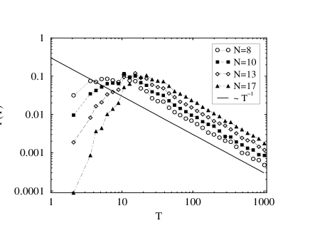
FIG. 1.: Distribution of evolution times for the local model. The data have been binned exponentially, hence the measured exponent is $\alpha-1$.

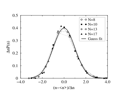
FIG. 2.: Distribution of the number of jumps for the local model, shifted and scaled by its mean and standard deviation.

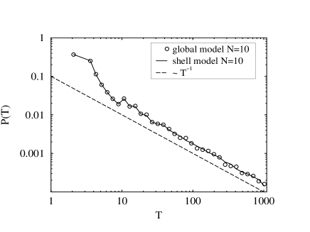
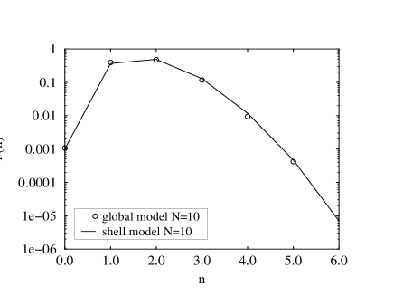
FIG. 3.: Comparison between the full global dynamics and the shell model for sequence length $N=10$. The number of realizations was $10^{6}$ for the full model and $10^{7}$ for the shell model. Upper panel: Binned distribution of evolution times. Lower panel: Distribution of the number of jumps.

REFERENCES

- [1] P. Bak and K. Sneppen, Phys. Rev. Lett. 71, 4083 (1993).
- [2] S.F. Elena, V.S. Cooper and R.E. Lenski, Science 272, 1802 (1996).
- [3] W. Fontana and P. Schuster, Science 280, 1451 (1998).
- [4] G.G. Simpson, Tempo and Mode in Evolution (New York, 1944).
- [5] For finite population effects see e.g. Y.C. Zhang, Phys. Rev. E 55, R3817 (1997); E. van Nimwegen and J.P. Crutchfield, Bull. Math. Biol. 62, 799 (2000).
- [6] W. Ebeling, A. Engel, B. Esser and R. Feistel, J. Stat. Phys. 37, 369 (1984).
- [7] Y.C. Zhang, Phys. Rev. Lett. 56, 2113 (1986).
- [8] C.M. Newman, J.E. Cohen and C. Kipnis, Nature 315, 400 (1985).
- [9] M. Eigen: Naturwissenschaften 58, 465 (1971)
- [10] M. Eigen, J. McCaskill, P. Schuster: Adv. Chem. Phys. 75, 149 (1989)
- [11] S. Galluccio: Phys. Rev. E 56, 4526 (1997)
- [12] J.S. McCaskill: Biol. Cybern. 50, 63 (1984); J. Chem. Phys. 80, 5194 (1984)
- [13] J. Krug, in Biological Evolution and Statistical Physics, ed. by M. Lässig and A. Valleriani (Springer, Berlin 2002).
- [14] J. Krug, T. Halpin-Healy: J. Phys. I France 3, 2179 (1993)
- [15] L. Peliti, cond-mat/9712027; S. Franz, L. Peliti, J. Phys. A 30, 4481 (1997)
- [16] C. Karl: Diploma thesis (University of Essen, 2001)
- [17] H.A. David, Order Statistics (Wiley, New York 1970)
- [18] P. Sibani, P.B. Littlewood: Phys. Rev. Lett. 71, 1482 (1993); P. Sibani, M. Brandt, P. Alstrøm: Int. J. Mod. Phys. B 12, 361 (1998)