Nonequilibrium dynamical mean-field theory of a strongly correlated system

Abstract

We present a generalized dynamical mean-field approach for the nonequilibrium physics of a strongly correlated system in the presence of a time-dependent external field. The Keldysh Green’s function formalism is used to study the nonequilibrium problem. We derive a closed set of self-consistency equations in the case of a driving field with frequency $\Omega$ and wave vector ${\bf q}$. We present numerical results for the local frequency-dependent Green’s function and the self-energy for different values of the field amplitude in the case of a uniform external field using the iterated perturbation theory. In addition, an expression for the frequency-dependent optical conductivity of the Hubbard model with a driving external field is derived.

The study of nonequilibrium many-body phenomena is a field of great and still growing interest in today’s condensed matter physics. Recent pump-probe experiments on transition metal oxides show unusual effects, e.g. a dramatic change in the optical transmission [1], which require a theoretical description of driven quantum systems. A basic model for theoretical investigations of strongly correlated fermion systems is the Hubbard model. Within the scope of the dynamical mean-field theory (DMFT) [2], a very detailed analysis of the spectral properties of the Hubbard model became possible. The DMFT approach takes into account local correlations as well as high energy excitations and provides a useful tool for calculating linear response functions of strongly correlated fermion systems [3, 4].

In this paper, we present a generalization of the DMFT using the Keldysh formalism to study a Hubbard model under the influence of a periodic external perturbation.

$$H = -\sum\limits_{\left<ij\right>\sigma}t_{ij}\left(c_{i\sigma}^{{\dagger}}c_{j\sigma}+c_{j\sigma}^{{\dagger}}c_{i\sigma}\right)+U\sum\limits_{i}n_{i\uparrow}n_{i\downarrow}$$ (2)

$$+\sum_{i\sigma}V_{i}(t)c_{i\sigma}^{{\dagger}}c_{i\sigma},$$

where $c_{i\sigma}^{{\dagger}}(c_{i\sigma})$ creates (annihilates) a fermion with spin $\sigma$ at site $i$ and $n_{i\sigma}=c_{i\sigma}^{{\dagger}}c_{i\sigma}$ is the local density operator. The bare half-filled single-band Hubbard model describes nearest-neighbor hoppings of electrons on a lattice, interacting with each other through the on-site Coulomb interaction. The additional explicitly time-dependent term in the Hamiltonian describes the external driving field with frequency $\Omega$, wave vector ${\bf q}=(q,...,q)$ and arbitrary field amplitude $A$.

$$V_{i}(t)=A\cos\left(\Omega t-{\bf qR}_{i}\right)$$ (3)

In particular we are interested in the small-$q$ limit. This Hamiltonian describes photodoping of a strongly correlated material, since the photon wavelength is large compared to the lattice spacing. For a uniform external field ($q=0$) the time-dependent perturbation term commutes with the Hubbard Hamiltonian, and this problem can be solved quite easily, as we will see later.

For large commensurate wave vectors, e.g. $q=\pi$, the $d$-dimensional lattice can be divided into cluster of $N=2\pi/q$ sites. The local properties depend on the chosen site ${\bf R}$ of this cluster. Performing the limit of a small wave vector is numerically limited by the increasing number of sites in the cluster. A theory which systematically includes nonlocal correlations to the DMFT is the dynamical cluster approximation (DCA) [5], where the original model is mapped onto a self-consistent embedded cluster instead of a single impurity.

The main technique for the treatment of nonequilibrium effects is the Keldysh Green’s function formalism [6, 7]. The usual time-ordering is replaced by a contour-ordering along the Keldysh contour, which follows the real-time axis from $-\infty$ to $+\infty$ and back to $-\infty$. The resulting Green’s functions matrix $G^{\alpha\beta}$, where $\alpha,\beta\in\{\pm 1\}$ specifies which time argument lies on the upper $(+)$, respectively lower $(-)$ branch of the Keldysh contour, defines three linearly independent components which provide information about the quantum states of the system (retarded/advanced Green’s function) as well as about their occupation out of equilibrium within a density matrix formulation (Keldysh component).

The external field is periodic in time and in each spatial coordinate. Thus, according to a generalized Floquet theorem [8], energy and momentum are conserved up to multiples of the external frequency and wave vector, respectively. We define a double Fourier transformation, expanding the Green’s function in its Floquet modes

$$G_{ij}^{\alpha\beta}(t,t^{\prime}) = \sum_{{\bf k},n}\int\frac{d\omega}{2\pi}e^{-i\omega t}e^{i\left(\omega-n\Omega\right)t^{\prime}}$$ (4)

$$\times e^{i{\bf kx}_{i}}e^{-i\left({\bf k}-n{\bf q}\right){\bf x}_{j}}G_{0n}^{\alpha\beta}\left({\bf k},\omega\right).$$ (5)

In the noninteracting case ($U=0$) and for small $q$, it is possible to calculate the Green’s function analytically by solving the equation of motion. The weighting coefficient of the $n$-th energy sideband turns out to be the Bessel function $J_{n}\left(A/\Omega_{q}({\bf k})\right)$ with $\Omega_{q}({\bf k})=\Omega-{\bf qv_{k}}$. Thus, the noninteracting retarded/advanced Green’s function is given by

$$g^{\mbox{ret/av}}_{0n}\left({\bf k},\omega\right) = \sum_{m}\frac{J_{m}(A_{q}({\bf k}))J_{m-n}(A_{q}({\bf k}))}{\omega-\epsilon_{{\bf k}}-m\Omega_{q}({\bf k})\pm i0^{+}}$$ (6)

where $A_{q}({\bf k})=A/\Omega_{q}({\bf k})$. The noninteracting Keldysh component reads

$$g^{\mbox{keld}}_{0n}\left({\bf k},\omega\right) = -2\pi i\sum_{m}\left(1-2f\left(\epsilon_{{\bf k}-m{\bf q}}\right)\right)$$ (10)

$$\times J_{m}(A_{q}({\bf k}))J_{m-n}(A_{q}({\bf k}))$$

$$\times\delta\left(\omega-\epsilon_{{\bf k}}-m\Omega_{q}({\bf k})\right).$$

The diagrammatic expansion of the Keldysh Green’s function matrix in the Coulomb parameter $U$ is mainly identical to Feynman theory [7]. The only difference arises from the summation over the two time branches.

We solve the driven Hubbard model using the dynamical mean-field approximation. Within DMFT the original lattice problem is mapped onto an effective impurity problem, which can be solved numerically, using e.g. quantum-Monte-Carlo simulations or iterated perturbation theory (IPT) [9, 10]. The local dynamics at a specific site ${\bf R}$ can be regarded as the interaction of the degrees of freedom at this site with an external bath created by all other degrees of freedom on other sites. Due to the spatial fluctuations for nonzero external wave vector the local properties depend on the chosen site ${\bf R}$ of the cluster.

The key approximation of the DMFT is the assumption of a local self-energy, which can be justified in the limit of large lattice connectivity [11, 12]. For the bare Hubbard model momentum conservation can be disregarded at each internal interaction vertex in the limit of infinite connectivity. An analogous argument for the driven Hubbard model yields that at internal vertices momentum conservation is automatically fulfilled up to multiples of ${\bf q}$. Thus, each internal propagator $G^{\alpha\beta}_{n_{1}n_{2}}({\bf k},\omega)=G^{\alpha\beta}_{{\bf k}-n_{1}{\bf q},{\bf k}-n_{2}{\bf q}}(\omega-n_{1}\Omega,\omega-n_{2}\Omega)$ can be replaced by $G^{\alpha\beta}_{0n}(\omega)=\sum_{\bf k}G^{\alpha\beta}_{q,0n}({\bf k},\omega)$ which is a “staggered” average over the lattice sites ${\bf R}$ in the cluster: $\sum_{{\bf R}}e^{-in{\bf qR}}G_{{\bf R}}(\omega)$. The resulting Dyson equation reads

$$G^{\alpha\beta}_{q,0n}\left(\omega\right) = g^{\alpha\beta}_{q,0n}\left(\omega\right)$$ (11)

$$+ \sum_{\gamma\delta,lm}\gamma\delta g^{\alpha\gamma}_{q,0l}\left(\omega\right)\Sigma^{\gamma\delta}_{q,lm}\left(\omega\right)G^{\delta\beta}_{q,mn}\left(\omega\right).$$ (12)

The mean-field description of the driven Hubbard model is determined by the effective Weiss field ${\cal{G}}_{\bf R}(t_{\alpha},t^{\prime}_{\beta})$, depending on the chosen site ${\bf R}$ of the cluster. The self-consistency condition is obtained by integrating out all degrees of freedom except those of the selected site ${\bf R}$. Assuming a semicircular bare density of states (Bethe lattice) one obtains the self-consistency condition for the Fourier transformed Weiss field, which is a matrix equation in energy and momentum sidebands and also in Keldysh space

$$\left[{\cal G}_{q}^{-1}\right]^{\alpha\beta}_{nm}(\omega) = \alpha\delta_{\alpha\beta}\bigg{[}\left(\omega-n\Omega\right)\delta_{nm}\bigg{.}$$ (16)

$$-\left.\frac{A}{2}\left(\delta_{nm+1}+\delta_{nm-1}\right)\right]$$

$$-\alpha\beta t^{2}\cos((n-m)q)G^{\alpha\beta}_{q,nm}(\omega).$$

We used the iterated perturbation theory (IPT) [9, 10] to solve the mean-field equations numerically for the half-filled driven Hubbard model. The basic idea of the IPT method is to perform a skeleton expansion of the self-energy up to second order in the interaction $U$:

$$\Sigma_{q,0n}^{\gamma\delta}(\omega) = \gamma\delta\ U^{2}\int\limits_{-\infty}^{\infty}\frac{d\omega_{1}}{2\pi}\int\limits_{-\infty}^{\infty}\frac{d\omega_{2}}{2\pi}\sum_{ml}{\cal G}_{q,l,0}^{\delta\gamma}\left(\omega_{1}\right)$$ (17)

$$\times {\cal G}_{q,0,n+m+l}^{\gamma\delta}\left(\omega_{1}+\omega_{2}\right){\cal G}_{q,0,-m}^{\gamma\delta}\left(\omega-\omega_{2}\right).$$ (18)

The matrix $G_{q,nm}$ is then obtained from the Dyson equation (11) with the noninteracting $g_{q,nm}$ replaced by the Weiss field ${\cal G}_{q,nm}$. The self-consistency loop is closed by calculating a new Weiss field from equation (16).

In our numerical calculation, we consider the special case of a uniform external field $(q=0)$, where the time-dependent perturbation term commutes with the bare Hubbard Hamiltonian and therefore the weighting coefficients of the energy sidebands are Bessel functions in the interacting case, too.

For $A=1$ and $A=2$ (we set $\Omega=1$), we restricted our considerations to the main energy band and the first three sidebands, i.e. we calculated the Fourier components $G_{0n}(\omega)$ with $n=-3,..,3$ (see Fig. 1). For $A=3$, we considered five sidebands: $n=-5,..,5$. These limitations of the number of sidebands are reasonable, since for a given $A$ the Bessel functions $J_{n}(A)$ fall off very fast with increasing $n$. This property strongly depends on the magnitude of the field: we have to take into account an increasing number of sidebands while enhancing the field amplitude.

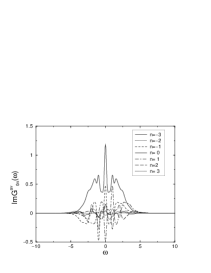
FIG. 1.: $\mbox{Im}G_{0n}^{\mbox{av}}(\omega)$ for $U=3$, $A=1$, three sidebands.

As an example, the Fourier components of the spectral density for $A=1$ are given in Fig. 1. From an inverse Fourier transformation of the advanced Green’s function, we obtained that the time-dependent advanced function satisfies the usual causality condition.

In the presence of the uniform external field, we define an effective spectral density, given by

$$\rho^{\mbox{eff}}(\epsilon)=\frac{1}{\pi}\mbox{Im}G_{00}^{\mbox{av}}(\omega)=\sum_{l}J_{l}^{2}(A)\frac{1}{\pi}\mbox{Im}\tilde{G}(\omega-l\Omega),$$ (19)

where $\tilde{G}$ is the local Green’s function for $A=0$. Fig. 2 shows how the effective spectral density depends on the field amplitude. In comparison with the usual three peak structure in the case of no external field (lower and upper Hubbard band and the quasiparticle peak), this function exhibits a more complex structure for $A\neq 0$ due to the sidebands, weighted by the Bessel functions. The number of occuring sidebands depends strongly on $A$: with increasing $A$, more sidebands become significant in the effective spectral density. An additional phenomenon is the strong suppression of the main quasiparticle peak for certain field amplitudes.

The effect of the external field on the imaginary part of the advanced self-energy on the field amplitude is shown in Fig. 3. For $A\neq 0$, we observe the sidebands of the typical two-peak structure in the equilibrium case.

FIG. 2.: $\mbox{Im}G_{00}^{\mbox{av}}(\omega)$ for $U=3$ and $A=0,1,2$, obtained by IPT.

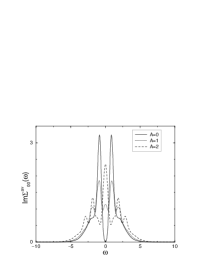
FIG. 3.: $\mbox{Im}\Sigma_{00}^{\mbox{av}}(\omega)$ for $U=3$ and $A=0,1,2$, obtained by IPT.

Finally, we consider the Keldysh component of the Green’s function, which contains information about the occupation of the states. From $G_{00}^{\mbox{keld}}$ we define an effective distribution function:

$$G^{\mbox{keld}}_{00}(\omega)=-2\pi i(1-2f^{\mbox{eff}}(\omega))\rho^{\mbox{eff}}(\omega)$$ (20)

For zero temperature and $A=0$, $f^{\mbox{eff}}$ is the usual Heaviside function. The effective distribution functions for $A=1,2,3$ are shown in Fig. 4. The modifications due to the external field at the energy sidebands of the Fermi edge correspond to emission and absorption processes of energy quanta $\Omega$. Experiments to measure the energy distribution function in a stationary out-of-equilibrium situation in metallic wires connected to two reservoir electrodes with an applied bias voltage have been done by Pothier et al. [13].

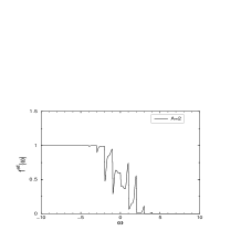
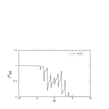
FIG. 4.: Effective distribution function for $A=0,1,2,3$ at $T=0$.

The time-dependent DMFT also provides a useful method for calculating the optical conductivity of the driven Hubbard model. Consider electrons described by the driven Hubbard model, which couple to an additional external classical vector potential with wave vector ${\bf p}$. Linear-response theory for nonequilibrium systems can be formulated quite simple in terms of Keldysh propagators. The paramagnetic current response in $\hat{\bf e}-$direction is given by

$$\left<J_{\hat{\bf e}}^{\mbox{param}}\left({\bf p},t\right)\right> = \frac{et}{2}\sum_{{\bf k}\sigma}v_{\hat{e}}\left({\bf k}+{\bf p},{\bf k}\right)G_{{\bf k}+{\bf p}{\bf k}\sigma}^{\mbox{keld}}(t,t)$$ (21)

with the vertex factor

$$v_{\hat{\bf e}}\left({\bf k}+{\bf p},{\bf k}\right)=e^{i({\bf k}+{\bf p})\hat{\bf e}}-e^{-i{\bf k}\hat{\bf e}}.$$ (22)

Just as in the case of the bare Hubbard Hamiltonian, all vertex corrections in the ladder decomposition of the current response function vanish in the limit of infinite dimensions [2, 3, 4, 14]. Thus, the optical conductivity is determined by the elementary particle-hole bubble as in the equilibrium case. Assuming isotropic spatial conditions, we obtain for the paramagnetic contribution

$$\sigma^{\mbox{param}}(\omega) = \frac{e^{2}}{2\omega d}\sum_{{\bf k}\sigma m}{\bf v}^{2}_{{\bf k}}\int\frac{d\omega^{\prime}}{2\pi}\left[G^{(0),\mbox{keld}}_{{\bf k}\sigma 0m}(\omega^{\prime}+\omega)\right.$$ (23)

$$\times \left.G^{(0),\mbox{av}}_{{\bf k}\sigma m0}(\omega^{\prime})+\ G^{(0),\mbox{ret}}_{{\bf k}\sigma 0m}(\omega^{\prime}+\omega)G^{(0),\mbox{keld}}_{{\bf k}\sigma m0}(\omega^{\prime})\right],$$ (25)

where $G^{(0)}$ denotes the zeroth order contribution in the classical vector potential, $\tau_{1}$ is the first Pauli matrix and ${\bf v_{k}}=\nabla_{\bf k}\epsilon_{\bf k}$. Using the spectral representation of the Green’s functions, the optical conductivity can be expressed in terms of the Fourier components of the spectral density $\rho^{l}_{0n}(\epsilon)=J_{l}(\frac{A}{\Omega})J_{l-n}(\frac{A}{\Omega})\mbox{Im}\tilde{G}^{\mbox{av}}(\epsilon-l\Omega)/\pi$ and the free density of states $D(\epsilon)$ (the diamagnetic term cancels the $1/\omega$-divergence of the paramagnetic part in the optical conductivity).

$$\sigma(\omega) = \frac{2\pi e^{2}t^{2}}{\omega}\sum_{l_{1},l_{2},m}\int\limits_{-\infty}^{\infty}d\epsilon\int\limits_{-\infty}^{\infty}d\omega^{\prime}D(\epsilon)$$ (29)

$$\times\quad\rho_{0m}^{l_{1}}(\epsilon,\omega^{\prime}+\omega)\rho_{m0}^{l_{2}}(\epsilon,\omega^{\prime})$$

$$\times\quad\left(f\left(\omega^{\prime}-l_{2}\Omega\right)-f\left(\omega^{\prime}+\omega-l_{1}\Omega\right)\right)$$

This final result for $\sigma(\omega)$ significantly shows the appearance of the energy sidebands due to the external driving field, and for zero driving field it reduces to the well-known expression for the optical conductivity of the bare Hubbard model.

We have generalized the DMFT equations using the Keldysh formalism to study a Hubbard model under the influence of a strong periodic external perturbation with arbitrary frequency and amplitude. We found that the Green’s functions were matrices in the energy and momentum sidebands due to quasi-energy and momentum conservation modulo the external frequency respectively wave vector.

We have derived a closed set of self-consistency equations for the driven Hubbard model wave vector numerically in the special case of a uniform field using IPT. We obtained an effective spectral density and distribution function for different values of the field amplitude. In addition, we have derived the frequency-dependent optical conductivity of the driven Hubbard model.

Solving the problem for a nonzero commensurate ${\bf q}$ would require an even larger numerical effort. One has to consider cluster of $N=2\pi/q$ sites and perform time-dependent DMFT for all sites ${\bf R}$ of this cluster. This is basically the same as using dynamical cluster approximation (DCA) [5] in combination with the Keldysh formalism. The original driven Hubbard model is mapped onto a self-consistent embedded cluster given by the periodic form of our Hamiltonian instead of a single impurity. Decreasing the wave vector requires solving cluster problems of increasing size, which is numerically limited because of an exponentially growing Hilbert space.

We are currently working on an application of the time-dependent DMFT to describe the local nonequilibrium physics of excitonic insulators and Mott insulators under laser excitation. This method shows great promise for being suitable to explain recent pump-probe experiments on transition metal oxides where unusual effects, e.g. a dramatic change in the optical transmission [1], have been observed. The real-time development of the DOS and the gap after the impact of a short intense laser pulse is under investigation.

REFERENCES

- [1] T. Ogasawara et al. Phys. Rev. Lett. 85, 2204 (2000)
- [2] A. Georges, G. Kotliar,, W. Krauth, M. J. Rozenberg, Rev. of Mod. Phys. 68, No 1, 13 (1996)
- [3] Th. Pruschke, D. L. Cox, M. Jarrell, Europhys. Lett. 21, No 5, 593 (1993)
- [4] Th. Pruschke, D. L. Cox, M. Jarrell, Phys. Rev. B 47, No 7, 3553 (1993)
- [5] M. H. Hettler et al. Phys. Rev. B 58, No. 12 (1998)
- [6] L. V. Keldysh Sov. Phys. JETP 20, No 4, 1018 (1965)
- [7] J. Rammer, H. Smith, Rev. of Mod. Phys. 58, No 2, 323 (1986)
- [8] P. Hänggi, Quantum transport and dissipation, Driven Quantum Systems, (1998)
- [9] A. Georges, G. Kotliar Phys. Rev. B 45, No 12, 6479, (1992)
- [10] E. Müller-Hartmann, Z. Phys. B 76, 211 (1989)
- [11] W. Metzner, D. Vollhardt, Phys. Rev. Lett. 62, No 3, 324 (1989)
- [12] E. Müller-Hartmann, Z. Phys. B 74, 506 (1989)
- [13] H. Pothier et al. Phys. Rev. Lett. 79, No. 18 (1997)
- [14] A. Khurana, Phys. Rev. Lett. 64, No. 16, 1990 (1990)