Adsorption of polyelectrolytes from semi-dilute solutions
on an oppositely charged surface

Abstract

We propose a detailed description of the structure of the layer formed by polyelectrolyte chains adsorbed onto an oppositely charged surface in the semi-dilute regime. We combine the mean-field Poisson-Boltzmann-Edwards theory and the scaling functional theory to describe the variations of the monomer concentration, the electrostatic potential, and the local grafting density with the distance to the surface. For long polymers, we find that the effective charge of the decorated surface (surface plus adsorbed polyelectrolytes) can be much larger than the bare charge of the surface at low salt concentration, thus providing an experimental route to a ”supercharging” type of effect.

I Introduction

When a charged solid surface (charge density $\sigma_{0}$) is exposed to a solution of polyelectrolytes carrying opposite ions ($Z$ charges per chain), a counter-ion exchange occurs such that the chains adsorb and the counter-ions initially retained captive by electrostatic attraction are released in the solution. This is because the system gains the translational entropy of the micro-ions, which is $Zk_{B}T$ (where $k_{B}T$ is the thermal energy), and only looses $k_{B}T$ for each adsorbed chain. Then at sufficiently high charge density, adsorbed polyelectrolytes form a dense layer of coils strongly bounded to the solid. In some favorable cases, because the macro-ions have very long tails dandling in the solution, the adsorbed layer alone may carry a surface charge density larger than $\sigma_{0}$. When the solution has been rinsed away, the decorated surface (solid surface plus attached chains) then behaves as a new charged system surrounded by counter-ions. This feature is the basic principle of a new device to build controlled charged multi-layers of alternated sign Decher .

On the theoretical side, the structure of the adsorbed layer is known in the dilute regime, where the chains in the bulk are isolated coils, and the solution does not affect much the layer Joanny ; DobryninDeshkovski ; Dobrynin ; Dobrynin2 ; varoqui ; stoll1 ; stoll2 . Comparatively, much less is known about adsorption from semi-dilute solutions. Because the dilute regime for polyelectrolytes is found at vanishing monomer concentrations ($\phi_{b}^{*}\sim N^{-2}$ where $N$ is the index of polymerization), the semi-dilute regime is certainly relevant from an experimental point of view. Note that the Decher process takes place in the semi-dilute regime in Ref. Decher2 . Borukhov et al. have numerically solved the non-linear mean-field system of equations in the semi-dilute regime for repulsive surfaces Borukhov . They also used scaling arguments to determine the relevant characteristic length scale in terms of the total electrostatic potential drop, but no detailed analytical description of the layer is done. Besides, the case of attractive surfaces does not simply follow from the repulsive case explicitly treated by Borukhov et al. since the concentration profiles are significantly affected by the boundary conditions. Châtellier and Joanny have solved the linearized mean-field system of equations suitable to describe how the charged surface affects the semi-dilute solution Chatellier . However, this approach is restricted to small perturbations. By solving numerically the self-consistent field equations using the ground state dominance approximation, Wang explored the influence of various parameters (surface charge, salt concentration, bulk concentration) on the occurrence of charge inversion wang . The latter was found to be strong at high salt concentration.

In any case, these works do not provide the extension, $H$, of the adsorbed layer (which does not identify with the characteristic relaxation length of the concentration), and the amount of material, $\Gamma$, attached to the solid surface (which does not identifies with the excess material driven to the interface $\int(\phi-\phi_{b})\,dz$, where $\phi$ is the monomer concentration, as defined in Refs. Borukhov ; Andelman ; wang ). There is a technical reason for that : the mean-field approach for adsorbed polyelectrolytes in semi-dilute conditions has to be supplemented by another approach to provide the full picture. This is because the variations of the polymeric concentration and the electrostatic potential does not carry enough information to completely describe the layer. This matters in practical situation since $\Gamma$ is directly related to the charge density carried by the decorated surface after removal from the solution. Accordingly, this quantity deserves a special attention. Moreover, it has been seen experimentally that the extension and the amount of material of the adsorbed layer vary significantly with $N$ Chibowski . This effect is not explained using the mean-field theory in the ground-state dominance approximation PGGbook alone, which is used in Refs. Borukhov ; Chatellier ; Andelman ; wang . Indeed within this approach, the semi-dilute solution is described with $\phi$ and the adsorbed chains cannot be distinguished from free chains in the semi-dilute layer.

In this article, we propose a complete description of the adsorbed layer in equilibrium with the semi-dilute solution. In particular, we estimate $\Gamma$ and $H$ as a function of $N$, $\sigma_{0}$ and $\phi_{b}$. We use a mean-field approach supplemented by a scaling type of description. The mean-field theory that we consider is the celebrated Poisson-Boltzmann-Edwards’ (PBE) description of the polyelectrolyte solution (see the reviews Andelman ; Barrat ). The scaling approach that we use is the Scaling Functional Theory (SFT) Manomacromol that we adapt to treat semi-dilute solutions of polyelectrolytes.

We shall consider a rather standard situation: long ($N\gg 1$), linear, fully flexible (the persistence length is identified with the monomer size $a$), polymer chains, small fraction of charges ($f\ll 1$), in $\Theta$ solvent conditions ($v=0$, and the monomer/monomer interaction is dominated by three body excluded volume interactions), bare surface charge $\sigma_{0}$. We assume no added salt and no specific interaction with the surface, as a first hint into the full problem. For definiteness, we suppose (without loss of generality) that the surface is negatively charged with a bare surface charge density $-\sigma_{0}$ (with $\sigma_{0}>0$), and the chain carries $Z=fN$ quenched elementary positive charges $+e$ where $f$ is the fraction of charged monomers.

In view of the number of parameters, this issue is a formidable task. To proceed further, our analysis is based on two major assumptions :
1. That we may find long polyelectrolyte tails belonging to adsorbed chains far from the surface (protruding in the solution), will be our first assumption (see Fig. 1). This hypothesis is inspired by the results found with long neutral chains adsorbed from semi-dilute solution, where we know that the concentration field decreases over a distance comparable to the bulk blob size $\xi_{b}\sim\phi_{b}^{-3/4}$ (the characteristic length scale of the solution), whereas the layer of adsorbed chains extend over much larger distances $H\cong R_{G}\sim N^{1/2}\phi_{b}^{7/8}$ Manomacromol ; Marques ; Daoud . In this example, the essential idea is that the collective response of the chains screens the perturbation induced by the surface at a characteristic length scale which does not depend on the chain size PGG81 . A similar feature is found with polyelectrolytes: in the semi-dilute regime, the Debye-Hückel length of the solution, $\kappa^{-1}$, is independent of the chain length. One may possibly argue that polyelectrolytes lie quite flat on the surface, as with dilute solutions. This is however very unlikely since for such picture extrapolated to very high concentrations of polyelectrolyte, it would mean that the adsorbed chains adopt an almost two-dimensional configuration. Clearly, the system of adsorbed chains would gain large amounts of conformational entropy by allowing more chains to adsorb and recovering an almost Gaussian structure (thus leaving some tails dandling in the solution), without perturbing much the distribution of charges in the vicinity of the solid. In other words, since $\kappa^{-1}\ll R_{G}\sim N^{1/2}$ in the limit $N\gg 1$, we expect that the influence of the surface will be small for the chain structure in equilibrium.
2. Looking at the variations of the electrostatic potential, $\Psi(z)$ with the distance to the surface, $z$, in the dilute regime, we anticipate a very simple form for $\Psi(z)$ in the semi-dilute regime (see Fig. 2). From the mean-field description of the layer in the dilute regime Joanny ; DobryninDeshkovski , we learn that the electrostatic potential first increases from negative values, then saturates, and eventually relaxes to zero. That there is a regime of parameters in the semi-dilute regime where such profile for $\Psi$ will persist to some extent be our second assumption. This assumption will be justified by the calculation but one can find a simple argument for it. The monomer concentration profile in the dilute regime tells us that the osmotic pressure decreases from the solid surface. Suppose that we increase the concentration of the solution from the dilute regime into the semi-dilute regime. Because the osmotic pressure close to the solid surface is much higher than what is found in the solution, we expect that the presence of the solution will affect the structure of the outer fringe of the layer, not the structure of the inner regions. Accordingly, we do not expect that the form of the electrostatic potential will be profoundly affected, at least in the semi-dilute regime close to the dilute regime.

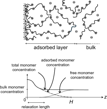
Figure 1: Sketch of the adsorbed polyelectrolyte layer exposed to a semi-dilute solution. Some long dandling tails and loops are protruding in the bulk. The total monomer concentration profile is thus the sum of the adsorbed monomer concentration and the free monomer concentration. We note that the relaxation length of the monomer concentration close to the surface is different from the total adsorbed layer thickness, $H$.

Following our second hypothesis, we define the plane of vanishing electrostatic field (such that $d\Psi/dz=0$) as the neutral plane. Similarly, we set the plane where the electrostatic potential vanishes (such that $\Psi\cong 0$) as the relaxation plane (we implicit assume that we haven chosen $\Psi(\infty)=0$). Then the layer might be divided into three main regions (labeled (1), (2) and (3), see Fig. 2) such that:

1. The compensation region stands between the solid surface and the neutral plane. By definition, the charges provided by the polyelectrolyte material situated in this region exactly compensate the surface charge.

2. The intermediate region stands between the neutral plane and the relaxation plane.

3. The outer region stands between the relaxation plane and the outer border of the layer, as defined by the longest polymeric coil in direct contact with the surface.

It is important to realize that this distinction, although a priori, is not arbitrary. Each of these region is well defined from a physical point of view.

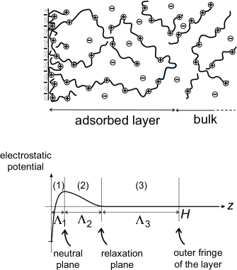
Figure 2: Sketch of the variations of the mean electrostatic potential in the direction perpendicular to the surface. It starts with a negative value at the negatively charged surface, increases until it reaches a maximum at the ”neutral plane”, where the electric field vanishes. Then it relaxes until it reaches its average value in the bulk, 0, at the relaxation plane and is constant in the outer region of the adsorbed layer.

In what follows, we first introduce the Scaling Functional Theory suitable to describe polyelectrolyte semi-dilute layers (Section 2). Then we propose a detailed picture for the adsorbed layer in Section 3. Section 4 presents our concluding remarks focusing on the issue of charge inversion. Scaling laws in polyelectrolyte solutions and the mean-field approach are briefly introduced in Appendices 1 and 2 respectively.

II Scaling functional theory

This theory was first introduced to describe neutral polydisperse polymeric layers by generalizing the Alexander-de Gennes model for brushes AGR . The basic principle is to describe the layer of adsorbed chains as a thermodynamical ensemble of tails and loops where the entropy associated with the polydispersity in size compete with the elastic energy and the monomer excluded volume. From a formal point of view, the SFT approach is a functional theory where the Hamiltonian is simplified according as follows ManoPRE : a) loops are cut into pseudo-tails, b) the tails and pseudo-tails are described by a single function $z$, where $z(n)$ is the position of the nth monomer, $n$, of each tail. This idea proved successful in describing various situation ranging from polymer brushes, reversible adsorption, irreversible adsorption, whatever the solvent conditions.

Our aim in this article is not to generalize the SFT to describe polyelectrolyte chains. Rather, we take advantage of the fact that in the semi-dilute regime, the chain is both Gaussian and neutral at large scales, and the system of polymers is thus analogous to a neutral solution provided that the blob is renormalized according to the physics at small scales. Essentially, our approach consists in integrating the degrees of freedom of the various species (including electrostatics interactions) into a proper description of the blob.

Within the SFT, the system of loops and tails attached to the solid surface is described by three functions: $S$, the local grafting density of tails and pseudo-tails (a function of the curvilinear distance $n$), $z$, the path, and $\phi$, the volume fraction of monomers. These functions are linked through the conservation of monomers:

$$\phi(z)=\frac{S(n(z))}{\dot{z}(n(z))}$$ (2.1)

For polyelectrolyte semi-dilute layers, the effective free-energy (per $cm^{2}$) of the system write ($\beta^{-1}=k_{B}T$):

$$\beta F\cong\int_{0}^{N}dn\left\{\frac{\left(a^{2}S(n)\right)^{3/2}}{\xi_{e}^{3/2}\dot{z}^{1/2}(n)}+a^{-1}\xi_{e}^{1/2}S^{3/2}(n)\dot{z}^{3/2}(n)-S^{\prime}(n)\ln\left(-\frac{S^{\prime}(n)}{S_{0}}\right)\right\}$$ (2.2)

where $S_{0}$ is the “grafting density” at the surface and $\xi_{e}\simeq a(f^{2}\ell_{B})^{-1/3}$ is the electrostatic blob size (in $\Theta$ solvent conditions, $\ell_{B}$ is the Bjerrum length in units of $a$, cf. Appendix 1). The effective free-energy eq. (2.2) is the sum of three contributions which account respectively for :
a) monomer excluded volume interactions. This contribution is $\int\Pi dz$, where the polymeric contribution to osmotic pressure, $\Pi$, scales as $k_{B}T/\xi^{3}$:

$$\Pi\cong k_{B}T\frac{\phi^{3/2}}{a^{3/2}\xi_{e}^{3/2}}$$ (2.3)

With eq. (2.1), it is simple to show that

$$\int_{0}^{H}\Pi dz\cong k_{B}T\int_{0}^{N}\frac{(a^{2}S(n))^{3/2}}{\xi_{e}^{3/2}\dot{z}^{1/2}(n)}\,dn$$ (2.4)

where $H=z(N)$ is the position of the last monomer and is identified as the layer thickness.
b) the elasticity of the tail at a scale larger than the blob size (after integration by parts)

$$\beta F_{el}=-\int_{0}^{N}dnS^{\prime}(n)\int_{0}^{n}\left(\frac{dz/\xi}{dm/g}\right)^{2}\frac{dm}{g}\cong a^{-1}\int_{0}^{N}\xi_{e}^{1/2}S^{3/2}(n)\dot{z}^{3/2}(n)dn$$ (2.5)

c) the entropy associated to the polydispersity in size of loops and tails which is similar for charged and neutral monomers as soon as polymers are flexible AGR .

Minimizing the free-energy eq. (2.2) with respect to $S$ and $\dot{z}$ yields two equations

$$\frac{3}{2}a^{3}\xi_{e}^{-3/2}\left(\frac{S}{\dot{z}}\right)^{1/2}+\frac{3}{2a}\xi_{e}^{1/2}S^{1/2}\dot{z}^{3/2}+\frac{S^{\prime\prime}}{S^{\prime}} = \mu_{b}$$ (2.6)

$$\frac{1}{2}\left(\frac{a}{\xi_{e}}\right)^{3/2}\left(\frac{S}{\dot{z}}\right)^{3/2}-\frac{3}{2a}\xi_{e}^{1/2}S^{3/2}\dot{z}^{1/2} = \Pi_{b}$$ (2.7)

These equations are formally similar to what we find in the neutral case (and their interpretation in physical terms is thus identical), except that the small scale structure introduces different scaling relationship. Equation (2.7) describes the local balance of forces (per unit surface parallel to the solid): elasticity (first term of lhs) competes with osmotic pressure (second term of lhs) and the bulk pressure (rhs). Note that the osmotic pressure of counter-ions is the same in the outer region and in the bulk so that it does not appear in eq. (2.7). Equation (2.6) describes the conservation of the generalized chemical potential. In equation (2.6), $\mu_{b}=\partial\Pi_{b}/\partial\phi_{b}$ is the chemical potential in the bulk and scales as $g_{b}^{-1}$:

$$\mu_{b}\cong\phi_{b}^{1/2}\left(\frac{a}{\xi_{e}}\right)^{3/2}$$ (2.8)

The bulk osmotic pressure, $\Pi_{b}\sim 1/\xi_{b}^{3}$, in equation (2.7) accounts for the pressure induced by the solution.

We emphasis that the SFT system of equations (2.6)–(2.7) assumes that the properties of the tails and loops are that of neutral strings of blobs, and may only apply to situations where the electrostatics interactions are screened at distances larger than the mesh size $\xi$ and especially very close to the substrate.

III Structure of the layer

III.1 Compensation region (1).

This region, close to the solid surface, is such that the charges provided by the polyelectrolyte material exactly compensate the surface charge. Hence

$$\Gamma_{1}\cong\sigma_{0}/f$$ (3.9)

and $\frac{d\Psi}{dz}\geq 0$ in this region (at the outer boundary of the compensation region: $\frac{d\Psi}{dz}=0$). For this reason, we expect that the counter-ions from polyelectrolytes are not present, $\rho^{-}\cong 0$. Moreover, at the low salt limit, positive counter-ions (from the charged surface) are negligible since their concentration is proportional to surface/volume and vanishes in the thermodynamic limit.

Each electrostatic blob carries $fg_{e}$ charges and occupies a surface $\xi_{e}^{2}$. These relation defines a critical value for $\sigma_{0}$ such that a single “carpet” of close packing electrostatic blob is able to fully compensate the surface charge:

$$\sigma_{c}\cong fa^{-2}$$ (3.10)

The monomer volume fraction inside this region is thus $\phi_{e}$, given by Eq. (0.41). Moreover, the electrostatic energy of a blob interacting with the surface is of order $k_{B}T$ for the critical value, $\sigma_{0}\simeq\sigma_{c}$, i.e. of the same order of the electrostatic repulsion between monomers. Accordingly, we shall distinguish two cases: $\sigma_{0}<\sigma_{c}$ and $\sigma_{0}>\sigma_{c}$ (Fig. 3).

III.A.1 Case $\sigma_{0}<\sigma_{c}$.

In this regime, we rely on the results found by Dobrynin et al. DobryninDeshkovski for the case of dilute solutions. The electrostatic attraction of charged monomers to the charged surface is weaker than the electrostatic repulsion between charged monomers. Therefore, the chain statistics is rod-like at scales larger than the blob $\xi$ (in the plane parallel to the surface) and Gaussian at smaller scales ($\xi\simeq ag^{1/2}$). However, the blob size is found by assuming that the electrostatic attraction to the surface is of order $k_{B}T$: $\frac{fg\sigma_{0}\xi^{2}e^{2}}{\epsilon\xi}\sim k_{B}T$ which leads to $\xi\simeq\xi_{e}\left(\frac{\sigma_{c}}{\sigma_{0}}\right)^{1/3}>\xi_{e}$. The chain segment is thus confined by the electrostatic attraction to the charged surface. However, contrary to the case of dilute solutions (single chain adsorption), polyelectrolytes do not lie flat on the surface since, as mentioned in the Introduction, the system gains conformational entropy by allowing more chains to adsorb with large loops protruding in the solution. The concentration of blobs in this region is found by assuming that this compensation layer actually compensates the surface charges and that the thickness is given by the confinement blob size $\xi$:

$$\Lambda_{1}\simeq\xi_{e}\left(\frac{\sigma_{c}}{\sigma_{0}}\right)^{1/3}$$ (3.11)

This scaling result has been shown numerically for semi-dilute solutions by Borukhov et al. Borukhov and Shafir et al. Shafir using the mean-field equations. The electric field vanishes at $z=\Lambda_{1}$ in this regime. Of course, we do not have a closed packing of these blobs, $\xi$, since the number of blobs per unit surface is $\sigma_{0}/fg\simeq(\sigma_{0}/\sigma_{c})^{5/3}\xi_{e}^{-2}<\xi_{e}^{-2}$.

This picture is valid only if the average monomer volume fraction close to the surface is higher than the bulk value, i.e. $\phi_{e}(\sigma_{0}/\sigma_{c})^{4/3}>\phi_{b}$ or

$$\sigma_{c}\left(\frac{\phi_{b}}{\phi_{e}}\right)^{3/4}\leq\sigma_{0}\leq\sigma_{c}$$ (3.12)

III.A.2 Case $\sigma_{0}>\sigma_{c}$.

In the limit $\sigma_{0}\gg\sigma_{c}$, the monomer volume fraction close to the surface, $\phi_{0}$, increases being larger than $\phi_{e}$, the electrostatic attraction becomes larger than the electrostatic intra-repulsion, and the osmotic pressure tends to swell the compensation region. Assuming that excluded volume interactions dominate over elasticity, as in Ref. DobryninDeshkovski , solving eq. (0.47) of Appendix 2 yields (at the leading order in $\phi_{e}/\phi_{0}\ll 1$ and assuming $\mu\simeq g_{e}^{-1}$ in this compensation region) a parabolic profile: $\phi(z)\cong\phi_{e}+(\phi_{0}-\phi_{e})(1-z/\Lambda_{1})^{2}$, where $\phi_{0}=(3\pi\ell_{B}\sigma_{0}^{2})^{1/3}$ and

$$\Lambda_{1}\cong\xi_{e}\left(\frac{\sigma_{0}}{\sigma_{c}}\right)^{1/3}$$ (3.13)

The structure of the compensation region is thus self-similar (see Fig. 3) as already described for the dilute case in Ref. DobryninDeshkovski . For the general case, the polymer elasticity is no more negligible and the full equation (0.47) must be solved without any approximation.

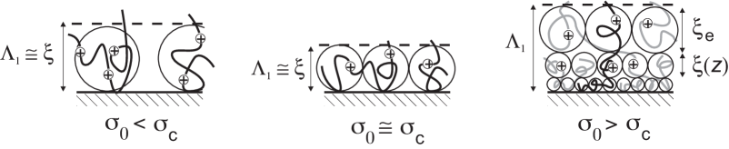
Figure 3: Sketch of the compensation region (1) in the 3 cases: $\sigma_{0}<\sigma_{c}$, $\sigma_{0}\simeq\sigma_{c}$ and $\sigma_{0}>\sigma_{c}$. The thickness of this region, $\Lambda_{1}$ decreases with $\sigma_{0}$ for $\sigma_{0}<\sigma_{c}$ and increases for $\sigma_{0}>\sigma_{c}$.

It is important to note that our result Eq. (3.13) is in contradiction with Andelman et al. Borukhov ; Andelman ; Shafir . They predict that the characteristic length scale of the adsorbed layer decreases with $\sigma_{0}$ (Andelman , eq. (71)) following Eq. (3.11). However, we argue that, for strong adsorption ($\sigma_{0}\gg\sigma_{c}$), the structure of the compensation region is found by balancing the electrostatic adsorption with the osmotic pressure (excluded volume interactions) and that chains are not confined. Instead of blobs of confinement, the structure is described in terms of osmotic blobs, in a similar way of describing neutral polymer layers.

Anyway, as we argue below (Section 4), in the semi-dilute regime and for long polyelectrolytes, we do not expect that this region has a dominant influence on observables such as the thickness of the layer, or the amount of material attached to the surface, and it is enough for our purpose to treat the restricted case where $\sigma_{0}\approx\sigma_{c}$, and

$$\Lambda_{1}\cong\xi_{e}$$ (3.14)

Anticipating the use of the SFT, it is useful to estimate the amount of monomers (per tail), $n_{1}$, involved in the compensation region. In a simple view where each tail contributes to one electrostatic blob, we find

$$n_{1}\cong g_{e}$$ (3.15)

and the local grafting density at the outer limit of the compensation region scales as

$$S(n_{1})\cong\frac{1}{\xi_{e}^{2}}$$ (3.16)

III.2 Intermediate region (2).

In this region, the direct electrostatic influence of the surface vanishes, and from this point of view, the structure should be similar to a layer of polyelectrolytes chains “adsorbed” onto a fictive neutral surface positioned at $z=\Lambda_{1}$. Here, the concentration of monomers decreases from $\phi_{e}$ to the bulk value, $\phi_{b}$. Because monomers and counter-ions are ruled by very different equations, the electrostatic potential $\Psi(z)$ does not vanish. As the system is globally neutral and $\phi(\Lambda_{1})=\phi_{e}>\phi_{b}$ in the semi-dilute regime, charge conservation in the system implies that the volume fraction of counter-ions, $\rho^{-}(z)$, will decrease from $\rho^{-}(\Lambda_{1})>f\phi_{b}$ to the bulk value $f\phi_{b}$ at the external border of region (2). Knowing that $\rho^{-}$ is related to the adimensional electrostatic potential $\Psi=\beta eV$ by $\rho^{-}=f\phi_{b}\exp\Psi$ (see Appendix 2), we deduce that $\Psi(\Lambda_{1})=\Psi_{1}$ is positive (with the boundary condition $\Psi(\infty)=0$). Thus, we expect that $\Psi(z)$ decreases monotonically from a finite positive value, $\Psi_{1}$ (to be estimated below), to 0.

When $\phi_{b}$ is not too small in comparison to $\phi_{e}$, say $\phi_{e}-\phi_{b}\ll\phi_{b}$, the linearized PBE system of equations described in Appendix 2 is justified to find the relaxation of the concentration profile. Note that for the case $\phi_{b}\ll\phi_{e}$ the full system should be solved numerically Borukhov ; Shafir . With the appropriate boundary conditions [$\phi(\Lambda_{1})=\phi_{e}$, $\phi(\infty)=\phi_{b}$, $d\Psi/dz(\Lambda_{1})=0$ and $\Psi(\infty)=0$], we find:

$$\varphi(z) = \sqrt{\phi_{b}}+\left(\sqrt{\phi_{e}}-\sqrt{\phi_{b}}\right)\left[(1-R)\,e^{-(z-\Lambda_{1})/\ell_{-}}+R\,e^{-(z-\Lambda_{1})/\ell_{+}}\right]$$ (3.17)

$$\Psi(z) = 8\pi\ell_{B}f\sqrt{\phi_{b}}\left(\sqrt{\phi_{e}}-\sqrt{\phi_{b}}\right)\left[\frac{1-R}{4\pi\ell_{B}f\phi_{b}-a^{2}\lambda_{-}}\right.$$ (3.18)

$$\times \left.\mathrm{e}^{-(z-\Lambda_{1})/\ell_{-}}+\frac{R}{4\pi\ell_{B}f\phi_{b}-a^{2}\lambda_{+}}\mathrm{e}^{-(z-\Lambda_{1})/\ell_{+}}\right]$$

$$\rho(z) = f\phi_{b}[\Psi(z)+1]$$ (3.19)

where

$$\ell_{\pm}^{-2} = \lambda_{\pm}=\frac{2\phi_{b}}{a^{2}}\left(\pi\ell_{B}f+6\phi_{b}\right)[1\pm\sqrt{\Delta}]$$ (3.20)

$$\Delta = 1-\frac{12\pi\ell_{B}f(2\phi_{b}^{2}+f)}{\phi_{b}(\pi\ell_{B}f+6\phi_{b})^{2}}$$ (3.21)

$$R^{-1} = 1-\sqrt{\frac{\lambda_{+}}{\lambda_{-}}}\frac{(4\pi\ell_{B}f\phi_{b}-a^{2}\lambda_{-})}{(4\pi\ell_{B}f\phi_{b}-a^{2}\lambda_{+})}$$ (3.22)

In Fig. 4 are plotted $\delta\varphi(z)=\varphi(z)-\sqrt{\phi}_{b}$ and $\Psi(z)$ for $\ell_{B}=1$, $f=0.1$, and $\phi_{b}=0.26$ (concentrated semi-dilute solution). Note that the characteristic relaxation lengths $\ell_{\pm}$ were obtained by Châtellier and Joanny Chatellier . In this reference, the possibility of damped oscillations in the volume fraction profile ($\ell_{\pm}$ imaginary) was carefully examined for lower values of $\phi_{b}$. Here, we will only consider the situation where $\ell_{\pm}$ are real numbers, for simplicity (the same discussion can be carried on with the real parts of $\ell_{\pm}$ in more general cases). Hence the surface induce an external perturbation to $\varphi$ of magnitude $\sqrt{\phi_{e}}-\sqrt{\phi_{b}}$ which relaxes, at the linear response level, to the bulk value, $\sqrt{\phi_{b}}$ on the characteristic wave length of the fluctuations in the bulk.

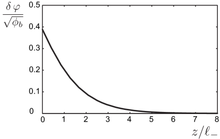
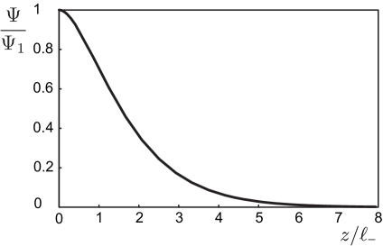
Figure 4: Polymer order parameter (left), $\delta\varphi/\sqrt{\phi}_{b}$, and electrostatic potential (right), $\Psi/\Psi_{1}$, as a function of the distance to $z=\Lambda_{1}$ (in units of $\ell_{-}$), in the intermediate region for $\ell_{B}=1$, $f=0.1$, and $\phi_{b}=0.26$, in the mean-field approximation.

Of course, we identify $\Lambda_{2}$ with the longest relaxation length, $\ell_{-}$:

$$\Lambda_{2}\cong\ell_{-}$$ (3.23)

It is instructive to compare the characteristic relaxation length $\ell_{-}$ with $\xi_{b}$, which requires that we simplify the expression given by eq. (3.20). Assuming that the intermediate region is dominated by the counter-ions pressure with an effective excluded volume $v_{\rm eff}\sim f/\phi_{b}$ (and that contribution arising from the monomers is negligible), the relaxation length $\ell_{-}$ writes (with $\Delta\simeq 1$):

$$\ell_{-}\approx\frac{a}{\sqrt{12\,f}}$$ (3.24)

In this limit, we have $\ell_{-}\leq\xi_{b}$ for $\phi_{b}\leq(f/\ell_{B})^{1/3}$, a reasonable case when $\phi_{b}<\phi_{e}$. The amount of monomers is this region is given by

$$\Gamma_{2}=a^{-3}\int_{\Lambda_{1}}^{\Lambda_{1}+\Lambda_{2}}\phi(z)dz\cong(0.17\phi_{b}+0.43\phi_{e}+0.40\sqrt{\phi_{b}\phi_{e}})\frac{\ell_{-}}{a^{3}}$$

Equation (3.18) also yields an estimate for the extremum value of the electrostatic potential $\Psi_{1}=\Psi(\Lambda_{1})$:

$$\Psi_{1}\cong 8\pi\ell_{B}f\sqrt{\phi_{b}}\left(\sqrt{\phi_{e}}-\sqrt{\phi_{b}}\right)\left[\frac{1-R}{4\pi\ell_{B}f\phi_{b}-a^{2}\lambda_{-}}+\frac{R}{(4\pi\ell_{B}f\phi_{b}-a^{2}\lambda_{+})}\right]$$ (3.25)

Equation (3.25) in turn allows to estimate $\Psi_{0}=\Psi(z=0)$ through the integrated Poisson equation:

$$\Psi_{0}=\Psi_{1}-4\pi\ell_{B}\sigma_{0}\Lambda_{1}+4\pi\ell_{B}f\int_{0}^{\Lambda_{1}}\int_{0}^{u}\phi(z)dzdu$$ (3.26)

For the moderate adsorption case ($\sigma_{0}\approx\sigma_{c}$) that we consider in this article, we find:

$$\Psi_{0}\cong\Psi_{1}-2\pi\ell_{B}\frac{fg_{e}}{\xi_{e}}$$ (3.27)

For the case of strong adsorption ($\sigma_{0}\gg\sigma_{c}$), we obtain:

$$\Psi_{0}\cong\Psi_{1}-2\pi\ell_{B}\frac{fg_{e}}{\xi_{e}}\left(\frac{\sigma_{0}}{\sigma_{c}}\right)^{4/3}$$ (3.28)

The SFT approach described in Section 2 is unlikely to describe correctly the intermediate region. At a simple scaling level, we will note that the local grafting density should drop from $S(n_{1})\cong\frac{1}{\xi_{e}^{2}}$ to $S(n_{2})\cong\frac{1}{\xi_{b}^{2}}$, where $n_{2}$ is the curvilinear index at $z=\Lambda_{1}+\Lambda_{2}$. A crude estimate for $n_{2}$ is found with a renormalized linear string approximation for the tails in the intermediate regime:

$$n_{2}\cong n_{1}+g_{e}\frac{\Lambda_{2}}{\xi_{e}}\simeq g_{b}$$ (3.29)

which is equivalent to write

$$\Lambda_{2}\cong\xi_{b}-\xi_{e}\simeq\xi_{b}$$ (3.30)

where the last approximation holds in the limit $\phi_{e}\ll\phi_{b}$. Hence, the thickness of region (2) is then given by equation (3.23) at a mean-field level and for $\phi_{e}-\phi_{b}\ll\phi_{b}$, and by equation (3.30) at a scaling level.

III.3 Outer region (3).

Here, the polymer concentration (resp. the counterion concentration, the adimensional electrostatic potential) is the bulk concentration, $\phi_{b}$ (resp. $f\phi_{b}$, 0 at scales larger than the bulk blob size), but the tails and loops in this region belong to chains in direct contact with the solid surface. At a scaling level of description, the layer is a close packing of semi-dilute blobs (size $\xi$). By analogy with the Rubinstein description of the bulk solution Rubinstein , we expect that electrostatic interactions are screened at distances larger than the mesh size $\xi$, and the system is amenable to a description in terms of neutral chains. Hence the SFT approach put forward in Section 2 is now appropriate.

Obviously, free and adsorbed chains interpenetrate, and we expect a slowly vanishing concentration profile for the monomers which belong to chains in direct contact with the surface, as depicted in Fig. 5a. In what follows, however, we assume that the free chains do not penetrate in the layer of tails and loops in direct contact with the surface. Accordingly, we consider a sharp, Heaviside type of profile at the outer fringe (see Fig. 5b). A similar type of simplification is found in various theories of polymeric layers. In the context of polymer brushes in good solvent, e. g., Alexander and de Gennes assume an Heaviside step for the concentration profile in order to find the extension of the layer Alexander ; PGGbrush . Their scaling result was confirmed by more refined theories where this constraint is relaxed (instead a parabolic profile is found) MWC . Similarly, Guiselin assumes no interpenetration in the context of molten solutions of neutral polymers adsorbed at an interface Guiselin . Here again, the scaling result was experimentally confirmed by measuring the amount of material irreversibly adsorbed Liliane . Because the semi-dilute solution is amenable to a description in terms of neutral blobs of strings of electrostatic coils PGGPincus ; Rubinstein , it is likely that the situation is analogous. In any case, we are confident that the scaling results that we find will not be dramatically affected by our simplification.

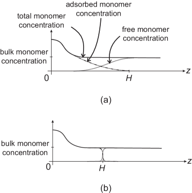
Figure 5: We expect a slowly vanishing concentration profile for the monomers which belong to chains in direct contact with the surface (a). In our approach, we simplify this picture into a sharp, Heaviside type of profile at the outer fringe (b).

The SFT equations suitable to describe this region are (2.6)–(2.7). In equilibrium, we expect that the bulk osmotic pressure exerted at the extremity of the layer ($z=H$) is balanced by the inner osmotic pressure, and the elasticity can be neglected in eq. (2.7). This yields

$$\frac{S}{\dot{z}}\cong\phi_{b}$$ (3.31)

and thus [eq. (2.1)], $\phi(z)\cong\phi_{b}$. When this relation is introduced into eq. (2.6), this equation simplifies into

$$\frac{\xi_{e}^{1/2}}{\phi_{b}^{3/2}}S^{2}+\frac{S^{\prime\prime}}{S^{\prime}}\cong 0$$ (3.32)

which admits a power law type of solution in the limit $N\rightarrow\infty$,

$$S(n)\cong\frac{\phi_{b}^{3/4}}{a^{2}(\xi_{e}/a)^{1/4}n^{1/2}}$$ (3.33)

Note that we find $S(n_{2})\cong\xi_{b}^{-2}$. Now solving Eqs. (3.31)–(3.33) (with the boundary condition $z(n_{2})\cong\Lambda_{1}+\Lambda_{2}$) for $z$, gives a Gaussian structure at large scale:

$$z(n)\cong\Lambda_{1}+\Lambda_{2}+a(\xi_{e}/a)^{-1/4}\phi_{b}^{-1/4}n^{1/2}$$ (3.34)

which readily yields [$H=z(N)$]:

$$\Lambda_{3}\cong a\frac{N^{1/2}}{(\xi_{e}/a)^{1/4}\phi_{b}^{1/4}}$$ (3.35)

and

$$\Gamma_{3}=\int_{n_{2}}^{N}S(n)\,dn\cong\frac{\phi_{b}^{3/4}N^{1/2}}{a^{2}(\xi_{e}/a)^{1/4}}$$ (3.36)

Note that the result eqs. (3.35)–(3.36) are precisely what we would find with scaling arguments assuming that the chains are Gaussian at large scale, and the SFT is only a formal way to recover them in this context. Figure 6 shows a scaling representation of the whole adsorbed layer in the case $\sigma_{0}\simeq\sigma_{c}$. On the other hand, $S$ is directly related to the loop size distribution $P$ through ManoPRE

$$S(n)=\int_{n}^{N}\,P(u)\,du$$ (3.37)

and eq. (3.33) may be experimentally checked with a surface force apparatus senden .

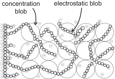
Figure 6: Scaling representation of the adsorbed layer of polyelectrolytes in the case $\sigma_{0}\simeq\sigma_{c}$ in terms of electrostatic blobs (size $\xi_{e}$) and concentration blobs (size $\xi_{b}$).

IV Discussion

The structure that we propose for the adsorbed layer clearly separates the influence of the charged surface which occurs only in the compensation region, from that of the bulk solution which act on the outer region, with an intermediate regime in between. We briefly describe the influence of $\phi_{b}$ and $\sigma_{0}$ on the layer structure and then discuss the occurrence of charge inversion for layers of very long charged chains.

We expect that as we increase $\phi_{b}$ from $\phi_{b}^{*}$, we progressively build the outer region at the expense of the intermediate region ($\Lambda_{2}$ decreases), but without much consequences for the compensation region. This is because the osmotic pressure of the counter-ions (the dominant contribution to the physics in the intermediate region) is much higher near $z=\Lambda_{1}$ than at $z=\Lambda_{2}$. Arguably, any increase of the bulk concentration of counter-ions will predominantly affect the low osmotic domain of the intermediate region, and hardly the structure near $z=\Lambda_{1}$, where the pressure is high. Of course, when $\phi_{b}$ reaches $\phi_{e}$, the intermediate region disappears in our simple view, and the bulk solution should then affect directly the compensation region. In this regime where fluctuations are negligible, numerical mean-field approaches are well adapted Borukhov ; wang . On the other hand, if we increase $\sigma_{0}$ from $\sigma_{c}$, at constant bulk concentration, the surface potential $|\Psi_{0}|$ increases and more and more monomers are involved in compensating the surface charge ($n_{1}$ and $\Lambda_{1}$ increase). Accordingly, the concentration profile in the compensating region is affected. But for very long chains ($N\gg n_{2}$), we do not expect that this should influence much the structure of the outer region.

Note that our description of the compensation and intermediate region resembles, but is not quite similar to the description of the adsorbed layer from dilute solution proposed in Ref. DobryninDeshkovski  : the so-called self-similar adsorbed layer regime. Essentially, we keep the parabolic decrease of the monomer volume fraction close to the surface, until we reach $\phi=\phi_{e}$ (where neglecting the chain elasticity is no more justified), and then we use the mean-field equations (which account for the elastic contribution and the osmotic pressure of counter-ions) to find the relaxation of $\phi$ below $\phi_{e}$. In Ref. DobryninDeshkovski , the region where $\phi\leq\phi_{e}$ is described in terms of electrostatic blobs. However such a description does not take into account the presence of the counter-ions in this region which is imposed by electroneutrality (the electric potential is positive). In technical terms, we make advantage of the fact that $\phi$ relaxes to a finite value, $\phi_{b}$, to determine the monomeric profile below $\phi_{e}$ by linearizing the mean-field equations. Because $\phi$ goes to $0$ in dilute solutions, such calculation is not possible and would necessitate a numerical resolution. The difference between the two descriptions is not just a matter of refinement since the relaxation of $\phi$ yields the variations of the electrostatic potential. With our approach, we provide both a coherent and complete picture for the variations of this quantity [eq. (3.18)].

A crucial aspect of adsorbed polyelectrolyte layers is their ability to capture a very large number of counter-ions per unit surface, much larger indeed than $\ell_{B}^{-2}$. In particular, the driving force for the adsorption of oppositely charged chains depends precisely on the amount of potentially free ions. With this in mind, it is interesting to discuss the following situation.

Suppose that we build an adsorbed layer from a semi-dilute solution, as described before. Then we remove the polymeric solution after the layer has equilibrated, but we suppose that the adsorbed chains remain attached to the charged surface, in a fashion similar to the scenario discussed by Guiselin for irreversible adsorption of molten liquids of neutral chains Guiselin . Finally, we put the decorated layer into a solution of pure solvent. The apparent charge (also called ”net charge” in Ref. DobryninDeshkovski ) of the layer in the dilute solution will be zero, because of the counter-ions present within (or in the proximity) of the layer. On the other hand, the decorated layer carries a huge amount per unit surface of potentially free counter-ions. Provided that we disregard the fluffy structure of the layer, the decorated surface effectively behaves as a new charged surface of ”nominal” charge density

$$\Delta\sigma\equiv\sigma-\sigma_{0} = f(\Gamma_{1}+\Gamma_{2}+\Gamma_{3})-\sigma$$ (4.38)

$$= f\Gamma_{2}+\ell_{B}^{1/12}f^{7/6}\phi_{b}^{3/4}N^{1/2}$$

Hence, for long chains, we expect that $\Delta\sigma$ may be much larger than $\sigma_{0}$.

Let us compare: a) a layer of polyelectrolytes reversibly adsorbed from dilute solution in equilibrium, and b) a layer of polyelectrolytes irreversibly adsorbed from semi-dilute solution put into a solution of pure solvent (the solid surfaces have the same $\sigma_{0}$ in both cases). To this aim, we need a precise vocabulary. We define three regimes, depending on the comparison of $\sigma$ with $\sigma_{0}$ and $2\sigma_{0}$:

• $\sigma<\sigma_{0}$: undercharging ($\sigma=\sigma_{0}$ corresponding to charge compensation);

• $\sigma_{0}<\sigma<2\sigma_{0}$: overcharging ($\sigma=2\sigma_{0}$ corresponding to charge inversion);

• $\sigma>2\sigma_{0}$: supercharging.

For case a) the mean-field theory predicts exact charge compensation in the absence of added salt Joanny . With added salt, Joanny finds overcharging, with possibly charge inversion in the limiting case of very high ionic force. In any case, there is no supercharging. It also appears that the surface controls the amount of adsorbed material in case a) (together with the ionic strength of the solution in case of added salt), not the chain length, nor the polymer concentration. A more recent analysis is provided by the work of Dobrynin et al. DobryninDeshkovski who carefully combine the mean-field theory with scaling arguments. But this study does not change the conclusions concerning the regime of compensation.

In contrast, for case b) our analysis strongly suggests that we have supercharging for sufficiently long chains, $N>(\sigma_{0}/f-\Gamma_{2})^{2}/[(\ell_{B}f^{2})^{1/6}\phi_{B}^{3/2}]$, even in the absence of salt.

V Concluding remarks

In this paper, we describe completely the structure of the adsorbed layer from semi-dilute solution by identifying the physical mechanisms in each sublayers : electrostatic attraction by the surface charge vs. three body interactions in the compensation region (1), importance of the polymer elasticity and the counter-ions osmotic pressure in the intermediate region (2), and presence of long tails and loops of adsorbed chains in the distal region (3) at the bulk concentration. We give explicit expressions for the coverage including all monomers belonging to adsorbed polymers, $\Gamma$ and the layer thickness $H$ as a function of parameters, bare surface charge, bulk concentration which could be checked experimentally.

Clearly, our description of the intermediate region suffers from several weaknesses. First, we consider a mean-field approach extrapolated outside its domain of validity. Secondly, we use a linearized theory, which is only justified for bulk volume fractions close to $\phi_{e}$. However, it is very likely that our essential scaling type of conclusions will be robust to any improved description of the intermediate region.

Similarly, the influence of the solvent quality (unless it is bad solvent) is rather limited. This is because the electrostatic interactions dominates over the excluded volume interactions at large scales, and in actual facts, the solvent only matters in the compensation region and in the electrostatic blob. For example, it is simple to show that $\Gamma_{3}\cong a^{-2}\phi_{b}^{3/4}(\ell_{B}f^{2})^{1/14}N^{1/2}$ and $\Lambda_{3}\cong a\phi_{b}^{-1/4}(\ell_{B}f^{2})^{1/14}N^{1/2}$ in good solvent conditions.

This study is limited to the very low salt limit. When the ionic force is very large, electrostatic interactions are screened at length scale larger than the Debye length and lead to an effective excluded volume $v_{el}=f^{2}/(2n_{s})$ where $n_{s}$ is the salt concentration Joanny ; Andelman . The structure of the compensation is then modified but far from the surface, the theory of neutral polymer layer Manomacromol can be applied by introducing the total excluded volume $v+v_{el}$ (where $v$ is the bare one). One find for instance $\Gamma_{3}\cong a^{-2}\phi_{b}^{7/8}[v+f^{2}/(2n_{s})]^{1/8}N^{1/2}$.

As far as we know, very few experimental measurements of the amount of material attached to the surface as a function of $N$ have been done under the conditions we are interested (oppositely charged surface, weakly charged chains, no salt added, semi-dilute solutions). The experiments of Chibowski et al. on adsorption of polyacrylic acid (PAA) and polyacrilamide (PAM) to a $\mathrm{Fe}_{2}\mathrm{O}_{3}$ solid surface, show a significant enhancement of both the layer thickness and the amount of material when the chain molecular weight is increased Chibowski . For instance, the thickness increases from 4.53 nm at molecular weight $M_{w}=$170 kg/mol to 6.69 nm at $M_{w}=$240 kg/mol for PAA at pH 3 and for a polymer concentration of 500 ppm (semi-dilute regime). This increase is in a qualitative agreement with Eq. (3.35) and is related to the formation of larger loops and tails. Of course, the authors mention the important role of the pH, since dissociation equilibriums are monitored by pH and thus both the number of charges of the chains and of the substrate can vary. Such effect has to be included in the theory to do a quantitative comparison.

Concerning the first step of the layer-by-layer process Decher , it should be pointed out that the adsorbed layer is globally neutral ($d\Psi/dz(H)=0$) because counter-ions which penetrate into the layer compensate the decorated surface charge. Hence it is not the apparent charge which is important but the amount of free counter-ions which can be released during the adsorption of oppositely charged polyelectrolytes. This is a key point since, by assuming that adsorbed chains stay upon rinsing, the driving force of adsorption is the exchange of counter-ions related to the amount of potentially free counter-ions. The good observable is thus the amount of adsorbed polymers $\Gamma$, and not the polymer surface excess relative to the bulk concentration. Hence the structure of the adsorbed layer, described in terms of loops and tails, is necessary to compute the coverage. We thus go beyond standard mean-field approaches Joanny ; varoqui ; stoll1 ; stoll2 ; Borukhov ; wang which cannot distinguish between adsorbed chains and free chains in the distal region. As a result, we find that the issue of overcharging–supercharging relies more on the chain length $N$ and bulk volume fraction $\phi_{b}$ than salt concentration : charge inversion occurs even at low salt concentration which underlines the role played by the chain length as a tunable experimental parameter. Presumably, this feature opens the way to a both simple and efficient way to tune the size of the successive layers in the Decher process. Obviously, a closer look at the case where two layers of oppositely charged polymers interpenetrate and rearrange ladam is required before we can drive any conclusion on the Decher process castel .

We are grateful to L. Bocquet, E. Trizac, G. Decher and R.R. Netz for interesting discussions.

Appendix 1 : scaling laws

In this Appendix, we briefly recall the basic scaling concepts for polyelectrolytes. We also provide the essential equations needed to understand the scaling arguments presented in the article. Our present understanding of weakly charged polyelectrolyte solutions without added salt is based on the concept of electrostatic blob PGGPincus ; Barrat : because the different charges of the backbone repel, the electrostatic interactions will deform the otherwise isotropic coil into an elongated string. At a scaling level, the chain is pictured as a linear string of electrostatic blobs (size $\xi_{e}$ , number of monomers $g_{e}$) such that $\beta\frac{\left(fg_{e}e\right)^{2}}{\epsilon\xi_{e}}\cong 1$. Let us assume $\Theta$ solvent conditions for simplicity (the two-body excluded volume parameter $v=0$). Then the Flory scaling law for random walks ($\xi_{e}\cong ag_{e}^{1/2}$) yields

$$\xi_{e}\cong\frac{a}{\left(f^{2}\ell_{B}\right)^{1/3}}\qquad\mathrm{and}\qquad g_{e}\cong\frac{1}{\left(f^{2}\ell_{B}\right)^{2/3}}$$ (0.39)

where $\ell_{B}=\frac{\beta e^{2}}{4\pi\epsilon a}$ is the Bjerrum length, in units of $a$. The extension of the polymer is

$$L\cong\frac{N}{g_{e}}\xi_{e}\cong aN\left(f^{2}\ell_{B}\right)^{1/3}$$ (0.40)

and the local volume fraction (inside the electrostatic blob),

$$\phi_{e}\cong\left(f^{2}\ell_{B}\right)^{1/3}$$ (0.41)

When the bulk concentration of monomers is larger than the overlapping concentration, $\phi_{b}^{*}\cong NL^{-3}\sim N^{-2}$, the widely accepted picture is that electrostatic interactions are screened at distances larger than the mesh size of the solution Rubinstein . Accordingly, the solution is a close packing of semi-dilute blobs (size $\xi_{b}$, number of monomers $g_{b}$, $\phi_{b}\cong g_{b}/\xi_{b}^{3}$), such that the chain is a Gaussian walk of blobs at a scale larger than $\xi_{b}$, and a linear string of electrostatic blobs at a scale smaller than $\xi_{b}$. We have PGGPincus

$$\xi_{b}\cong a\frac{\phi_{b}^{-1/2}}{\left(f^{2}\ell_{B}\right)^{1/6}}\qquad\mathrm{and}\qquad g_{b}\cong\frac{\phi_{b}^{-1/2}}{\left(f^{2}\ell_{B}\right)^{1/2}}$$ (0.42)

Eventually, when the bulk volume fraction exceeds $\phi_{e}$, the electrostatic blob vanishes, and the chain is Gaussian at all scales.

Appendix 2 : mean-field theory

In this Appendix, we recall the equations of the mean-field theory used to describe polyelectrolytes (see, e.g. Chatellier ; Andelman ). The basic idea is to describe the monomers as microscopic ions carrying a charge $fe$, with the following specific features: a) the translational entropy is negligible (this contribution scales as $(\phi/N)\log(\phi/N)$ and vanishes for long polymers ($N\gg 1$)), b) an excluded volume interaction estimated in mean-field, c) an elastic contribution to account for the chain deformation. Then the energy (per cm²) writes

$$\beta F = -\frac{1}{2a^{2}}\sigma_{0}\Psi(0)+\int_{0}^{\infty}\left[\Psi\rho^{+}-\Psi\rho^{-}-\frac{a^{2}}{8\pi\ell_{B}}(\nabla\Psi)^{2}\right]\frac{dz}{a^{3}}$$

$$+ \int_{0}^{\infty}\left[\rho^{+}(\ln\rho^{+}-1)+\rho^{-}(\ln\rho^{-}-1)\right]\frac{dz}{a^{3}}+\int_{0}^{\infty}\left[\frac{1}{3}\phi^{3}+\frac{a^{2}}{12}(\nabla\sqrt{\phi})^{2}+f\phi\Psi\right]\frac{dz}{a^{3}}$$

where the first term is the self-energy of the surface, the second term is the electrostatic energy of resp. the co-ions and the counter-ions and the self-energy of the electric field, the third term is the translational entropy of micro-ions (in volume fraction $\rho^{\pm}$), and the fourth term accounts for the energy of the monomers (resp.: three body-interaction with amplitude $w=a^{6}$, Edwards elastic contribution, electrostatic energy of the charged monomers). Minimizing the energy yields the Poisson-Boltzmann-Edwards (PBE) system of equations:

$$\frac{d^{2}\Psi}{dz^{2}}(z) = -\frac{4\pi\ell_{B}}{a^{2}}\left[f\phi(z)+n_{s}\mathrm{e}^{-\Psi(z)}-(n_{s}+f\phi_{b})\mathrm{e}^{\Psi(z)}\right]$$ (0.44)

$$\rho^{+}(z) = n_{s}\mathrm{e}^{-\Psi(z)}$$ (0.45)

$$\rho^{-}(z) = (n_{s}+f\phi_{b})\mathrm{e}^{\Psi(z)}$$ (0.46)

$$\frac{a^{2}}{6}\frac{1}{\sqrt{\phi(z)}}\frac{d^{2}\sqrt{\phi(z)}}{dz^{2}} = \phi(z)^{2}+f\Psi(z)-\mu$$ (0.47)

where $n_{s}$ is the volume fraction of salt in the bulk. Note that the mean-field theory is strictly valid for concentrations above $\phi_{e}$ for at least one reason: the average volume fraction, $\phi$, is not the local volume fraction experienced by the monomers, $\phi_{e}$, in the semi-dilute regime, and the three-body interactions (the term $\phi^{3}$ in eq. (Appendix 2 : mean-field theory)) is therefore incorrect. However, in the absence of any other theory to describe these systems, it is quite common to extrapolate the mean-field approach outside its strict domain of validity, and try to solve the PBE system of equation in the semi-dilute regime. Because $\mu$ is the chemical potential of the monomers in the solution, and this quantity is sensitive to the local concentration, it is tempting to correct for $\mu\cong 1/g_{e}$ ($\phi_{e}^{2}$ in theta solvent), while keeping the mean-field estimate of the chemical potential ($\phi(z)^{2}$ in our context) in the rhs of eq. (0.47). However, this approximation has a technical drawback since $\Psi(z)=0$, $\phi(z)=\phi_{b}$ is then not solution of the Edwards equation, as we expect far away from the surface. Here, we will keep the PBE system of equation with $\mu\cong\phi_{b}^{2}$. In Section 3.2, we use the Châtellier and Joanny approximation Chatellier where both the Boltzmann eq. (0.45–0.46) and Edwards eq. (0.47) are linearized (resp. around $\Psi=0$, and $\phi=\phi_{b}$). In terms of the polymer order parameter $\varphi=\sqrt{\phi}$, the PBE system of equation simplifies into

$$\frac{d^{2}\Psi}{dz^{2}}(z) = -\frac{8\pi\ell_{B}f}{a^{2}}\sqrt{\phi_{b}}\,\delta\varphi(z)+\left(\kappa^{2}+\frac{4\pi\ell_{B}}{a^{2}}\right)\Psi(z)$$ (0.48)

$$\rho^{+}(z) = n_{s}[1-\Psi(z)]$$ (0.49)

$$\rho^{-}(z) = \left(n_{s}+f\phi_{b}\right)[1+\Psi(z)]$$ (0.50)

$$\frac{a^{2}}{6\sqrt{\phi_{b}}}\frac{d^{2}\delta\varphi}{dz^{2}}(z) = 4\phi_{b}^{3/2}\delta\varphi(z)+f\Psi(z)$$ (0.51)

where $\Psi\ll 1$, $\varphi=\sqrt{\phi_{b}}+\delta\varphi$ (with $\delta\phi\ll\sqrt{\phi_{b}}$) and $\kappa^{2}=8\pi\ell_{B}n_{s}/a^{2}$.

References

- (1) G. Decher, Science, 1997, 277, 1232.
- (2) J.-F. Joanny, Eur. Phys. J. B, 1999, 9, 117.
- (3) A. V. Dobrynin, A. Deshkovski, M. Rubinstein Phys. Rev. Lett., 2000, 84, 3101.
- (4) A. V. Dobrynin, J. Chem. Phys., 2001, 114, 8145.
- (5) A. V. Dobrynin, M. Rubinstein, J. Phys. Chem. B, 2003, 107, 8260.
- (6) R. Varoqui, J. Phys. II France, 1993, 3, 1097.
- (7) P. Chodanowski, S. Stoll, Macromolecules, 2001, 34, 2320.
- (8) A. Laguecir, S. Stoll, Polymer, 2005, 46, 1359.
- (9) M. Lösche, J. Schmitt, G. Decher, W. G. Bouwman, K. Kjaer, 1998, Macromolecules, 31, 8893.
- (10) I. Borukhov, D. Andelman, H. Orland, Macromolecules, 1998, 31, 1665.
- (11) X. Châtellier, J.-F. Joanny, J. Phys. II France, 1996, 6, 1669.
- (12) Q. Wang, Macromolecules, 2005, 38, 8911.
- (13) R. R. Netz, D. Andelman, Polyelectrolytes in solution and at surfaces In M. Urbackh and E. Giladi editors, Encyclopedia of Electrochemistry (Wiley-VCH, Weinheim, 2002).
- (14) S. Chibowski, M. Wiśniewska, Colloids Surf. A, 2002, 208, 131.
- (15) P.-G. de Gennes, Scaling Concepts in Polymer Physics, 2nd ed. (Cornell University Press, Ithaca and London, 1985).
- (16) J.-L. Barrat, J.-F. Joanny, Adv. Chem. Phys., 1996, 94, 1.
- (17) M. Manghi, M. Aubouy, Macromolecules, 2000, 36, 5721.
- (18) C. M. Marques, J.-F. Joanny, J. Phys. France, 1988, 49, 1103.
- (19) M. Daoud, G. Jannink, J. Phys. II France, 1991, 1, 1483.
- (20) P.-G. de Gennes, Macromolecules, 1981, 14, 1637.
- (21) M. Aubouy, O. Guiselin, E. Raphaël, Macromolecules, 1996, 29, 7261.
- (22) M. Manghi, M. Aubouy, Phys. Rev. E, 2003, 68, 041802.
- (23) A. Shafir, D. Andelman, R.R. Netz, J. Chem. Phys., 2003, 119, 2355.
- (24) A. V. Dobrynin, R. H. Colby, M. Rubinstein, Macromolecules, 1995, 28, 1859.
- (25) S. Alexander, J. Phys. France, 1977, 38, 983.
- (26) P.-G. de Gennes, Macromolecules, 1980, 13, 1069.
- (27) S.T. Milner, T.A. Witten, M.E. Cates, Europhys. Lett., 1988, 5, 413.
- (28) O. Guiselin, Europhys. Lett., 1992, 17, 225.
- (29) L. Léger, E. Raphaël, H. Hervet, Adv. Polymer Sci., 1999, 138, 185.
- (30) P.-G. de Gennes, P. Pincus, R. M. Velasco, F. Brochard, J. Phys. France, 1976, 37, 1461.
- (31) T. Senden, J.-M. Di Meglio, P. Auroy, Eur. Phys. J. B, 1998, 3, 221.
- (32) G. Ladam, P. Schaad, J.C. Voegel, P. Schaaf G. Decher, F. Cuisinier, Langmuir, 2000, 16, 1249.
- (33) M. Castelnovo, J.-F. Joanny, Langmuir, 2000, 16, 7524.