The osmotic pressure of charged colloidal suspensions:
A unified approach to linearized Poisson-Boltzmann theory

Abstract

We study theoretically the osmotic pressure of a suspension of charged objects ($e.\,g.$, colloids, polyelectrolytes, clay platelets, etc.) dialyzed against an electrolyte solution using the cell model and linear Poisson-Boltzmann (PB) theory. From the volume derivative of the grand potential functional of linear theory we obtain two novel expressions for the osmotic pressure in terms of the potential- or ion-profiles, neither of which coincides with the expression known from nonlinear PB theory, namely, the density of microions at the cell boundary. We show that the range of validity of linearization depends strongly on the linearization point and proof that expansion about the selfconsistently determined average potential is optimal in several respects. For instance, screening inside the suspension is automatically described by the actual ionic strength, resulting in the correct asymptotics at high colloid concentration. Together with the analytical solution of the linear PB equation for cell models of arbitrary dimension and electrolyte composition explicit and very general formulas for the osmotic pressure ensue. A comparison with nonlinear PB theory is provided. Our analysis also shows that whether or not linear theory predicts a phase separation depends crucially on the precise definition of the pressure, showing that an improper choice could predict an artificial phase separation in systems as important as DNA in physiological salt solution.

I Introduction

In this paper we study the osmotic pressure of a suspension of charged colloids or polyelectrolytes in osmotic equilibrium with an electrolyte of given composition. Examples of such systems abound in our everyday life. They occur as dispersion paints, viscosity modifiers, flocculants, or superabsorbers, to name but a few technological applications Hun94 ; DaJa94 . They also play a tremendous role in molecular biology, since virtually all proteins in every living cell, as well as the DNA molecule itself, are charged macromolecules dissolved in salty water LoBe01 . A great deal of experimental and theoretical research has been devoted to their understanding, and several good textbooks Hun94 ; DaJa94 ; Oos71 ; RuSa89 ; EvWe99 ; Rad01 and review articles Kat71 ; BaJo96 ; HaLo00 ; Bel00 are available.

Arguably the most fundamental thing to know about these suspensions is their equation of state, $i.\,e.$, how the (osmotic) pressure depends on other thermodynamic variables like macromolecular charge or concentration. Within the last hundred years several ingenious ways have been conceived for treating this problem on varying levels of sophistication. In this article we will be concerned with Poisson-Boltzmann (PB) theory in combination with a cell model approximation for the macroion correlations, which we briefly revisit in Sec. II. While this does not present the highest level of accuracy or sophistication, it is probably the simplest and up to today single most important starting point; it offers a benchmark against which all other theories are compared. Indeed, we believe that modern improvements can only be fully appreciated once one understands the successes and failures of the most fundamental mean field theories.

Since the nonlinear PB equation can be solved analytically only in very few cases And95 , its linearized version has always been an important substitute. However, the freedom to choose an expansion point and its subsequent impact on the range of validity and accuracy of the linearization has often gone unnoticed. Moreover, the computation of thermodynamic properties from the ionic profiles computed in linear theory is often based on expressions from the nonlinear PB theory or expansions thereof PaGi72 ; RuBe81 ; StRi87 ; HaPo01 . This procedure is by no means unique and invariably entails internal inconsistencies. Both these points make it virtually impossible to conclude whether any failures of linearized PB theory are real deficiencies or avoidable side-effects of a non-optimal or inconsistent linearization.

In this paper we resolve these issues by giving a coherent presentation of linearized PB theory which illuminates the subtle interrelations between the Donnan equilibrium, microion screening, linearization and the osmotic pressure. In Sec. III we utilize the functional approach to PB theory Lev39 ; BrRo73 ; ReRa90 and generalize its quadratic expansion LoHa93 , arriving at a functional which yields the PB equation linearized about the electrostatic potential value $\bar{\psi}$. This expansion point will turn out to lie at the heart of all those interrelations. For general $\bar{\psi}$ we then derive in Sec. IV an analytical formula for the pressure in terms of the ionic profiles. Our novel expression replaces the famous boundary density rule Mar55 from nonlinear PB theory, according to which the osmotic pressure of the suspension is given by the value of the microion density at the outer cell boundary. That this does not hold in linearized theory may be considered as one of the major results of the present work.

The most common choice of the linearization point $\bar{\psi}$ – namely, the potential value in the salt reservoir – suffers from several drawbacks, as this value can be very different from the average electrostatic potential $\langle\psi({\boldsymbol{r}})\rangle$ in the colloidal suspension, and it seems more reasonable to selfconsistently linearize about the latter RuBe81 ; TrHa96 ; TrHa97 ; GrRo01 . We investigate this choice in Sec. V and will prove that it is indeed optimal—in the sense that ($i$) charge screening rests on the actual ionic strength, such that ($ii$) the crossover between counterion- and salt-screening is naturally included and ($iii$) the limit of large volume fraction is correctly reproduced. In brief, all zeroth order effects of the Donnan-equilibrium are already incorporated by the mere choice of the linearization point, and the linearized equation now describes higher order effects. We will also see that ($iv$) all other choices of the linearization point overestimate the Donnan effect in lowest order, since they violate a rigorous inequality from PB theory for the salt content in the colloidal suspension.

Based on this optimal linearization scheme we then derive explicit analytical formulas for the osmotic pressure of suspensions of charged mesoscopic objects in Sec. VI. These formulas hold for spherical, cylindrical and planar shapes and should thus be useful in a broad variety of possible systems. The subsequent Section VII is devoted to comparing their predictions with the full nonlinear PB theory.

Within full PB theory the pressure is always positive. Whether or not this also holds in the linearized theory depends both on the choice of the linearization point $\bar{\psi}$ as well as on the precise definition of the pressure itself. We prove that the pressure is always positive for symmetric electrolytes if one treats $\bar{\psi}$ as an independent variable. If one does not, the pressure can become negative at low volume fractions GrRo01 ; RoHa97 ; CaTr98 ; RoDi99 ; War00 ; DiBa01 . The implied liquid-gas coexistence – not being present on the nonlinear level – is thus clearly an artifact. As a striking example we show that even a solution of DNA molecules under physiological conditions would be predicted to phase separate at all relevant densities.

II General framework

In this section we start by introducing the physical situation we wish to describe – namely, the Donnan equilibrium – and its theoretical description in terms of a cell model. PB theory is founded on its grand potential functional, and a brief derivation for the pressure (leading to the boundary density rule) is presented.

II.1 The Donnan equilibrium

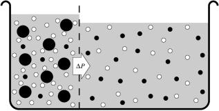
Figure 1: A solution of charged objects is in osmotic (Donnan-) equilibrium with a salt reservoir of given composition. The membrane is permeable for small ions only and has to support an excess osmotic pressure $\Delta P$. The mesoscopic objects are depicted as spherical (as appropriate for instance for “conventional” charged colloids or micelles), but our discussion will be more general and also apply to cylindrical entities ($e.\,g.$ DNA, actin filaments, TMV viruses) or planar objects ($e.\,g.$ charged membranes, clay particles).

We study a suspension of charged mesoscopic objects (henceforth simply referred to as “colloids”) dialyzed against a salt reservoir of given composition, as illustrated in Fig. 1. This situation is traditionally referred to as a “Donnan membrane equilibrium” Don24 ; Ove56 ; TaLe98 . Much of our discussion will not depend on the shape of the colloids, and our final explicit formulas will be valid for spherical, cylindrical and planar geometries. Even though the microions can traverse the membrane, their average concentration differs between the salt reservoir and the colloid compartment, since the latter is already occupied by the counterions originating from the macroions, which cannot leave the compartment due to the constraint of global electroneutrality. This imbalance in average densities generates an osmotic pressure difference which the membrane has to sustain and which we wish to calculate in the following.

For simplicity we assume the reservoir to be sufficiently large such that its ionic strength remains unchanged after being brought in contact with the macroion solution. This assumption is not necessary, but simplifies our discussion of general theoretical issues. How it can be avoided is demonstrated in Ref. TaLe98 . We also note that we will not describe the solvent explicitly but rather replace it by a continuum with relative dielectric constant $\varepsilon_{\operatorname{r}}$.

II.2 Cell-model and Poisson-Boltzmann theory

Theoretical concepts like the cell-model or PB theory have long become standard tools, so we will restrict ourselves to a brief description and only provide the basic equations—essentially in order to introduce our notation and terminology. A recent and more detailed exposition can be found in Ref.  DeHo01 .

The cell model approximation attempts to reduce the complicated many particle problem of interacting charged colloids and microions to an effective one-colloid-problem. It rests on the observation that at not too low volume fractions the colloids – due to mutual repulsion – arrange their positions such that each colloid has a region around it which is void from other colloids and which looks rather similar for different colloids. In other words, the Wigner-Seitz cells around two colloids are comparable in shape and volume. One now assumes that ($i$) the total charge within each cell is exactly zero, ($ii$) all cells have the same shape and ($iii$) for actual calculations one may approximate this shape such that it matches the symmetry of the colloid (for instance, spherical cells around spherical colloids). If the radius of the colloids is $r_{0}$, the cell radius $R$ is chosen such that $\phi=(r_{0}/R)^{d}$ equals the volume fraction occupied by the colloids. Here, $d$ measures the “dimensionality” of the colloid in the sense that $d=1$, $2$ and $3$ corresponds to planar, cylindrical and spherical colloids. If one ($iv$) neglects interactions between different cells, the partition function finally factorizes in the macroion coordinates, $i.\,e.$, the thermodynamic potential of the whole suspension is equal to the number of cells times the thermodynamic potential of one cell.

Within each cell the small ions assume some inhomogeneous distribution which arises from their interactions with themselves as well as with the charged colloid. Computing the corresponding partition function is impracticable, since all ions are strongly correlated with each other. Poisson-Boltzmann theory is the mean-field route to circumventing precisely this problem. A very powerful way to formulate it starts from a thermodynamic potential functional belonging to the appropriate ensemble—which in our case is the grand canonical one:

$$\beta\Omega = \int_{V}{\operatorname{d}}^{d}r\;\bigg{\{}\frac{1}{2}\psi({\boldsymbol{r}})\Big{(}\rho_{\operatorname{f}}({\boldsymbol{r}})+\sum_{i}v_{i}\,n_{i}({\boldsymbol{r}})\Big{)}$$ (1)

$$\qquad\qquad+\sum_{i}n_{i}({\boldsymbol{r}})\Big{(}\log\big{(}n_{i}({\boldsymbol{r}})\Lambda^{d}\big{)}-1\Big{)}$$

$$\qquad\qquad-\sum_{i}\mu_{i}\,n_{i}({\boldsymbol{r}})\bigg{\}}.$$

The meaning of the symbols is as follows: $\beta\equiv 1/k_{\operatorname{B}}T$ is the inverse thermal energy; $\psi({\boldsymbol{r}})$ is the local electrostatic potential (made dimensionless by multiplication with $\beta e$, where $e$ is the positive unit charge); the potential is generated by both the fixed charge density $e\rho_{\operatorname{f}}({\boldsymbol{r}})$ (located for instance on the colloid surface) as well as the distributions $n_{i}({\boldsymbol{r}})$ of mobile ions of species $i$, which have a signed valence $v_{i}$ and a chemical potential $\mu_{i}$; $\Lambda$ is the thermal de Broglie wavelength of the small ions; and the region of integration, $V$, is understood to be the space within one cell that is actually accessible to the small ions. The functional minimization of (1) subject to the constraint of Poisson’s equation and charge conservation yields the set of Euler-Lagrange equations

$$n_{i}({\boldsymbol{r}})\;=\;\Lambda^{-d}\,{\operatorname{e}}^{\mu_{i}}\,{\operatorname{e}}^{-v_{i}\psi({\boldsymbol{r}})}\;=\;n_{i,{\operatorname{b}}}\,{\operatorname{e}}^{-v_{i}\psi({\boldsymbol{r}})}.$$ (2)

The $n_{i,{\operatorname{b}}}$ are the concentrations of ions of species $i$ in the salt reservoir where the electrostatic potential has been assumed to vanish. Combining Eqn. (2) with Poisson’s equation results in the nonlinear Poisson-Boltzmann differential equation for the potential $\psi({\boldsymbol{r}})$ in the region within the cell accessible to the microions. After introducing the Bjerrum length $\ell_{\operatorname{B}}:=\beta e^{2}/\varepsilon_{\operatorname{r}}$, it is written as

$$\Delta\psi({\boldsymbol{r}}) = -4\pi\,\ell_{\operatorname{B}}\sum_{i}v_{i}\,n_{i}({\boldsymbol{r}})$$ (3)

$$\stackrel{{\scriptstyle\text{(\ref{eq:Boltzmann})}}}{{=}} -\kappa^{2}\,\frac{\sum_{i}v_{i}\,n_{i,{\operatorname{b}}}\,{\operatorname{e}}^{-v_{i}\psi({\boldsymbol{r}})}}{\sum_{i}v_{i}^{2}\,n_{i,{\operatorname{b}}}},$$

with the Debye screening constant of the reservoir defined as

$$\kappa^{2}\;:=\;4\pi\ell_{\operatorname{B}}\sum_{i}v_{i}^{2}\,n_{i,{\operatorname{b}}}.$$ (4)

If we reinsert the solution of this equation back into the functional (1) and use Eqn. (2), we obtain its equilibrium (=minimum) value, which is the grand potential of nonlinear PB theory:

$$\beta\Omega_{\operatorname{eq}} = \frac{1}{2}\int_{V}{\operatorname{d}}^{d}r\;\rho_{\operatorname{f}}({\boldsymbol{r}})\psi({\boldsymbol{r}})$$ (5)

$$-\int_{V}{\operatorname{d}}^{d}r\;\sum_{i}n_{i}({\boldsymbol{r}})\Big{[}1+\frac{1}{2}v_{i}\,\psi({\boldsymbol{r}})\Big{]}.$$

We want to close with the following remarks: The above variational principle can be constructed starting from the PB equation (see for instance Ref. ReRa90 and references therein), but this need not give a unique functional FoBr97 and (once $\Omega$ has been identified with the grand potential) appears like an upside-down explanation for the key initial equation (2). However, PB theory can be well justified by deriving the functional (1) from the underlying Hamiltonian. For instance, it can be obtained as the saddle point of the field theoretic action PoZe88 ; CoDu92 ; NeOr00 ; BoAn00 , as a density functional reformulation of the partition function combined with a first order cumulant expansion of the correlation term LoHa93 , or from the Gibbs-Bogoljubov inequality applied to a trial product state DeHo01 . Those approaches also show that PB theory provides an upper bound of the exact thermodynamic potential.

II.3 The pressure in Poisson-Boltzmann theory

One advantage of the thermodynamic functional approach to PB theory is that it becomes immediately clear what the pressure is—in the present ensemble the derivative of the grand potential (5) with respect to the volume. It proves convenient to rewrite this in terms of the functional (1), which can be achieved as follows. The variation upon some change in volume can be decomposed into the “orthogonal” changes

$$\delta\Omega\;=\;\frac{\partial\Omega}{\partial V}\bigg{|}_{n_{i}({\boldsymbol{r}})}\!\!\!\!\delta V+\int_{V}{\operatorname{d}}^{d}r\sum_{i}\frac{\delta\Omega}{\delta n_{i}({\boldsymbol{r}})}\bigg{|}_{V}\delta n_{i}({\boldsymbol{r}}),$$ (6)

where the first term contains any explicit dependence on the volume (at fixed ion profiles) and the second part is the implicit dependence through the ion profiles (at fixed volume). However, since the equilibrium distributions make the grand potential functional stationary with respect to variations of the density profile at fixed cell geometry, the implicit terms vanish. Hence, the pressure is just the negative derivative of the grand potential functional with respect to the cell volume, evaluated at the equilibrium profile. The derivative $\partial/\partial V$ is understood to imply a movement of the outer neutral cell boundary, which shall be located at $r=R$, and which only occurs in the boundaries of the volume integral in Eqn. (1). Note that rewriting the electrostatic energy in terms of the densities gives a double integral, and the product rule then cancels the prefactor $1/2$ in front of the term describing the electrostatic energy. Putting everything together, one arrives at

$$\beta P = -\frac{\partial\,\beta\Omega_{\operatorname{eq}}}{\partial V}\;=\;-\frac{\partial\,\beta\Omega}{\partial V}\bigg{|}_{\operatorname{eq}}$$

$$= -\sum_{i}n_{i}(R)\bigg{[}v_{i}\psi(R)+\log\big{(}n_{i}(R)\Lambda^{d}\big{)}-1-\mu_{i}\bigg{]}_{\operatorname{eq}}$$

$$= \sum_{i}n_{i,{\operatorname{b}}}\,{\operatorname{e}}^{-v_{i}\psi(R)}$$ (8)

$$= \sum_{i}n_{i}(R).$$ (9)

This is the well known result Mar55 that within PB theory the pressure is given by the sum of the ionic densities at the cell boundary. It actually holds beyond the mean-field approximation WeJo82 , but this will not be our concern in the following. Its generalization for more complicated cells can for instance be found in Refs. Bel00 ; TrHa97 .

Eqns. (8,9) give the pressure acting within the macroion compartment. The excess osmotic pressure across the membrane is the difference between this pressure and the pressure in the salt reservoir. The latter is obtained with comparative ease, since the electrolyte is homogeneous and hence the route via a density functional is unnecessary. On the same level of approximation as above it is given by the van’t Hoff equation

$$\beta P_{\text{res}}\;=\;\sum_{i}n_{i,{\operatorname{b}}}.$$ (10)

This implies for the excess osmotic pressure across the membrane

$$\beta\,\Delta P\;=\;\sum_{i}n_{i,{\operatorname{b}}}\big{(}{\operatorname{e}}^{-v_{i}\psi(R)}-1\big{)}\;\geq\;0.$$ (11)

The last inequality follows from ${\operatorname{e}}^{x}\geq 1+x$ and the fact that the salt reservoir is neutral, $i.\,e.$, $\sum_{i}v_{i}n_{i,{\operatorname{b}}}=0$. Hence, within PB theory the excess osmotic pressure is always nonnegative.

III The grand potential in linearized theory

When studying linearized PB theory we want to benefit from the same thermodynamic coherence as in the nonlinear case. We can achieve this aim by likewise founding the key equations on a suitable grand potential functional—a possibility that has previously been pointed out by Löwen $et\,al.$ LoHa93 .

First observe that a functional leading to a linearized version of the PB equation necessarily is quadratic in the densities. The only part in Eqn. (1) for which this is not already true are the entropy terms $n_{i}({\boldsymbol{r}})[\log(n_{i}({\boldsymbol{r}})\Lambda^{d})-1]$. Let us now introduce a set of densities $\bar{n}_{i}$ by “Boltzmann-weighting” the reservoir densities $n_{i,{\operatorname{b}}}$ with an as yet unspecified potential value $\bar{\psi}$:

$$\bar{n}_{i}\;:=\;n_{i,{\operatorname{b}}}\,{\operatorname{e}}^{-v_{i}\bar{\psi}}.$$ (12)

If we expand the entropic terms in Eqn. (1) about the points $\bar{n}_{i}$ up to quadratic order we obtain

$$\beta\Omega_{\operatorname{lin}} = \int_{V}{\operatorname{d}}^{d}r\;\bigg{\{}\frac{1}{2}\psi({\boldsymbol{r}})\Big{(}\rho_{\operatorname{f}}({\boldsymbol{r}})+\sum_{i}v_{i}n_{i}({\boldsymbol{r}})\Big{)}$$ (13)

$$-\frac{1}{2}\sum_{i}\bar{n}_{i}\,\Big{[}1+2\,(1+v_{i}\bar{\psi})\,\frac{n_{i}({\boldsymbol{r}})}{\bar{n}_{i}}-\Big{(}\frac{n_{i}({\boldsymbol{r}})}{\bar{n}_{i}}\Big{)}^{2}\Big{]}\bigg{\}}.$$

We will refer to this expression as the grand potential functional of linearized PB theory, since its functional minimization (again, under the constraint of Poisson’s equation and charge neutrality) leads to

$$n_{i}({\boldsymbol{r}})\;=\;n_{i,{\operatorname{b}}}\,{\operatorname{e}}^{-v_{i}\bar{\psi}}\,\big{[}1-v_{i}(\psi({\boldsymbol{r}})-\bar{\psi})\big{]}.$$ (14)

This is the Boltzmann relation (2) linearized about the potential value $\bar{\psi}$. We want to stress right from the beginning that we leave the value of $\bar{\psi}$ unspecified for the time being. Linearized PB theory is not unique, it is a one-parameter family labelled by the expansion point. The by far most common choice found in the literature is $\bar{\psi}=0$ (strictly speaking, the potential in the salt reservoir), but this is not the only conceivable (let alone optimal) possibility. In Sec. V we will come back to this issue in greater detail.

Combination of Eqn. (14) with Poisson’s equation yields the linearized Poisson-Boltzmann equation

$$\Delta\psi({\boldsymbol{r}}) \stackrel{{\scriptstyle\text{(\ref{eq:lin_Boltzmann})}}}{{=}} -\kappa^{2}\bigg{\{}\frac{\sum_{i}v_{i}\,\bar{n}_{i}}{\sum_{i}v_{i}^{2}\,n_{i,{\operatorname{b}}}}-\frac{\sum_{i}v_{i}^{2}\,\bar{n}_{i}}{\sum_{i}v_{i}^{2}\,n_{i,{\operatorname{b}}}}\big{(}\psi({\boldsymbol{r}})-\bar{\psi}\big{)}\bigg{\}}$$ (15)

$$= \bar{\kappa}^{2}\,\big{(}\psi({\boldsymbol{r}})-\psi_{\operatorname{i}}\big{)},$$

with the renormalized screening constant $\bar{\kappa}$ and the inhomogeneous term $\psi_{\operatorname{i}}$ of the differential equation defined as

$$\bar{\kappa}^{2} = \kappa^{2}\,\frac{\sum_{i}v_{i}^{2}\,\bar{n}_{i}}{\sum_{i}v_{i}^{2}\,n_{i,{\operatorname{b}}}}\;=\;4\pi\ell_{\operatorname{B}}\sum_{i}v_{i}^{2}\,\bar{n}_{i}$$ (16)

$$\text{and}\quad\psi_{\operatorname{i}} = \bar{\psi}+\frac{\sum_{i}v_{i}\,\bar{n}_{i}}{\sum_{i}v_{i}^{2}\,\bar{n}_{i}}.$$ (17)

Note in particular that $\bar{\kappa}$ appears as a screening constant calculated with the Boltzmann-weighted densities, $\bar{n}_{i}$; it is hence different from the secreening constant in the salt reservoir. For the special case of a $v:v$ electrolyte this simplifies to

$$\Delta\psi({\boldsymbol{r}})\;\stackrel{{\scriptstyle v:v}}{{=}}\;\bar{\kappa}^{2}\psi({\boldsymbol{r}})\,-\,\bar{\kappa}^{2}\Big{[}\bar{\psi}-\frac{1}{v}\tanh(v\bar{\psi})\Big{]}$$ (18)

with

$$\bar{\kappa}^{2}\;\stackrel{{\scriptstyle v:v}}{{=}}\;\kappa^{2}\cosh(v\bar{\psi})\;\geq\;\kappa^{2}.$$ (19)

If we reinsert the solution of Eqn. (15) into the functional (13) and use Eqn. (14) we obtain the equilibrium grand potential of linearized PB theory:

$$\beta\Omega_{{\operatorname{lin}},{\operatorname{eq}}} = \frac{1}{2}\int_{V}{\operatorname{d}}^{d}r\;\rho_{\operatorname{f}}({\boldsymbol{r}})\psi({\boldsymbol{r}})-V\,\sum_{i}\bar{n}_{i}\Big{[}1+\frac{1}{2}v_{i}\,\bar{\psi}\Big{]}$$ (20)

$$+\frac{V}{2}\,\sum_{i}v_{i}\,\bar{n}_{i}\big{(}1+v_{i}\,\bar{\psi}\big{)}\big{\langle}\psi({\boldsymbol{r}})-\bar{\psi}\big{\rangle}.$$

The angular brackets $\langle\cdots\rangle$ denote the spatial average $\frac{1}{V}\int_{V}{\operatorname{d}}^{d}r\;\cdots$ over the part of the cell volume accessible to the ions.

IV The pressure in linearized theory

As mentioned in the introduction, the computation of the pressure in linearized PB theory has often been based on formulas originating from nonlinear case or expansions thereof PaGi72 ; RuBe81 ; StRi87 ; HaPo01 . For instance, one could use the predictions for boundary potential or density from linearized theory and insert them into formulas (8) or (9), respectively. However, although both formulas coincide on the nonlinear level, they yield different results once the linearized equation is used to compute $\psi(R)$ or $n_{i}(R)$, since Eqn. (2) no longer holds.

Here we circumvent this source of inconsistency by avoiding any recourse to results from nonlinear PB theory. Analogously to Sec. II.3 we base the pressure on the volume-derivative of the grand potential of linearized PB theory, Eqn. (20). This leads to a formula which gives the pressure as a function of the ionic profiles and which replaces the boundary density rule (9).

IV.1 Relevant thermodynamic variables

Before we differentiate the grand potential we would like to pause for a moment and discuss the issue of relevant thermodynamic variables, since the pressure-formula will turn out to depend on our choice for them.

The grand potential of nonlinear PB theory depends on volume $V$, temperature $T$, colloid charge $Q$, volume fraction $\phi$ and the set of chemical potentials $\mu_{i}$. In addition to these variables the grand potential underlying linear theory also depends on the linearization point, $\bar{\psi}$. This proves a relevant issue since $\bar{\psi}$ itself may depend on volume, see the following Sec. V. For reasons which will become clear later it turns out to be extremely useful to consider $\bar{\psi}$ as an independent variable rather than insert the functional dependence $\bar{\psi}(V)$ into the potential and thereby eliminate $\bar{\psi}$.

With this in mind, the thermodynamic definition of the pressure within linearized PB theory becomes

$$P_{\operatorname{lin}}^{(1)}\;:=\;-\left(\frac{\partial\Omega_{{\operatorname{lin}},{\operatorname{eq}}}(V,T,\ldots,\bar{\psi})}{\partial V}\right)_{T,\ldots,\bar{\psi}},$$ (21)

$i.\,e.$, the partial derivative of the potential (20) with respect to the volume, keeping all other variables fixed. This amounts to the following procedure: If one wishes to calculate the pressure at a given volume, one first chooses the desired linearization point $\bar{\psi}(V)$ at this volume, but fixes it subsequently. Then one measures the change in the grand potential upon slightly changing the volume.

However, one could also argue that $\tilde{\Omega}_{{\operatorname{lin}},{\operatorname{eq}}}(V,\ldots):=\Omega_{{\operatorname{lin}},{\operatorname{eq}}}(V,\ldots,\bar{\psi}(V))$ is the desired grand potential. In this case $\bar{\psi}$ is not regarded as an independent variable, but is removed from the description by substitution. The pressure from the derivative of this potential is then

$$P_{\operatorname{lin}}^{(2)} := -\left(\frac{\partial\tilde{\Omega}_{{\operatorname{lin}},{\operatorname{eq}}}(V,T,\ldots)}{\partial V}\right)_{T,\ldots}$$

$$= -\left(\frac{{\operatorname{d}}\Omega_{{\operatorname{lin}},{\operatorname{eq}}}(V,T,\ldots,\bar{\psi}(V))}{{\operatorname{d}}V}\right)_{T,\ldots}$$

$$= P_{\operatorname{lin}}^{(1)}\,-\,\left(\frac{\partial\Omega_{{\operatorname{lin}},{\operatorname{eq}}}(V,T,\ldots,\bar{\psi})}{\partial\bar{\psi}}\right)_{V,T,\ldots}\!\!\!\frac{{\operatorname{d}}\bar{\psi}(V)}{{\operatorname{d}}V}.$$

This is the total derivative of the grand potential $\Omega_{{\operatorname{lin}},{\operatorname{eq}}}(V,\ldots,\bar{\psi}(V))$ with respect to volume, and it differs from $P_{\operatorname{lin}}^{(1)}$ by an additional term which stems from the volume dependence of $\bar{\psi}$. The incorporation of the constraint $\bar{\psi}(V)$ amounts to the restriction of possible $(V,\bar{\psi})$ values to a one-dimensional submanifold. One hence compares values of the grand potential at neighboring points on that submanifold, along which one differentiates. Fig. 2 gives a schematic illustration of the difference between these two definitions.

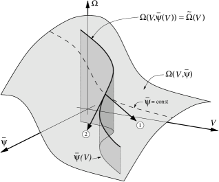
Figure 2: Relation between the two pressure definitions from Eqns. (21) and (IV.1) discussed in the text. In the first scheme the derivative is taken in the direction of increasing $V$ along a coordinate line of constant $\bar{\psi}$; in the second scheme the derivative is taken tangential to the submanifold $\Omega(V,\bar{\psi}(V))$, which emerges from restricting the values $(V,\bar{\psi})$ to the ones given by the defining equation $\bar{\psi}(V)$ of the linearization point.

After these considerations we can now proceed with our aim to derive a formula which gives the pressure in terms of the solution of the linear equation.

IV.2 The derivative of the functional

The same line of reasoning that led to Eqn. (II.3) can be employed to rewrite the derivative of the equilibrium grand potential as a derivative of the grand potential functional. If one again remembers that $\partial/\partial V$ just corresponds to a movement of the outer neutral cell boundary, the pressure definition (21) and Eqn. (14) give

$$\beta P_{\operatorname{lin}}^{(1)} = \sum_{i}\Big{[}-v_{i}\,n_{i}(R)\psi(R)+\frac{\bar{n}_{i}}{2}$$ (23)

$$\qquad+\;(1+v_{i}\bar{\psi})\,n_{i}(R)-\frac{1}{2}\frac{\big{(}n_{i}(R)\big{)}^{2}}{\bar{n}_{i}}\Big{]}_{\operatorname{eq}}$$

$$= \sum_{i}n_{i,{\operatorname{b}}}\,{\operatorname{e}}^{-v_{i}\bar{\psi}}\,\Big{[}1-v_{i}\big{(}\psi(R)-\bar{\psi}\big{)}$$

$$\qquad+\;\frac{1}{2}v_{i}^{2}\big{(}\psi(R)-\bar{\psi}\big{)}^{2}\Big{]}.$$

$$= \frac{1}{2}\sum_{i}n_{i}(R)\Big{[}\frac{n_{i}(R)}{\bar{n}_{i}}+\frac{\bar{n}_{i}}{n_{i}(R)}\Big{]}.$$ (24)

Eqn. (23) replaces Eqn. (8) and is easily recognized as its quadratic expansion about $\bar{\psi}$. Similarly, Eqn. (24) replaces Eqn. (9). Since $x+1/x\geq 2$, the expression (24) is larger than $\sum_{i}n_{i}(R)$, $i.\,e.$, the expression that would follow if the boundary density rule (9) would also hold in the linear case.

In the case of pressure definition (IV.1) we need the explicit volume dependence of $\Omega_{{\operatorname{lin}},{\operatorname{eq}}}$, which can again be rewritten as the derivative of functional $\Omega_{\operatorname{lin}}$, Eqn. (13). From Eqn. (12) follows immediately $\partial\bar{n}_{i}/\partial\bar{\psi}=-v_{i}\bar{n}_{i}$, and one readily obtains using Eqns. (13) and (14)

$$\frac{\partial\Omega_{{\operatorname{lin}},{\operatorname{eq}}}}{\partial\bar{\psi}}\;=\;\frac{\partial\Omega_{\operatorname{lin}}}{\partial\bar{\psi}}\bigg{|}_{\operatorname{eq}}\;=\;\frac{1}{2}V\Big{\langle}\big{(}\psi({\boldsymbol{r}})-\bar{\psi}\big{)}^{2}\Big{\rangle}\sum_{i}v_{i}^{3}\,\bar{n}_{i}.$$ (25)

Combining this with Eqn. (IV.1) results in an explicit formula for $P_{\operatorname{lin}}^{(2)}$:

$$\beta P_{\operatorname{lin}}^{(2)}\;=\;\beta P_{\operatorname{lin}}^{(1)}\,-\,\frac{1}{2}V\frac{{\operatorname{d}}\bar{\psi}}{{\operatorname{d}}V}\Big{\langle}\big{(}\psi({\boldsymbol{r}})-\bar{\psi}\big{)}^{2}\Big{\rangle}\sum_{i}v_{i}^{3}\,\bar{n}_{i}.$$ (26)

Note that unlike $P_{\operatorname{lin}}^{(1)}$ this expression depends on the whole potential distribution, and not just on the boundary potential or the boundary densities.

Equations (23,24) and (26) are a first key result of this paper. They replace the boundary density rule (9) from nonlinear PB theory, whose validity in the linear case has often falsely been taken for granted. In the second part of this article we will use these equations to derive explicit formulas—once we have established an optimal linearization point $\bar{\psi}$, which will be the topic of the next section.

V Optimal choice of $\bar{\psi}$

Up to now we have not specified the linearization point $\bar{\psi}$; rather, we have emphasized that its choice is largely at ones disposition. However, not all choices may be equally successful. In fact, the range of validity of linearization depends strongly on the choice of $\bar{\psi}$, since it is the difference between the potential and its linearization point that is required to be small and not the potential itself. This is particularly important in concentrated suspensions where this difference can be small even when the total potential is quite large.

In this section we identify an optimal linearization scheme—which however first requires a clarification of what “optimal” is supposed to mean. It proves instructive to first study the obvious (but futile) attempt to base optimality on a minimization of the grand potential, as we discuss in Sec. V.1. This sheds some surprising light onto traditional linearization. In Sec. V.2 we will then discuss a scheme based on the selfconsistently determined average potential and present its optimal aspects in Sec. V.3, which even though this approach has been used in the past RuBe81 ; TrHa96 ; TrHa97 ; GrRo01 have largely gone unnoticed.

V.1 Minimizing the grand potential?

One may try to obtain an optimal expansion point by looking for the value of $\bar{\psi}$ which minimizes the grand potential of linear theory. Let us thus set the derivative of $\Omega_{{\operatorname{lin}},{\operatorname{eq}}}$, Eqn. (20), with respect to $\bar{\psi}$ to zero. Using Eqn. (25) and remembering that $\langle(\psi({\boldsymbol{r}})-\bar{\psi})^{2}\rangle$ is nonzero unless the profile is completely flat, we see that the value of $\bar{\psi}$ at the extremum is given by the solution of $\sum_{i}v_{i}^{3}n_{i,{\operatorname{b}}}\,{\operatorname{e}}^{-v_{i}\bar{\psi}}=0$. The left hand side is a sum of strictly monotonically decreasing functions. If ions of both sign are present, the left hand side hence falls monotonically from $+\infty$ to $-\infty$ and the equation has a unique solution. Unfortunately, however, this monotonic decrease of the derivative also implies that this solution corresponds to a maximum of the grand potential. For a symmetric $v:v$ electrolyte the solution is for instance given by $\bar{\psi}=0$. The most widely used choice of the expansion point hence gives the largest grand potential of all possible linearization schemes (this can for instance be verified in Fig. 1 of Ref. GrRo01 , which shows the thermodynamic potential for various linearization schemes).

We hasten to remark that the above finding has to be put in the correct perspective. Minimization is only a meaningful venture if one can be sure about the existence of a lower bound . For instance, the PB functional is bounded below by the exact thermodynamic potential of the restricted primitive model. Minimizing the functional stems from the desire to get as close to this result as is possible within a mean field description DeHo01 . For the parameter $\bar{\psi}$ from linearized PB theory such a lower bound for the functional cannot be constructed, hence minimization is meaningless. And even if there were a bound, there would be no reason to approach it—unless one knows that it is favorably related to the actual thermodynamic potential.

V.2 Expansion about the average potential

Having seen that a minimization condition on $\Omega_{{\operatorname{lin}},{\operatorname{eq}}}$ is not successful, we will approach the problem from a different direction. If we average Eqn. (14) over the cell volume and use Eqn. (12), we find

$$\big{\langle}n_{i}({\boldsymbol{r}})\big{\rangle}\;=\;\bar{n}_{i}\,-\,v_{i}\,\bar{n}_{i}\big{\langle}\psi({\boldsymbol{r}})-\bar{\psi}\big{\rangle}.$$ (27)

If we were to choose $\langle\psi({\boldsymbol{r}})-\bar{\psi}\rangle=0$, the second term would vanish and the expansion points for the densities, $\bar{n}_{i}$, would coincide with the averages $\langle n_{i}({\boldsymbol{r}})\rangle$. It clearly makes sense to expand about these average values, since then the differences between actual value and expansion point can be kept small throughout the cell, $i.\,e.$, in the whole region in which linearization must work. Hence, the choice

$$\bar{\psi}\;=\;\bar{\psi}_{\operatorname{opt}}\;:=\;\langle\psi({\boldsymbol{r}})\rangle$$ (28)

is a particularly suitable one, which in anticipation of the results from Sec. V.3 we have labelled with the index “opt”.

At first sight this particular choice may seem difficult to work with, since the average $\langle\psi({\boldsymbol{r}})\rangle$ determines the value of $\bar{\psi}_{\operatorname{opt}}$, but the potential $\psi({\boldsymbol{r}})$ to be averaged is in turn the solution of the equation linearized about $\bar{\psi}_{\operatorname{opt}}$. However, the necessary selfconsistency is readily fulfilled, since $\langle\psi({\boldsymbol{r}})\rangle$ (and thus $\bar{\psi}_{\operatorname{opt}}$) does only depend on the state point and not on the actual ionic profile: For reasons of electroneutrality the total charge of all ions in the cell must be the negative of the colloid charge, and so we have

$$-\frac{Q}{V}\;=\;\sum_{i}v_{i}\langle n_{i}({\boldsymbol{r}})\rangle\;\stackrel{{\scriptstyle(\ref{eq:naverage},\ref{eq:psibopt})}}{{=}}\;\sum_{i}v_{i}\,n_{i,{\operatorname{b}}}\,{\operatorname{e}}^{-v_{i}\bar{\psi}_{\operatorname{opt}}}.$$ (29)

Satisfying this equation is necessary and sufficient for the validity of Eqn. (28), so we can determine $\bar{\psi}_{\operatorname{opt}}$ also from Eqn. (29). If the electrolyte contains ions of both sign, the right hand side monotonically decreases from $+\infty$ to $-\infty$ as a function of $\bar{\psi}_{\operatorname{opt}}$, so a solution always exists and is unique. For the special case of a $v:v$ electrolyte this equation reads

$$\frac{Q/vV}{2n_{\operatorname{b}}}\;\;\stackrel{{\scriptstyle v:v}}{{=}}\;\;\sinh(v\bar{\psi}_{\operatorname{opt}}).$$ (30)

V.3 Optimality of $\bar{\psi}_{\operatorname{opt}}$

The linearization scheme from the above Sec. V.2 has been put forward several times in the past RuBe81 ; TrHa96 ; TrHa97 ; GrRo01 , but various of its special properties have gone unnoticed. In this section we show, in which sense this scheme can be regarded as optimal.

Since the choice of $\bar{\psi}_{\operatorname{opt}}$ implies that the expansion points $\bar{n}_{i}$ coincide with the average microion densities $\langle n_{i}({\boldsymbol{r}})\rangle$, this translates to the corresponding screening constant $\bar{\kappa}_{\operatorname{opt}}$ which – as Eqn. (16) shows – is now also calculated with the average ionic strength within the cell:

$$\bar{\kappa}_{\operatorname{opt}}^{2}\;=\;4\pi\ell_{\operatorname{B}}\sum_{i}v_{i}^{2}\,\langle n_{i}({\boldsymbol{r}})\rangle.$$ (31)

Due to the Donnan effect the latter is different from the one in the reservoir, and it is more appropriate to have a linearization scheme which derives its screening constant from the actual ion densities in the macroion compartment. In fact, describing the colloidal system in an integral-equation approach together with the MSA closure yields an effective pair potential between colloids that is a screened Coulomb potential with the screening constant being equal to $\bar{\kappa}_{\operatorname{opt}}$—see for instance Ref. Bel00 .

Let us make the above remarks more explicit by specializing to a symmetric $v:v$ salt of concentration $n_{\operatorname{b}}$. The average counterion concentration is denoted by $\bar{n}_{\operatorname{c}}:=|Q|/vV$. In this case the optimal screening constant can be expressed as

$$\bar{\kappa}_{\operatorname{opt}}^{2} \stackrel{{\scriptstyle\text{(\ref{eq:kappab_v:v})}}}{{=}} \kappa^{2}\cosh(v\bar{\psi}_{\operatorname{opt}})$$ (32)

$$\stackrel{{\scriptstyle\text{(\ref{eq:psibopt_determine_v:v})}}}{{=}} 8\pi\ell_{\operatorname{B}}v^{2}n_{\operatorname{b}}\sqrt{1+(\bar{n}_{\operatorname{c}}/2n_{\operatorname{b}})^{2}}$$

$$= 4\pi\ell_{\operatorname{B}}v^{2}\sqrt{\bar{n}_{\operatorname{c}}^{2}+(2n_{\operatorname{b}})^{2}}.$$

This expression differs from the screening constant of the salt reservoir by also incorporating the contribution due to the counterions. It is illuminating to study its limiting behaviors at high and low salt. In the salt dominated regime, $i.\,e.$ $\bar{n}_{\operatorname{c}}\ll 2n_{\operatorname{b}}$, the screening constant $\bar{\kappa}_{\operatorname{opt}}$ is practically identical to the reservoir screening constant $\kappa$. This is the limit in which the Donnan effect is strongly diminished, and Eqn. (30) also shows that in this case $\bar{\psi}_{\operatorname{opt}}\rightarrow 0$. In the opposite limit of counterion domination, $\bar{n}_{\operatorname{c}}\gg 2n_{\operatorname{b}}$, the screening constant $\bar{\kappa}_{\operatorname{opt}}$ is essentially determined by the average counterion concentration, and it will be substantially larger than the screening constant of the reservoir. In this limit the Donnan effect is strong and $\bar{\psi}_{\operatorname{opt}}$ is significantly different from the zero. The traditional linearization scheme $\bar{\psi}=0$ will fail to adequately describe this case, even though the ionic profiles can be very flat and thus amenable to linearization. In summary, we see that linearizing the PB equation about $\bar{\psi}=0$ invariably ignores the counterion contribution to the screening, whereas the expansion about the selfconsistently determined average potential includes the counterions in a way that yields the correct behavior in the limits of high and low salt.

The fact that a strong Donnan effect goes along with a value of $\bar{\psi}_{\operatorname{opt}}$ substantially different from the reservoir potential is also to be expected on more fundamental grounds: The difference in microion concentrations across the membrane characteristic of the Donnan equilibrium implies a concomitant jump of the electrostatic potential, referred to as the “Donnan-potential”. Its magnitude can likewise be used to measure the strength of the Donnan effect. But a large Donnan-potential also results in a large average potential. This close connection between the Donnan-equilibrium and the optimal linearization scheme lead the authors of Ref. GrRo01 to suggest the name “Donnan-linearization” for the scheme from Eqn. (28).

The above findings can be succinctly reformulated in the following way: By choosing the optimal linearization point $\bar{\psi}_{\operatorname{opt}}$ the Donnan-equilibrium is automatically described correctly to lowest order. The solution of the linearized PB equation then provides the higher order corrections. We now show that every other linearization point gives a description that violates an important zeroth-order inequality valid on the nonlinear PB level. Let us first specialize to a $v:v$ electrolyte. If we denote by $\bar{n}_{\operatorname{c}}$ the average density of counterions and by $\bar{n}_{\operatorname{s}}$ the average density of salt molecules within the cell, we have within Poisson-Boltzmann theory

$$(\bar{n}_{\operatorname{c}}+\bar{n}_{\operatorname{s}})\,\bar{n}_{\operatorname{s}} = \langle n_{+}({\boldsymbol{r}})\rangle\,\langle n_{-}({\boldsymbol{r}})\rangle\;\stackrel{{\scriptstyle\text{(\ref{eq:Boltzmann})}}}{{=}}\;n_{\operatorname{b}}^{2}\,\langle{\operatorname{e}}^{-v\psi({\boldsymbol{r}})}\rangle\,\langle{\operatorname{e}}^{v\psi({\boldsymbol{r}})}\rangle$$ (33)

$$\geq n_{\operatorname{b}}^{2}\;{\operatorname{e}}^{-v\langle\psi({\boldsymbol{r}})\rangle}\;{\operatorname{e}}^{v\langle\psi({\boldsymbol{r}})\rangle}\;=\;n_{\operatorname{b}}^{2},$$

where Jensen’s inequality has been used. Eqn. (33) states that the mean ionic molarity Win95 within the suspension is greater than in the reservoir. On the other hand, within linearized Poisson-Boltzmann theory we find

$$(\bar{n}_{\operatorname{c}}+\bar{n}_{\operatorname{s}})\,\bar{n}_{\operatorname{s}} \stackrel{{\scriptstyle\text{(\ref{eq:lin_Boltzmann})}}}{{=}} n_{\operatorname{b}}^{2}\,\big{[}1-v\langle\psi({\boldsymbol{r}})-\bar{\psi}\rangle\big{]}\,\big{[}1+v\langle\psi({\boldsymbol{r}})-\bar{\psi}\rangle\big{]}$$ (34)

$$= n_{\operatorname{b}}^{2}\,\big{[}1-v^{2}\underbrace{\langle\psi({\boldsymbol{r}})-\bar{\psi}\rangle^{2}}_{\geq 0}\big{]}\;\;\leq\;\;n_{\operatorname{b}}^{2}.$$

This is the inequality (33) but with reversed inequality sign! Observe that linearizing about $\bar{\psi}_{\operatorname{opt}}$ is the only scheme that does not violate (33), since Eqn. (28) renders (34) an equality. The importance of these two inequalities can be further unveiled by solving them for the average salt concentration $\bar{n}_{\operatorname{s}}$ inside the suspension, which gives the sequence

$$\bar{n}_{\operatorname{s}}\big{|}_{\text{PB}}\;\geq\;\bar{n}_{\operatorname{s}}\big{|}_{\text{LPB, }\bar{\psi}_{\operatorname{opt}}}\;\geq\;\bar{n}_{\operatorname{s}}\big{|}_{\text{LPB}}$$ (35)

with

$$2\,\bar{n}_{\operatorname{s}}\big{|}_{\text{LPB, }\bar{\psi}_{\operatorname{opt}}}\;=\;\sqrt{\bar{n}_{\operatorname{c}}^{2}+(2\,n_{\operatorname{b}})^{2}}-\bar{n}_{\operatorname{c}}.$$ (36)

In other words: Linearized PB theory gives a lower bound to the average salt density within the cell, and $\bar{\psi}_{\operatorname{opt}}$ gives the largest lower bound. Since underestimating $\bar{n}_{\operatorname{s}}$ means overestimating the Donnan effect, the $\bar{\psi}_{\operatorname{opt}}$-scheme gives as close a representation of the Donnan equilibrium as is possible in a linear theory. Observe also that the prediction (36) for $\bar{n}_{\operatorname{s}}$ from Donnan linearization is indeed the well known formula describing the Donnan effect after neglecting activity coefficients (see for instance Ref. Ove56 ; Kek01 ). In that sense the set of inequalities (35) lies at the heart of the Donnan equilibrium and distinguishes $\bar{\psi}_{\operatorname{opt}}$ as optimal.

It is possible – although not straightforward – to extend the above considerations to general electrolyte compositions. In that case one has to look at more refined combinations of densities, also taking into account to what percentage a particular species is represented in the ionic mixture. One possibility is the following: Define the average

$${\mathscr{A}}\;:=\;\sum_{i}p_{i}\log\frac{\langle n_{i}({\boldsymbol{r}})\rangle}{n_{i,{\operatorname{b}}}}\quad\text{with}\quad p_{i}\;:=\;\frac{n_{i,{\operatorname{b}}}}{\sum_{j}n_{j,{\operatorname{b}}}},$$ (37)

which is inspired by a similar procedure employed when defining mean activity coefficients Win95 . Within PB theory we can readily derive

$${\mathscr{A}} \stackrel{{\scriptstyle\text{PB}}}{{=}} \sum_{i}p_{i}\log\big{\langle}{\operatorname{e}}^{-v_{i}\psi({\boldsymbol{r}})}\big{\rangle}$$ (38)

$$\geq -\sum_{i}p_{i}\,v_{i}\,\langle\psi({\boldsymbol{r}})\rangle\;\;=\;\;0,$$

where Jensen’s inequality has again been used. The last step follows from the charge neutrality of the salt reservoir. However, within linearized PB theory we get

$${\mathscr{A}} \stackrel{{\scriptstyle\text{LPB}}}{{=}} \sum_{i}p_{i}\log\big{\langle}{\operatorname{e}}^{-v_{i}\bar{\psi}}\big{[}1-v_{i}\big{(}\psi({\boldsymbol{r}})-\bar{\psi}\big{)}\big{]}\big{\rangle}$$ (39)

$$= \sum_{i}p_{i}\log\big{(}1-v_{i}\big{\langle}\psi({\boldsymbol{r}})-\bar{\psi}\big{\rangle}\big{)}$$

$$\leq -\sum_{i}p_{i}\,v_{i}\,\big{\langle}\psi({\boldsymbol{r}})-\bar{\psi}\big{\rangle}\;\;=\;\;0.$$

Here, the elementary inequality $\log(1+x)\leq x$ has been used. It is straightforward to see that the relations (38) and (39) reduce to (33) and (34) for a $v:v$ electrolyte. Nonlinear and linearized PB theory again lead to conflicting inequalities in all but one case: If $\bar{\psi}_{\operatorname{opt}}$ is chosen as the linearization point, the PB inequality is not infringed.

VI Explicit expressions and approximations for $d$-dimensional cell models

In Sec. IV we gave expressions of the pressure in terms of the charge- or potential-profiles that were based on the derivative of the grand potential. In this section we will substantiate these results by inserting the actual solution of the linearized PB equation for a $d$-dimensional cell model . We will place particular emphasis on the formulas that emerge from using the optimal linearization point $\bar{\psi}_{\operatorname{opt}}$ that we have discussed in the last section.

VI.1 Analytical formulas for the pressure

In the Appendix we outline how the linearized PB equation can be solved for a general $d$-dimensional cell model (where $d=1$, $2$, and $3$ corresponds to planar, cylindrical and spherical macroions, respectively). If we insert the final expression (54) into the pressure equation (23), we get the explicit formula

$$\beta P_{\operatorname{lin}}^{(1)}\;=\;\sum_{i}\bar{n}_{i}\,-\,\frac{1}{2}\Big{[}1-\gamma^{2}\Big{(}\frac{Q/V}{\sum_{i}v_{i}\,\bar{n}_{i}}\Big{)}^{2}\Big{]}\frac{\big{(}\sum_{i}v_{i}\,\bar{n}_{i}\big{)}^{2}}{\sum_{i}v_{i}^{2}\,\bar{n}_{i}},$$ (40)

where the variable $\gamma$ is defined as

$$\gamma\;:=\;\frac{1-\phi}{dD\sqrt{\phi}}$$ (41)

and $D$ is given in Eqn. (53). In the case of Donnan-linearization $-Q/V=\sum_{i}v_{i}\bar{n}_{i}$ according to Eqn. (29), such that Eqn. (40) further reduces to

$$\beta P_{\operatorname{lin}}^{(1)}\;\;\stackrel{{\scriptstyle\bar{\psi}_{\operatorname{opt}}}}{{=}}\;\;\sum_{i}\bar{n}_{i}\,-\,\frac{1}{2}\big{(}1-\gamma^{2}\big{)}\frac{\big{(}\sum_{i}v_{i}\,\bar{n}_{i}\big{)}^{2}}{\sum_{i}v_{i}^{2}\,\bar{n}_{i}}.$$ (42)

The case of the alternative pressure definition (IV.1) is less straightforward, since this depends explicitly on the whole potential distribution $\psi({\boldsymbol{r}})$ and not just just on its boundary value. According to Eqn. (26) the hard part is the integral over $(\psi({\boldsymbol{r}})-\bar{\psi}_{\operatorname{opt}})^{2}$, which is very unwieldy, as it contains products of modified Bessel functions. However, one can always numerically integrate this expression or – alternatively – numerically differentiate the grand potential $\Omega_{{\operatorname{lin}},{\operatorname{eq}}}$ from Eqn. (20).

The explicit pressure formulas (40) and (42) are a further key result of this paper, and in the remainder we will study some of their consequences. Unfortunately, due to the algebraic complexity their properties cannot be readily seen. In the next subsection we will therefore spend some time to study their analytical behavior in a few important limiting cases. Finally we will provide graphical illustrations for the pressure formulas (40) and (42) as well as the pressure definition (IV.1) for several exemplary cases in Sec. VII.

VI.2 Pressure bounds, limiting behavior and expansions

The pressure formula (23) is quadratic in $\psi(R)$, and it is easily checked that it takes its minimum value at the inhomogeneity $\psi_{\operatorname{i}}$ defined in Eqn. (17). From Eqn. (54) and the definition of $\gamma$ in Eqn. (41) we see that this formally corresponds to $\gamma=0$, and indeed the pressure expression (40) attains its minimum value there. For a symmetric $v:v$ electrolyte this implies for the excess osmotic pressure

$$\frac{\beta\,\Delta P_{{\operatorname{lin}},\text{min}}^{(1)}}{2n_{\operatorname{b}}} := \frac{\beta(P_{{\operatorname{lin}},\text{min}}^{(1)}-P_{\text{res}})}{2n_{\operatorname{b}}}$$ (43)

$$= \cosh(v\bar{\psi})-\frac{1}{2}\sinh(v\bar{\psi})\tanh(v\bar{\psi})-1$$

$$= \frac{\big{[}\cosh(v\bar{\psi})-1\big{]}^{2}}{2\cosh(v\bar{\psi})}\;\geq\;0.$$

Hence, in the symmetric case the pressure from linearized PB theory defined via Eqn. (21) is nonnegative for every chosen linearization point $\bar{\psi}$. However, this does not hold for general electrolytes. It may be verified that for the asymmetric case of a $1:2$ electrolyte the excess pressure is negative if $\bar{\psi}$ has the same sign as the divalent ion species and $|\bar{\psi}|\in[0;0.6309]$. In Donnan-linearization this comes down to the requirement that $Q$ has the same sign as the divalent species and $0\leq|Q|\leq 1.596n_{\operatorname{b}}V$, where $n_{\operatorname{b}}$ is the reservoir density of the monovalent species. Essentially, the pressure can become negative when the counterion content within the cell is overwhelmed by the salt ions.

Let us now restrict again to a symmetric $v:v$ electrolyte and define the parameter

$$\theta\;:=\;\frac{|Q|/vV}{2n_{\operatorname{b}}}\;=\;\frac{\bar{n}_{\operatorname{c}}}{2n_{\operatorname{b}}}.$$ (44)

This ratio between average counterion concentration and salt reservoir concentration measures whether we are in the salt dominated regime ($\theta$ small) or the counterion dominated regime ($\theta$ large). Using $\theta$, Eqn. (32) can be rewritten as $\bar{\kappa}_{\operatorname{opt}}^{2}=\kappa^{2}\sqrt{1+\theta^{2}}$. The definition (44) shows that $\theta$ is small if either $V$ is large ($i.\,e.$, the volume fraction of colloids is low) or $n_{\operatorname{b}}$ is large ($i.\,e.$, much salt has been added to the system). In both cases $\bar{\kappa}_{\operatorname{opt}}R$ becomes large and we may exploit the asymptotic behavior of the modified Bessel functions AbSt70 to approximate the quantity $D$ from Eqn. (53) according to

$$D \simeq {\operatorname{K}}_{d/2}(\bar{\kappa}_{\operatorname{opt}}r_{0})\,{\operatorname{I}}_{d/2}(\bar{\kappa}_{\operatorname{opt}}R)$$

$$\simeq \frac{{\operatorname{K}}_{d/2}(\bar{\kappa}_{\operatorname{opt}}r_{0})}{\sqrt{2\pi\bar{\kappa}_{\operatorname{opt}}R}}\,{\operatorname{e}}^{\bar{\kappa}_{\operatorname{opt}}R}.$$

$$\stackrel{{\scriptstyle\bar{\kappa}_{\operatorname{opt}}r_{0}\gg 1}}{{\simeq}} \frac{{\operatorname{e}}^{\bar{\kappa}_{\operatorname{opt}}(R-r_{0})}}{2\bar{\kappa}_{\operatorname{opt}}\sqrt{Rr_{0}}}$$

Hence, $\gamma\propto 1/D$ vanishes exponentially. The pressure $P_{\operatorname{lin}}^{(1)}$ will thus approach its minimum value computed above. Since in this limit $\bar{\psi}_{\operatorname{opt}}\rightarrow 0$, we may expand Eqn. (43) for small $\bar{\psi}_{\operatorname{opt}}$ and obtain

$$\frac{\beta\,\Delta P_{{\operatorname{lin}},\text{min}}^{(1)}}{2n_{\operatorname{b}}}\;\stackrel{{\scriptstyle\theta\ll 1}}{{\simeq}}\;\frac{(v\bar{\psi}_{\operatorname{opt}})^{4}}{8}\;\stackrel{{\scriptstyle(\ref{eq:psibopt_determine_v:v})}}{{\simeq}}\;\frac{\theta^{4}}{8},$$ (45)

showing that the excess osmotic pressure (measured in units of the reservoir concentration) vanishes as the fourth power of $\theta$. We note in passing that the lowest order calculation based merely on the average counterion concentration $\bar{n}_{\operatorname{c}}$ from Eqn. (36) (or, alternatively, the boundary density from salt-free PB theory HaPo01 ) gives instead the asymptotic behavior $\theta^{2}/2$, $i.\,e.$, only a quadratic dependence.

The full expression (42) contains a term which appears to be of second order in $\theta$, namely $\theta^{2}\gamma^{2}/2$. Since $\gamma$ vanishes exponentially, one could be led to the incorrect conclusion (by “prematurely” terminating the expansion at this point) that the pressure in linearized PB theory also vanishes exponentially RuBe81 . While it is in fact true that in the full nonlinear theory the pressure vanishes exponentially in the limit of salt-domination (a simple plausibility argument for this can be found in Ref. DeHo01 ), this does not hold for the linearized theory , where the exponential decay of the term $\theta^{2}\gamma^{2}/2$ is masked by the quartic asymptotic from Eqn. (45). In any case, one has to be a little bit careful about the physical meaning of this limit. It indeed correctly describes a single charged colloid immersed in an electrolyte. However, a dilute suspension of many colloids is not well described in this limit, since the lack of mutual repulsions renders some basic assumptions about the cells questionable. Furthermore, one must keep in mind that our formulas only give the osmotic pressure of the suspension due to the microions. Even though this contribution most often dominates just because there are many more microions than macroions, the contribution of the latter has to become dominant once the microion term vanishes exponentially.

The limit of large volume fraction, $\phi\rightarrow 1$, requires a little more care. Using $R=r_{0}\phi^{-1/d}$, an expansion of $D$ around $\phi=1$ gives to lowest order

$$D \stackrel{{\scriptstyle\phi\rightarrow 1}}{{\simeq}} \frac{x_{0}}{2}\bigg{\{}{\operatorname{K}}_{\nu+1}(x_{0})\Big{[}{\operatorname{I}}_{\nu}(x_{0})+{\operatorname{I}}_{\nu+2}(x_{0})\Big{]}$$

$$+\;{\operatorname{I}}_{\nu+1}(x_{0})\Big{[}{\operatorname{K}}_{\nu}(x_{0})+{\operatorname{K}}_{\nu+2}(x_{0})\Big{]}\bigg{\}}\times(\phi^{-1/d}-1),$$

with $\nu=d/2-1$ and $x_{0}=\bar{\kappa}_{\operatorname{opt}}r_{0}=\kappa r_{0}(1+\theta^{2})^{1/4}$. Since $\theta\propto 1/(1-\phi)$, both $\theta$ and $x_{0}$ diverge as $\phi\rightarrow 1$. $x_{0}/2$ times the expression in curly brackets approaches $1-c/x_{0}^{2}$ with $c=(d^{2}-1)(d^{2}+3)/64$ AbSt70 . The term $\gamma$ therefore behaves asymptotically like

$$\gamma\;\stackrel{{\scriptstyle\phi\rightarrow 1}}{{\simeq}}\;\frac{1-\phi}{d(1-c/x_{0}^{2})(\phi^{-1/d}-1)\sqrt{\phi}}\;\simeq\;1+\frac{c}{x_{0}^{2}}.$$ (46)

This shows that $1-\gamma^{2}$ is of order $1/\theta$. Using this, it is now straightforward to show that to lowest order the high volume fraction limit of Eqn. (40) is given by

$$\beta P_{\operatorname{lin}}^{(1)}\;\stackrel{{\scriptstyle\phi\rightarrow 1}}{{\simeq}}\;\bar{n}_{\operatorname{c}}.$$ (47)

This equation is simple to interpret: It states that the pressure is given by the average counterion density. This is reasonable, because in this limit the ionic profiles become flat and thus the electrolyte ideal. Indeed, Eqn. (47) merely states that the osmotic coefficient goes to 1. We hasten to add that Eqn. (47) only demonstrates the proper behavior within the cell model. Real suspensions crystallize at large enough volume fraction, a transition which can only be described correctly once one accounts for the ordered phase as well—see for instance Refs. HoAl83 ; ShAk87 ; ReBe97 ; KuDi97 ; RoHa97 ; RoDi99 . But in order to get the phase boundary right, one of course also needs a good estimate of the grand potential in the fluid phase, so the correct scaling of the optimal linearization at high volume fraction is after all practically important.

Within Donnan-linearization positivity of the pressure does not generally hold for the second pressure definition (IV.1), not even for symmetric electrolytes. For a $v:v$ electrolyte this can be seen by differentiating Eqn. (30) with respect to $V$ and inserting into Eqn. (26), whereby one obtains

$$\frac{\beta(P_{\operatorname{lin}}^{(2)}-P_{\operatorname{lin}}^{(1)})}{2n_{\operatorname{b}}}\;=\;-v^{2}\,\frac{\sinh^{2}v\bar{\psi}_{\operatorname{opt}}}{2\cosh\bar{\psi}_{\operatorname{opt}}}\big{\langle}\big{(}\psi({\boldsymbol{r}})-\bar{\psi}_{\operatorname{opt}}\big{)}^{2}\big{\rangle},$$ (48)

which is clearly negative. In the limit of low volume fraction or high salt $\bar{\psi}_{\operatorname{opt}}$ tends to zero, and expression (48) scales like $(v\bar{\psi}_{\operatorname{opt}})^{2}=\theta^{2}$ times factors that do not tend to zero. It hence does not vanish as quickly as $P_{\operatorname{lin}}^{(1)}\sim\theta^{4}$ and the pressure $P_{\operatorname{lin}}^{(2)}$ must become negative in this limit. We finally note that for asymmetric electrolytes $P_{\operatorname{lin}}^{(2)}$ can also become negative, but will not always be smaller than $P_{\operatorname{lin}}^{(1)}$.

Let us close with a few remarks on the pressure in the traditional linearization scheme $\bar{\psi}=0$. Since the linearization point is volume-independent, the two pressure definitions (21) and (IV.1) coincide. If one calculates the excess osmotic pressure by inserting $\bar{\psi}=0$ into Eqn. (23), one finds that the zeroth order is canceled by the reservoir pressure, while the first order drops out due to reservoir electroneutrality, giving

$$\beta\,\Delta P_{\operatorname{lin}} \stackrel{{\scriptstyle\bar{\psi}=0}}{{=}} \frac{1}{2}\psi(R)^{2}\sum_{i}v_{i}^{2}n_{i,{\operatorname{b}}}$$ (49)

$$\stackrel{{\scriptstyle(\ref{eq:psi(R)})}}{{=}} \frac{(Q/V)^{2}}{2\sum_{i}v_{i}^{2}n_{i,{\operatorname{b}}}}\,\gamma^{2}.$$

In the special case of a $v:v$ electrolyte this simplifies further to $\beta\Delta P_{\operatorname{lin}}/2n_{\operatorname{b}}=\theta^{2}\gamma^{2}/2$ (recognize the “second order” term from above!). Eqn. (49) shows that this pressure is always positive. Moreover, in the limit of low $\phi$ or large salt it vanishes exponentially as $\gamma^{2}\sim\exp\{-2\kappa R\}$ – just as in full PB theory. Even though $\bar{\psi}_{\operatorname{opt}}$ also approaches zero in this limit, the corresponding pressure asymptotics is dominated by the way in which it does so, yielding a power law as discussed above. In the opposite limit of large $\phi$ we have seen above that $\gamma\rightarrow 1$, hence for the $v:v$ case the pressure using $\bar{\psi}=0$–linearization asymptotically behaves like $\beta\Delta P_{\operatorname{lin}}\sim\bar{n}_{\operatorname{c}}^{2}/4n_{\operatorname{b}}$, $i.\,e.$, it diverges quadratically in $\bar{n}_{\operatorname{c}}$ and not linearly as it should. We finally note that a quadratic expression like (49) has recently been rederived in Ref. ZhCz01 by using a perturbative expansion of the PB equation and restricting to lowest order. However, in this approach it is difficult to see that this is in fact thermodynamically consistent.

VII Exemplary comparison with nonlinear PB theory

In this section we provide a comparison of the above pressure formulas with the results from nonlinear PB theory , which is intended to clarify and illustrate the findings from the last sections. Apart from the pressure, we will also calculate the compressibility, which is defined as ${\mathscr{K}}=\frac{1}{V}(\partial V/\partial\Delta P)$. For a graphical representation it is however more convenient to plot the reduced inverse compressibility $\partial\beta\Delta P/\partial\bar{n}_{\operatorname{c}}=1/\bar{n}_{\operatorname{c}}k_{\operatorname{B}}T{\mathscr{K}}$, where the average density of counterions is again defined by $\bar{n}_{\operatorname{c}}=|Q|/vV$.

In order to underline the generality of the formulas derived above, we will use the following three different situations: ($i$) spherical colloids in a 1:1 electrolyte, ($ii$) cylindrical colloids in a 1:1 electrolyte, and ($iii$) spherical colloids in a 1:2 electrolyte.

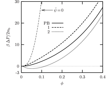
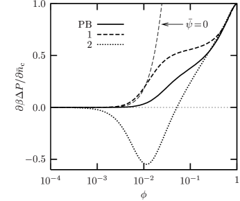
Figure 3: Pressure (left) and inverse reduced compressibility (right) as a function of volume fraction $\phi$ for a solution of spherical colloids having a bare charge $Q=3500\,e$ and a radius $r_{0}=133\,\text{nm}$. The system is in contact with a dilute 1:1 electrolyte of concentration $3.6\,\mu\text{M}$ and the Bjerrum length is $\ell_{\operatorname{B}}=\,0.714\,\text{nm}$, corresponding to water at room temperature. The solid curve is the result from nonlinear PB theory, the bold dashed curve is the first pressure definition (23) combined with the optimal linearization from Sec. V (leading to the explicit expression (42)) while the dotted curve combines this scheme with the second pressure definition (26). The fine dashed curve uses $\bar{\psi}=0$, in which case both pressure definitions coincide, leading to the explicit formula (49).

The first system we study consists of spherical colloids of charge $Q=3500\,e$ and radius $r_{0}=133\,\text{nm}$ immersed in an aqueous solution ($i.\,e.$, $\ell_{\operatorname{B}}=\,0.714\,\text{nm}$) which is dialyzed against a 1:1 electrolyte of rather low molarity $3.6\,\mu\text{M}$. Motivated by the prediction of a gas-liquid phase separation at these parameters RoDi99 , the authors of Ref. GrRo01 used them as an illustration which pushes linearized theory to the limits of validity, making the way in which it deviates from PB theory particularly visible. Lowering the colloidal charge entails a successively better agreement between linear and nonlinear theory, as can also be seen in Ref. GrRo01 .

Fig. 3 shows the pressure (left) and the inverse reduced compressibility (right) as a function of volume fraction $\phi$. The solid line corresponds to the solution of the nonlinear PB equation. The pressure is given by Eqn. (9) and the excess pressure is always positive (see Eqn.(11)). The same holds for the compressibility . The dashed and dotted curves correspond to the solutions from linearized PB theory. For $\bar{\psi}=0$ both pressure definitions (21) and (IV.1) coincide, but in this case the predictions are clearly off from the PB result except at very low volume fraction. In contrast, using the optimal linearization point $\bar{\psi}_{\operatorname{opt}}$ from Sec. V.2 brings about the correct behavior at high volume fraction, $i.\,e.$, in the regime where the cell model is particularly appropriate and linearization should indeed work because of relatively flat ionic profiles.

The pressure definition (IV.1) – the total derivative of the grand potential $\Omega(V,T,\ldots,\bar{\psi}_{\operatorname{opt}}(V))$ with respect to volume – corresponds to the one employed in Ref. GrRo01 . It can be seen to lead to negative pressures and compressibilities at moderately low volume fractions, which would imply a segregation into a dense and a dilute colloidal phase. Such a phase transition has also been claimed in other recent theoretical works RoHa97 ; RoDi99 ; War00 which likewise are essentially based on linearized PB theory. However, the similarity of the resulting phase diagrams, the appearance of essentially the same “volume terms” in the grand potential (which here are responsible for the effect), and the fact that full PB theory does not show any phase transition, lead the authors of Ref. GrRo01 to question these claims of a gas-liquid coexistence in such systems as a spurious side effect of linearization. In a similar spirit, Diehl $et\,al.$ DiBa01 show (within a generalized Debye-Hückel-Bjerrum approach LeBa98 ; TaLe98_2 ) that explicitly re-incorporating the effects of counterion condensation, which are neglected when doing the linearization, removes (or at least strongly suppresses) the phase transition otherwise clearly visible. We remark that Fig. 1 of Ref. DiBa01 , showing the excess osmotic pressure as a function of volume fraction for a salt-free suspension of spherical colloids with varying bare charge, can be reproduced almost quantitatively within the cell model by using Donnan-linearization and employing the pressure definition (IV.1). While these warnings about the dangers of linearization are certainly well made, we want to point out that things are in fact even a little more subtle: Not even linearized theory needs to show the phase transition. Whether or not it does so depends crucially on the pressure definition as well as the linearization point. For $\bar{\psi}=0$ there is no phase transition. For $\bar{\psi}=\bar{\psi}_{\operatorname{opt}}$ there is a phase transition only if pressure definition (IV.1) is used. The definition (21) – which is based on the partial derivative of the grand potential with respect to volume – yields a positive compressibility.

Let us repeat that this pressure definition (21) could only be written down once the linearization point has been recognized as an independent variable. And since it is the volume-dependence of $\bar{\psi}_{\operatorname{opt}}$ that renders $P_{\operatorname{lin}}^{(2)}$ negative, it must also be related to the “volume” terms discussed in Refs. RoHa97 ; RoDi99 ; War00 ; GrRo01 (see also Ref. Cha01 ). Our formulation of the problem hence illustrates that the way in which these terms drive a phase transition is closely related to the choice which variables one intends to keep constant when differentiating the thermodynamic potential. Within the cell model it is obvious that PB theory only yields positive pressures and which pressure definition is hence preferrable, but when relaxing the constraints of a cell model or mean field PB theory the nature of effective interactions is much less obvious. See for instance Ref. Bel00 for a recent critical evaluation of the theoretically as well as experimentally subtle issue of phase separation in suspensions of spherical colloids.

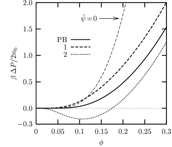
Figure 4: Same plots as in Fig. 3, but for cylindrical macroions having a charge parameter $\xi=4.2$ ($i.\,e.$, 4.2 charges along the axis per Bjerrum length) and a radius $r_{0}=1.2\,\text{nm}$ (those values correspond roughly to DNA). The system is in contact with a dilute 1:1 electrolyte of physiological salt concentration $100\,\text{mM}$. The line styles are the same as in Fig. 3.

In our next example we turn to a physical system which differs in the geometry of the colloids and which is (quite literally) of vital importance. Fig. 4 shows pressure and compressibility of an aqueous solution of cylindrical colloids, $i.\,e.$, charged rods, which have a radius of $r_{0}=1.2\,\text{nm}$ and a line charge density of 1 charge per $1.7\,\text{\AA}$ (or 4.2 charges per Bjerrum length) dialyzed against an 1:1 electrolyte of concentration $100\,\text{mM}$. The colloid is much stronger charged than in the spherical situation above, in the sense that the surface charge density is a factor 50 larger. On the other hand, the salt concentration is also much larger (with the reservoir screening length being only 0.6% of the screening length in the above low-salt case) which keeps the potentials low. The above choice of values corresponds to DNA in a physiological salt environment. As Fig. 4 shows, nonlinear PB theory again gives positive pressure and compressibility for all volume fractions $\phi$, and the large-$\phi$ behavior is captured correctly if Donnan linearization is employed, while the choice $\bar{\psi}=0$ fails there. However, using $\bar{\psi}_{\operatorname{opt}}$ and the definition (IV.1) results in a pressure that is negative for $\phi\lesssim 17\%$ and a negative compressibility for $\phi\lesssim 11\%$. If this were true, all DNA in animal cells would tend to aggregate and phase separate! But again, this failure is not an inevitable artifact of linearization, since the pressure $P_{\operatorname{lin}}^{(1)}$ is perfectly positive and gives rise to positive compressibilities. Incidentally, DNA can be condensed, but this requires multivalent ions Blo91 and is known to be a correlation effect which is missing in PB theory, see for instance GuNi86 ; LyNo97 ; GrMa97 .

Poisson-Boltzmann theory and the linearization scheme employing $\bar{\psi}=0$ predict an exponentially vanishing pressure as $\phi\rightarrow 0$. However, as we have remarked above the pressure due to the macroions has to become significant at some point (see Ref. RaCo00 for measurements on DNA in low salt solutions which appear to support this view). For linear polyelectrolytes this is even more relevant than for spherical colloids, since the conformational degrees of freedom and the degree of entanglement becomes important DoCo95 .

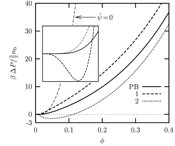
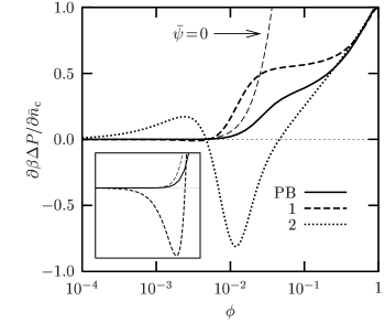
Figure 5: Same plots as in Fig. 3, but for a 1:2 electrolyte. The colloid charge has the same sign as the divalent ions, the reservoir density of the monovalent ions is $3.6\,\mu\text{M}$. The inset in the left panel magnifies the regions $[0;0.008]\times[-0.003;0.003]$, while the inset on the right magnifies $[10^{-4};10^{-2}]\times[-0.01;0.005]$, showing that in this example the first pressure definition (21) also gives negative pressures and compressibilities, while the PB result does not.

In our final example we study an asymmetric electrolyte. We go back to the system of spherical colloids studied above and replace the ions of one sign by divalent ones, $i.\,e.$, we assume a 1:2 electrolyte of concentration $3.6\,\mu\text{M}$, which in particular implies that the divalent species occurs with a concentration of $1.8\,\mu\text{M}$ in the reservoir. According to the discussion in Sec. VI.2 the case in which the colloid has the same sign of charge as the divalent ions is particularly interesting, since then positivity of the pressure cannot be guaranteed even for the pressure definition (21). For this case Fig. 5 shows again pressure and compressibility as a function of volume fraction. PB theory is once more found to give positive results, and the same remarks as above about the poor high-$\phi$ behavior of the linearization point $\bar{\psi}=0$ compared to $\bar{\psi}=\bar{\psi}_{\operatorname{opt}}$ apply also here.

However, there is an (expected) difference concerning the behavior of $P_{\operatorname{lin}}^{(1)}$, which becomes (very slightly) negative for $\phi\lesssim 0.68\%$ and gives rise to negative compressibility for $\phi\lesssim 0.51\%$, as is illustrated in the insets. In Sec. VI.2 we have seen that the pressure can become negative if $|Q|\leq 1.596n_{\operatorname{b}}V$, which in this case implies $\phi\lesssim 0.96\%$ – and indeed, lowering $\phi$ by further 30% brings about the negative pressure. We mention in passing that with a colloid having the opposite sign of charge as the divalent species this does not occur.

VIII Conclusion and summary

The main motivation of the present paper has been the following question: How can the membrane pressure due to a Donnan-equilibrium best be described within linearized PB theory? This first required a clarification of ($i$) how one computes the pressure and ($ii$) what one means by “best”. Often the pressure has been computed (without much justification) by using the predictions of the linearized PB equation in formulas of the nonlinear theory (or expansions thereof); moreover, this recourse to the full theory is not unique and hence prone to inconsistencies. These problems are avoided by starting from the appropriate thermodynamic potential functional of linear theory, which however still leaves two alternative definitions for the pressure that differ in their treatment of a possible volume dependence of the linearization point. Neither definition predicts the pressure to be proportional to the density of microions at the outer cell boundary, $i.\,e.$, the well known result from nonlinear PB theory does not apply on the linearized level. All this can be discussed without fixing the expansion point, but optimality considerations nevertheless suggest a specific choice for it. Explicit formulas can be obtained, since the linearized PB equation can be solved analytically for general cell models.

Let us thus sumarize the key findings of this work:

(a) Linearized PB theory can be based on a density functional which is the quadratic expansion of the well known functional of nonlinear PB theory. The choice of the expansion point distinguishes different linearization schemes. The equilibrium value of this functional is the thermodynamic potential, in our case the grand potential.

(b) The pressure is given by the volume derivative of this thermodynamic potential. There is a choice as to whether or not one would like to keep the linearization point fixed, resulting in two different pressure definitions both based on the thermodynamic potential.

(c) The boundary density rule (9) from nonlinear PB theory is replaced by the quadratic expansion of the nonlinear formula in the boundary potential.

(d) The range of validity of linearization depends on the expansion point. We proved that linearization about the selfconsistently determined average potential is optimal—in the sense that it automatically describes the Donnan effect correctly in lowest order, leaving the linearized PB equation to incorporate higher order corrections. Furthermore, we showed that all other linearization schemes violate an important inequality from nonlinear PB theory related directly to the Donnan effect.

(e) The linearized PB equation can be solved exactly for symmetric cell models of arbitrary dimension, salt reservoir composition and linearization point. We used this solution to derive explicit formulas for the pressure and have discussed their analytical properties in detail.

(f) A comparison with the results from nonlinear PB theory has been performed, showing that the validity of linearization depends strongly on the linearization point. While the traditional linearization scheme completely fails to describe the important limit of large volume fraction, the optimal (Donnan-) linearization becomes asymptotically correct there.

(g) For pressure definition (IV.1), $i.\,e.$ the total volume derivative of the grand potential, negative pressures and compressibilities can occur. These findings have previously been taken as indications of a gas-liquid phase separation in suspensions of spherical colloids. In the present work we showed that the same theoretical reasoning would predict DNA to phase separate under physiological conditions at all relevant concentrations. We consider this as a further striking argument against the genuineness of the transition.

(h) In nonlinear PB theory the pressure is always positive. Whether or not this still holds on the linearized level depends crucially on the precise definition of the pressure itself. It is for this reason that we advocate defining the pressure via the partial derivative of the grand potential with respect to the volume ($i.\,e.$, keeping in particular the linearization point fixed), since the pressure is then always positive for symmetric electrolytes—in agreement with nonlinear PB theory.

Appendix A Solution of the linear PB equation for a cell model in $d$ dimensions

Consider a cell model in $d$ dimensions with generalized radial coordinate $r$. $d=1$, $2$, and $3$ corresponds to planar, cylindrical and spherical macroions, respectively. After the transformation $x=\bar{\kappa}r$ and $\psi(r)=\tilde{\psi}(\bar{\kappa}r)=\tilde{\psi}(x)$ the linearized PB equation (15) reads

$$\tilde{\psi}^{\prime\prime}(x)+\frac{d-1}{x}\,\tilde{\psi}^{\prime}(x)\;=\;\tilde{\psi}(x)-\psi_{\operatorname{i}},$$ (50)

where the prime indicates differentiation with respect to $x$. Henceforth we will not bother with the difference between $\tilde{\psi}$ and $\psi$ and omit the tilde. An obvious particular solution of Eqn. (50) is $\psi(x)=\psi_{\operatorname{i}}$, while the homogeneous equation is solved by the ansatz $\psi(x)=w(x)/x^{\nu}$ with $\nu=d/2-1$, provided $w(x)$ solves the Bessel equation $x^{2}\,w^{\prime\prime}(x)+x\,w^{\prime}(x)-(x^{2}+\nu^{2})\,w(x)=0$. Two linearly independent solutions are the modified Bessel functions ${\operatorname{K}}_{\nu}$ and ${\operatorname{I}}_{\nu}$ AbSt70 . The general solution of the differential equation (50) can therefore be written as

$$\psi(x)=\psi_{\operatorname{i}}+C_{\operatorname{K}}\,\frac{{\operatorname{K}}_{\nu}(x)}{x^{\nu}}+C_{\operatorname{I}}\,\frac{{\operatorname{I}}_{\nu}(x)}{x^{\nu}},$$ (51)

where $C_{\operatorname{K}}$ and $C_{\operatorname{I}}$ are constants to be determined by the following boundary conditions. Gauss’ law relates the radial derivative of the electrostatic potential at $r_{0}=x_{0}/\bar{\kappa}$ to the surface charge density $e\sigma$ of the macroion. If we define the latter to be the total charge of the macroion divided by its surface area, we have $\psi^{\prime}(x_{0})=-4\pi\ell_{\operatorname{B}}\sigma/\bar{\kappa}$. Since the whole cell is neutral, we also have $\psi^{\prime}(X)=0$ at the outer cell radius $R=X/\bar{\kappa}$. The integration constants now follow from inserting these boundary conditions into the general solution. After a little algebra we then find the potential

$$\psi(x) = \psi_{\operatorname{i}}+\frac{4\pi\ell_{\operatorname{B}}\sigma}{\bar{\kappa}D}\left(\frac{x_{0}}{x}\right)^{\nu}$$ (52)

$$\times\,\Big{[}{\operatorname{I}}_{\nu+1}(X){\operatorname{K}}_{\nu}(x)+{\operatorname{K}}_{\nu+1}(X){\operatorname{I}}_{\nu}(x)\Big{]},$$

where the determinant $D$ is defined as

$$D\;=\;{\operatorname{K}}_{\nu+1}(x_{0}){\operatorname{I}}_{\nu+1}(X)-{\operatorname{K}}_{\nu+1}(X){\operatorname{I}}_{\nu+1}(x_{0}).$$ (53)

We have $D>0$ since $X>x_{0}$.

At the outer boundary the potential (52) can be further simplified. The term in angular brackets reduces to $1/X$, and using the volume fraction $\phi$ the surface charge density can be rewritten in terms of the colloid charge as $\sigma/r_{0}=(Q/V)(1-\phi)/d\phi$. Inserting the definitions (16) for $\bar{\kappa}$ we arrive at

$$\psi(R)\;=\;\psi_{\operatorname{i}}+\frac{Q/V}{\sum_{i}v_{i}^{2}\,\bar{n}_{i}}\frac{1-\phi}{dD\sqrt{\phi}}.$$ (54)

Equation (54) gives the boundary potential in linearized PB theory for a general $d$-dimensional cell model with arbitrary linearization point $\bar{\psi}$ and electrolyte composition.

References

- (1) R. J. Hunter, Introduction to Modern Colloid Science, Oxford University Press, Oxford (1994).
- (2) H. Dautzenberg, W. Jaeger, J. Kötz, B. Philipp, Ch. Seidel and D. Stscherbina, Polyelectrolytes. Formation, Characterization and Application, Carl Hanser, München (1994).
- (3) H. Lodish, A. Berk, S. L. Zipursky, P. Matsudaira, D. Baltimore, and J. Darnell, Molecular Cell Biology, 4th ed., W. H. Freeman, New York (2001).
- (4) F. Oosawa, Polyelectrolytes, Marcel Dekker, New York (1971);
- (5) W. B. Russel, D. A. Saville, and W. R. Schowalter, Colloidal Dispersions, Cambridge University Press, New York (1989).
- (6) D. F. Evans and H. Wennerström, The Colloidal Domain, 2nd ed., Wiley, New York (1999);
- (7) T. Radeva (ed.), Physical Chemistry of Polyelectrolytes, Surfactant Science Series, vol. 99, Marcel Dekker, New York (2001).
- (8) A. Katchalsky, Pure Appl. Chem. 26, 327, (1971).
- (9) J.-L. Barrat and J.-F. Joanny, Theory of Polyelectrolyte Solutions, in: Advances in Chemical Physics, vol. 94, ed. by I. Prigogine and S. A. Rice, Wiley (1996).
- (10) J.-P. Hansen and H. Löwen, Annu. Rev. Phys. Chem. 51, 209 (2000).
- (11) L. Belloni, J. Phys.: Condens. Matter 12, R549 (2000).
- (12) D. Andelman in: Handbook of Biological Physics, I, ed. by R. Lipowsky and E. Sackmann, Elsevier (1995), Chapter 12.
- (13) V. A. Parsegian and D. Gingell, Biophys. J. 12, 1192 (1972);
- (14) W. B. Russel and D. W. Benzing, J. Colloid Interface Sci. 83, 163 (1981).
- (15) M. Strauss, T. A. Ring, and H. K. Bowen, J. Colloid Interf. Sci. 118, 326 (1987).
- (16) P. L. Hansen, R. Podgornik, and V. A. Parsegian, Phys. Rev. E 64 021907 (2001).
- (17) S. Levine, J. Chem. Phys. 7, 831 (1939).
- (18) S. L. Brenner and R. E. Roberts, J. Phys. Chem. 77, 2367 (1973).
- (19) E. S. Reiner and C. J. Radke, J. Chem. Soc. Farad. Trans. 86, 3901 (1990).
- (20) H. Löwen, J.-P. Hansen, and P. A. Madden, J. Chem. Phys. 98 3275 (1993).
- (21) R. A. Marcus, J. Chem. Phys. 23, 1057 (1955).
- (22) E. Trizac and J.-P. Hansen, J. Phys. Cond. Mat. 8, 9191 (1996).
- (23) E. Trizac and J.-P. Hansen, Phys. Rev. E 56, 3137 (1997).
- (24) H. H. von Grünberg, R. van Roij, and G. Klein, Europhys. Lett. 55, 580 (2001).
- (25) R. van Roij and J.-P. Hansen, Phys. Rev. Lett. 79, 3082 (1997).
- (26) R. J. F. Leote de Carvalho, E. Trizac, and J.-P. Hansen, Europhys. Lett. 43, 369 (1998).
- (27) R. van Roij, M. Dijkstra, and J.-P. Hansen, Phys. Rev. E 59, 2010 (1999).
- (28) P. B. Warren, J. Chem. Phys. 112, 4683 (2000).
- (29) A. Diehl, M. C. Barbosa, and Y. Levin, Europhys. Lett. 53, 86 (2001).
- (30) F. G. Donnan, Chem. Rev. 1, 73 (1924).
- (31) J. Th. G. Overbeek, Prog. Biophys. and Biophys. Chem. 6, 57 (1956).
- (32) M. N. Tamashiro, Y. Levin and M. C. Barbosa, Eur. Phys. J. B 1, 337 (1998).
- (33) M. Deserno and C. Holm, “Cell model and Poisson-Boltzmann theory: A brief introduction”, in: Proceedings of the NATO Advanced Study Institute on Electrostatic Effects in Soft Matter and Biophysics, ed. by C. Holm , Kluwer (2001).
- (34) F. Fogolari and J. M. Briggs, Chem. Phys. Lett. 281, 135 (1997).
- (35) R. Podgornik and B. Žekš, J. Chem. Soc. Faraday Trans. 2 84, 611 (1988).
- (36) R. D. Coalson and A. Duncan, J. Chem. Phys. 97, 5653 (1992).
- (37) R. R. Netz and H. Orland, Eur. Phys. J. E 1, 203 (2000)
- (38) I. Borukhov, D. Andelman, and H. Orland, Electrochimica Acta 46, 221 (2000).
- (39) H. Wennerström, B. Jönsson, and P. Linse, J. Chem. Phys. 76, 4665 (1982).
- (40) J. S. Winn, Physical Chemistry, Harper Collins, New York (1995).
- (41) P. Kékicheff, “Direct Surface Force Measurement Techniques”, in: Proceedings of the NATO Advanced Study Institute on Electrostatic Effects in Soft Matter and Biophysics, ed. by C. Holm , Kluwer (2001).
- (42) M. Abramowitz and I. A. Stegun (ed.), Handbook of mathematical functions, 9th printing, Dover, New York (1970).
- (43) D. Hone, S. Alexander, P. M. Chaikin, and P. Pincus, J. Chem. Phys. 79, 1474 (1983).
- (44) W. Y. Shih, I. A. Aksay, and R. Kikuchi, J. Chem. Phys. 86, 5127 (1987).
- (45) V. Reus, L. Belloni, T. Zemb, N. Lutterbach, and H. Versmold, J. Phys. II (France) 7, 603 (1997).
- (46) P. S. Kuhn, A. Diehl, Y. Levin, and M. C. Barbosa, Physica A 247, 235 (1997).
- (47) E. K. Zholkovskij, J. Czarnecki, and J. H. Masliyah, J. Colloid Interf. Sci. 234, 293 (2001).
- (48) Y. Levin, M. C. Barbosa, and M. N. Tamashiro, Europhys. Lett. 41, 123 (1998).
- (49) M. N. Tamashiro, Y. Levin, and M. C. Barbosa, Physica A 258, 341 (1998).
- (50) D. Y. C. Chan, Phys. Rev. E 63, 061806 (2001).
- (51) V. A. Bloomfield, Bioploymers 31, 1471 (1991)
- (52) L. Guldbrand, L. G. Nilsson, and L. Nordenskiöld, J. Chem. Phys. 85, 6686 (1986).
- (53) A. P. Lyubartsev and L. Nordenskiöld, J. Phys. Chem. B 101, 4335 (1997)
- (54) N. Grønbech-Jensen, R. J. Mashl, R. F. Bruinsma and W. M. Gelbart, Phys. Rev. Lett. 78, 2477 (1997).
- (55) E. Raspaud, M. da Conceiçao, and F. Livolant, Phys. Rev. Lett. 84, 2533 (2000).
- (56) A. V. Dobrynin, R. H. Colby, and M. Rubinstein, Macromolecules 28, 1859 (1995).