Non-Lévy Distribution of Commodity Price Fluctuations

Abstract

Price fluctuations of commodities like cotton and wheat are thought to display probability distributions of returns that follow a Lévy stable distribution. Recent analysis of stocks and foreign exchange markets show that the probability distributions are not Lévy stable, a plausible result since commodity markets have quite different features than stock markets. We analyze daily returns of 29 commodities over typically 20 years and find that the distributions of returns decay as power laws with exponents $\alpha$ which have values $\alpha>2$, outside the Lévy-stable domain. We also find that the amplitudes of the returns display long-range time correlations, like stocks, while the returns themselves are uncorrelated for time lags $\approx$ 2 days, much larger than for stocks ( $\approx$ 4 min).

PACS numbers: 89.90.+n, 05.45.Tp, 05.40.Fb

The study of economic markets has recently become an area of active research for physicists, for various reasons. First, markets constitute complex systems for which the variables characterizing the state of the system—i.e., the price of the goods, the number of trades, the number of agents are easily quantified. Second, because of the importance of markets there is a large amount of data that can be accessed.

Much of the research interest of physicists has concentrated on stocks  [1], stock averages [2], foreign exchange rates  [3] and other markets [4]. A number of key empirical findings have been established: (i) The distribution of logarithmic price changes is approximately symmetric and decays with power law tails with an exponent $\alpha+1\approx 4$ for the probability density function [1, 2, 3]. (ii) The price changes are uncorrelated beyond rather short time scales [5]; and (iii) the amplitude of the price changes have long-range correlations, specifically, the correlations decay as a power law with an exponent $\gamma\approx 1/3$ [1].

Perhaps the most intriguing aspect of these empirical findings is that they appear to be universal, that is individual US stocks appear to conform to these “laws” [1], as do German stocks  [6], and Australian stocks [7]. Moreover, market indices such as the S&P 500, the Dow Jones, the NIKKEI, the Hang Seng or the Milan index [2] also obey these same laws. Furthermore, similar results are found for the most traded currency exchange rates such as the US dollar vs. the Deutsch mark, or the US dollar vs. the Japanese yen  [8]. The “universal” nature of the statistics of daily returns is remarkable since the markets described above are quite different in their details. The observed universality thus suggests a rather striking similarity in the underlying mechanisms.

Unlike stock and foreign exchange markets, commodity markets have received less attention  [9, 10, 11, 12, 13, 14]. Contrary to heavily traded stocks or currencies—which have a somewhat abstract character because they (i) have an almost “elastic” response to changes in demand, (ii) do not require storage, and (iii) are not “consumed”— commodities are physical products that are traded because they (i) cannot be produced at will, (ii) require physical storage, and (iii) are needed for some purpose. For example, one needs gasoline to run a car, heating oil to heat a home, or electricity to light an office.

Since stock markets and commodity markets differ in so many respects, one might imagine that commodity prices show larger fluctuations than stock prices. In fact, probability distributions of the returns of commodities such as cotton and wheat have been reported  [9, 10, 11] to be Lévy stable that have power law decaying tails with exponents in the range $0<\alpha<2$, which implies the probability of a large gain or loss is larger than if the distribution were a power law with $\alpha>2$  [1, 2]. Here we address the question whether the scaling of commodities is statistically distinguishable from that of stocks. We study the statistical properties of the price fluctuations for 29 commodities [15] and compare the results with the statistical properties of daily returns in stock markets.

We define the normalized price fluctuation (“return”)

$$g_{i}(t)\equiv\frac{\ln S_{i}(t+\Delta t)-\ln S_{i}(t)}{\sigma_{i}},$$ (1)

where $\Delta t=1$ day, $i=1,2,..,29$ indexes the commodities, $S_{i}(t)$ is the price and $\sigma_{i}$ is the standard deviation. Figure 1 displays the price and corresponding returns of a typical commodity, high-sulphur fuel oil [Table  I]. Figure 2 shows that the probability distributions $P(g_{i}>x)$ for both positive and negative tails decay as power laws with exponents that we cannot distinguish statistically,

$$P(g_{i}>x)\sim\frac{1}{x^{\alpha_{i}}}$$ (2)

where $\alpha_{i}$ is outside the Lévy stable domain $0<\alpha_{i}<2$.

Figure  3 displays Hill estimates  [16] of $\alpha_{i}$ for all 29 commodities, calculated for $x$ above a cutoff value $x_{\rm cutoff}$, which is estimated by evaluating $\alpha_{i}$ starting from different trial values of $x_{\rm cutoff}$, and choosing $x_{\rm cutoff}$ as the minimum $x$ value above which $\alpha_{i}$ does not change significantly. Based on our analysis we choose for all 29 commodities the same value $x_{\rm cutoff}=2$. Note that for daily returns the number of data points beyond $x_{\rm cutoff}=2$ is typically 50-200. The average exponent is $\alpha=(\sum_{i=1}^{29}\alpha_{i})/29=2.9\pm 0.08$ for the positive tail and $\alpha=2.7\pm 0.07$ for the negative tail [17].

Next we compare our calculations of $\alpha_{i}$ with exponents $\alpha_{i}$ of daily returns evaluated for 7128 stocks from the CRSP database [1, 18]. We choose stocks in the same time period as the 29 commodities analyzed, and compute tail exponents of $P(x)$ by the same procedure. Figures  4(a) and  4(b) compare the probability density functions of tail exponents for both commodities and stocks. The pdf for stocks is same as is reported in  [1], and the exponents are outside the Lévy stable region for both stocks and commodities.

We next discuss time correlations of returns. Figure 5(a) displays the autocorrelation function $<g_{i}(t)g_{i}(t+\tau)>$ averaged over the 29 commodities. We observe that this averaged autocorrelation function $C(\tau)$ ceases to be statistically different from zero for time lags $\tau$ of 3 days or more. To further quantify time correlations, we use the detrended fluctuation analysis (DFA) method [19]. The DFA method calculates fluctuations $F(n)$ in a time window of size $n$, and then plots $F(n)$ versus $n$. The slope $\hat{\alpha}$ in a log-log plot gives information about the correlations present. If $C(\tau)\sim\tau^{-\gamma}$ then $\hat{\alpha}=(2-\gamma)/2$, while if $C(\tau)\sim e^{-\tau/\tau_{c}}$ then $\hat{\alpha}=1/2$ [19]. We find in Fig. 5(b) that $\hat{\alpha}=0.55\pm 0.05$, consistent with the exponential decay of Fig. 5(a). We also observe that $|g_{i}|$, the absolute value of returns (one measure of volatility), are power law correlated with $\hat{\alpha}=0.73\pm 0.05$, which implies a power law decay of the autocorrelation of the absolute value of returns with $\gamma=0.54\pm 0.1$.

We thank S. V. Buldyrev, X. Gabaix, P. Gopikrishnan, V. Plerou, A. Schweiger and especially P. King for helpful discussions and suggestions and BP/Amoco for financial support.

TABLE I.: Description of commodities analyzed

Index	Symbol	Description	Period	# points
1	Brent	Crude oil (UK Standard cf WTI in the US)	1/88–8/98	2770
2	BUTANE	Butane chemical used as fuel	2/93–8/98	1433
3	Gasoil	Gas oil	1/88–7/93	1433
4	HFO	Heavy fuel oil	1/88–8/98	2770
5	HSFO arg	High-sulfur fuel oil from Arabian Gulf	1/88–8/98	2770
6	HSFO New	High-sulfur fuel oil transported by New York barge	1/88–8/98	2770
7	Kero New	Kerosene transported by New York barge	1/88–8/98	2770
8	LSFO New	Low-sulfur fuel oil transported by New York barge	1/88–8/98	2770
9	LSFO NYH	Low-sulfur fuel oil traded at New York Harbour	1/88–8/98	2770
10	Nap Med	Naphtha from Mediterranean (used for feed-stock)	1/88–8/98	2770
11	Nap New	Naphtha transported by New York barge	1/88–4/95	1897
12	Prem unl	Premium unleaded automobile gasoline	6/92–8/98	1619
13	CL	Crude Oil	1/83–8/99	4164
14	HO	Heating Oil	9/79–8/99	4999
15	C	Corn	6/69–8/99	7593
16	CT	Cotton	6/69–8/99	7593
17	FC	Feeder Cattle	7/79–8/99	5051
18	KC	Coffee	6/69–8/99	7593
19	O	Oats	6/69–8/99	7593
20	S	Soybeans	6/69–8/99	7593
21	SB	Sugar	1/80–8/99	4909
22	W	Wheat	1/75–8/99	6186
23	LH	Live Hogs	6/69–8/99	7593
24	PB	Pork Bellies	6/69–8/99	7593
25	GC	Gold	6/69–8/99	7593
26	HG	Copper High Grade	1/71–8/99	7195
27	PA	Palladium	6/87–8/99	3039
28	PL	Platinum	6/87–8/99	3039
29	SI	Silver	6/69–8/99	7593

FIG. 1.: (a) Prices $S_{i}(t)$ for a typical commodity, high-sulphur fuel oil HSFO arg [Table I]. (b) Normalized returns $g_{i}(t)$ defined by Eq. (1). Note the large fluctuations of up to $20\sigma$, which would have probability $\approx e^{-200}$ for a Gaussian distribution.

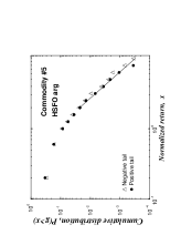
FIG. 2.: Cumulative distributions of positive and negative returns for high-sulphur fuel oil (HSFO arg) [Table I]. The tails of the distributions shown have power law decays with an exponent $\alpha_{5}=2.6\pm 0.3$ for the negative tail and $\alpha_{5}=2.9\pm 0.06$ for the positive tail, where the exponents and the error bars are estimated by Hill’s method  [16].

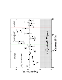
FIG. 3.: (a) Exponents $\alpha_{i}$ of the negative tail and (b) the positive tail, where $i=1,2,..,29$ indexes the 29 commodities analyzed [Table I]. We employ Hill’s method [16] to estimate the exponent $\alpha_{i}$ of each probability distribution in the range $x\geq x_{\rm cutoff}$ where we choose $x_{\rm cutoff}=2$. The dashed lines show the average values $\alpha=(\sum_{i=1}^{29}\alpha_{i})/29$ . Shaded regions indicate the range of Lévy stable exponents, $\alpha<2$.

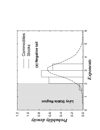
FIG. 4.: Probability density function of (a) the negative tail exponents and (b) the positive tail exponents evaluated for the 7128 stocks and the 29 commodities analyzed. Observe that for both stocks and commodities the mean exponent is around 3.0, outside the Lévy stable region $0<\alpha<2$.

FIG. 5.: (a) Autocorrelation function averaged over all 29 commodities. The autocorrelation function displays an exponential decay with a decay constant of 2.3 days (see inset). (b) The fluctuations $F(n)$ of returns $g_{i}$ and absolute value of returns $|g_{i}|$ averaged over all 29 commodities. The plot for $g_{i}$ is consistent with the exponential decay of Fig. 5(a). The exponent of $\hat{\alpha}=0.73\pm 0.05$ for $|g_{i}|$ implies long-range power law correlation, a feature also seen for stock markets where $\hat{\alpha}\approx 0.8$ [1].

REFERENCES

- [1] P. Gopikrishnan et al. Eur. Phys. J. B 3, 139 (1998); Y. Liu et al. Phys. Rev. E 60, 1390 (1999); V. Plerou et al. Phys. Rev. E 60, 6519 (1999).
- [2] R. N. Mantegna and H. E. Stanley, Nature 376, 46 (1995); P. Gopikrishnan et al. Phys. Rev. E 60, 5305 (1999).
- [3] M. M. Dacorogna, U. A. Müller, R. J. Nagler, R. B. Olsen, and O. V. Pictet, J. Int’l Money and Finance 12, 413 (1993).
- [4] G. Weisbuch, A. Kirman, D. Herreiner, Econ J. 463, 411 (2000); J. P. Nadal, G. Weisbuch, O. Chenevez and A. Kirman, in Advances in Self-Organization and Evolutionary Economics, edited by J. Lesourne and A. Orlian (Economica, London, 1998), p. 149
- [5] For stock markets it is seen that the autocorrelation function decays exponentially to the noise level within a time scale of 4 minutes [1, 2].
- [6] T. Lux, Applied Financial Economics 6, 463 (1996).
- [7] A. Allison and D. Abbott, Unsolved Problems of Noise, edited by D. Abbott and L. Kish (AIP proceedings, Melville, New York, 2000).
- [8] U A. Müller, M. M. Dacorogna, R. B. Olsen, O. V. Pictet, M. Schwarz, and C. Morgenegg, J. Banking and Finance 14, 1189 (1995).
- [9] B. B. Mandelbrot, J. Business 36, 394 (1963).
- [10] W. Working, Wheat Studies 9, 187 (1933).
- [11] W. Working, Wheat Studies of the Stanford Food Institute 2, 75 (1934).
- [12] R. Weron, Physica A 285, 127 (2000).
- [13] B. M. Roehner, Eur. Phys. J. B 8, 151 (1999).
- [14] B. M. Roehner, Eur. Phys. J. B 13, 175 (2000).
- [15] See http://www.platts.com and http://finance.yahoo.com
- [16] B. M. Hill, Ann. Stat. 3, 1163 (1975).
- [17] If we assume that all 29 commodities follow the same distribution then we can aggregate the data, in this way we find for the positive and for the negative tail.
- [18] See http://www.crsp.com
- [19] C. K. Peng, S. V. Buldyrev, S. Havlin, M. Simons, H. E. Stanley, A. L. Goldberger, Phys. Rev. E 49, 1685 (1994).