The spin-$\frac{1}{2}$ Heisenberg antiferromagnet on a 1/7-depleted triangular lattice: Ground-state properties

Abstract

A linear spin-wave approach, a variational method and exact diagonlization are used to investigate the magnetic long-range order (LRO) of the spin-$\frac{1}{2}$ Heisenberg antiferromagnet on a two-dimensional 1/7-depleted triangular (maple leaf) lattice consisting of triangles and hexagons only. This lattice has $z=5$ nearest neighbors and its coordination number $z$ is therefore between those of the triangular ($z=6$) and the kagomé ($z=4$) lattices. Calculating spin-spin correlations, sublattice magnetization, spin stiffness, spin-wave velocity and spin gap we find that the classical 6-sublattice LRO is strongly renormalized by quantum fluctuations, however, remains stable also in the quantum model.

I Introduction

The properties of low-dimensional antiferromagnetic spin systems have been subject of many studies in recent years. A lot of activity in this area was stimulated by the possible connection of such systems with the phenomenon of high-temperature superconductivity. But, the rather unusual properties of quantum magnets deserve study on their own to gain a deeper understanding of these quantum many-body systems, especially at low temperatures. One of the main issues studied is the presence of long-range order (LRO) in the ground state of two-dimensional spin-$\frac{1}{2}$ Heisenberg antiferromagnets (HAF), described by the Hamiltonian

$$H=J\sum_{<i,j>}{\bf S}_{i}\cdot{\bf S}_{j}$$ (1)

on different two-dimensional lattices. The sum runs over all pairs of nearest neighbors on the lattice under consideration and the coupling $J$ is positive.

It is rather well established that LRO is present in the ground state of the spin-$\frac{1}{2}$ HAF on bipartite lattices (square Man , honeycombDea ; Mat , 1/5-depleted squareTro ; Ma , square-hexagonal-dodecagonalToRi ) and, contrary to some early worksAnd ; Faz , also on triangular latticeBer1 ; Ber2 ; Cap . Those results were obtained and confirmed by different methods: exact diagonalization (ED), Monte-Carlo simulations, spin-wave and variational approaches, series expansions and others. It is also worth noticing that recent experiments show that real systems can be modeled by spin-$\frac{1}{2}$ Heisenberg antiferromagnets with different couplings on some uniform Kag ; Col and even depleted lattices Tan .

A regular depletion of the triangular lattice by a factor of 1/4 yields the kagomé lattice with coordination number $z$=4. Contrary to the triangular lattice the ground state of the spin-$\frac{1}{2}$ HAF on the kagomé lattice is most likely a spin liquid.Lech ; Wal However, the kagomé lattice is not the only regularly depleted triangular lattice. As recently has been pointed out by Betts Betts a regular depletion of the triangular lattice by a factor of 1/7 yields another translationally invariant lattice. The coordination number of this lattice is $z=5$ and lies between those of the triangular ($z=6$) and the kagomé ($z=4$) lattices. According to Betts we will call this lattice in what follows the maple leaf lattice. Since, in general, magnetic order is weakened by frustration and low coordination number $z$, it is natural to ask whether the magnetic LRO, present for the HAF on triangular lattice but absent for the HAF on kagomé lattice, will survive this 1/7 depletion of the triangular lattice or not. In this paper we will study this problem using several analytical and numerical methods to calculate the ground state of model (1).

The paper is organized as follows: In Section II we briefly illustrate the geometrical properties of the lattice and the classical magnetic ground state, in Section III exact diagonalization data for finite lattices of $N=18$ and $36$ spins are presented and compared with approximate data (spin-wave and variational), in Section IV a linear spin-wave approach to this problem is presented, results of variational calculations are described in Section V, and the summary is given in Section VI.

II Geometry of the lattice and the classical ground state

The maple leaf lattice is shown in Fig.1. It belongs to the class of uniform tilings in 2D built by a periodic array of regular polygons. In each of the equivalent sites 4 triangles and one hexagon meet. The maple leaf lattice has no reflection symmetry. Its unit cell (marked by dashed lines in Fig.1) consists of 6 sites and 15 bonds. The underlying Bravais lattice is a triangular one. The basis vectors are ${\bf r}_{1}=b\sqrt{7}\left[\sqrt{3}/2,1/2\right]$ and ${\bf r}_{2}=b\sqrt{7}\left[0,1\right]$, where $b$ is the distance between neigboring sites. More information can be found in Ref. Betts .

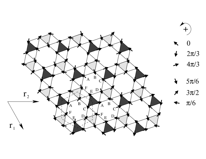
Figure 1: 1/7-depleted triangular (maple leaf) lattice. The geometrical unit cell containing six spins is marked by the dashed lines. This lattice may be split into 6 equivalent triangular sublattices A,B,C, …, F. The classical ground state is represented by arrows.

The ground state of a classical spin system on such a lattice forms the starting point for the calculation of the ground state properties of the quantum HAF within the spin-wave method (section IV) and variational method (section V). As reported previouslySch , this ground state is a non-collinear (canted) planar state with six sublattices. It can be characterized as follows: We denote the position of $i$-th hexagon (unit cell) by lattice vector ${\bf R}_{i}$ and label the sites in the unit cell by the running index $n=1,...,6$. Then we can write

$${\bf S}_{in}=s\left(\cos\left(\phi_{n}+{\bf Q}\cdot{\bf R}_{i}\right){\bf e}_{1}+\sin\left(\phi_{n}+{\bf Q}\cdot{\bf R}_{i}\right){\bf e}_{2}\right),$$ (2)

where ${\bf e}_{1}$ and ${\bf e}_{2}$ are arbitrary orthogonal unit vectors. For the angles $\phi_{n}$ we have
$\phi_{n}-\phi_{m}=\pm\alpha$ for nearest neighbors on the hexagon within the unit cell. The corresponding product of two spin vectors reads ${\bf S}_{in}\cdot{\bf S}_{mj}=s^{2}\cos\left(\phi_{n}-\phi_{m}+{\bf Q}\cdot\left({\bf R}_{i}-{\bf R}_{j}\right)\right).$ The classical ground state corresponds to two sets of ’wave vector’ Q and pitch angle $\alpha=\phi_{B}-\phi_{A}$, namely ${\bf Q}_{1}=2\pi\frac{1}{b\sqrt{7}}\left[\frac{1}{\sqrt{3}},\frac{1}{3}\right],\alpha_{1}=-\frac{5}{6}\pi\;$ and $\;{\bf Q}_{2}=2\pi\frac{1}{b\sqrt{7}}\left[0,\frac{2}{3}\right],\alpha_{2}=\frac{5}{6}\pi$. This is a kind of trivial degeneracy which one can also encounter in the system of classical spins residing on the triangular lattice. The classical ground state energy is given by

$$E_{0}^{cl}=-\frac{J}{2}Ns^{2}\left(1+\sqrt{3}\right),$$ (3)

where $N$ is the number of sites. For spin $s=\frac{1}{2}$ and $J=1$, we have the energy per bond $E/bond=-(\sqrt{3}+1)/20\approx-0.137$. Notice that for the HAF on triangular and kagomé lattices $E/bond=-0.125$.

The classical ground state for $\;{\bf Q}={\bf Q}_{2}$ is illustrated in Fig.1. One has six triangular sublattices A,B,…,F. The classical spins attached to the sublattices are rotated from one unit cell to the next one by the angle $-\frac{2}{3}\pi$ in the direction of basis vector ${\bf r}_{1}$ and by the angle $\frac{2}{3}\pi$ in the direction of ${\bf r}_{2}$. The angle between the nearest spins on each hexagon is $\frac{5}{6}\pi$ or $-\frac{5}{6}\pi$ and three spins residing on each equilateral triangle (marked by light and dark grey in Fig.1) coupled to three nearest hexagons form a $120^{\circ}$-structure.

Though the classical ground state of the maple leaf lattice is more complex than that of the triangular lattice both are Néel states, however, with more than two sublattices. At the same time the classical ground state properties of the kagomé lattice exhibiting a nontrivial ground state degeneracy are completely different.

III The exact diagonalization

We used the Lanczos algorithm to calculate the lowest eigenvalue and the corresponding eigenstate of finite lattices of $N=12,18,24,30,36$ sites. This method has sucessfully applied to finite triangular and kagomé lattices. Unfortunatly, for the maple leaf lattice only the lattice with $N=18$ has the complete p6-symmetry of the infinite lattice and only multiples of 18 fit to the symmetry of the classical ground state. Hence we focus on the lattices with $N=18$ and $N=36$ shown in Fig.2. To reduce the Hilbert space of the Hamiltonian we use all possible translational and point symmetries as well as spin reflection. The number of symmetries of the $N=36$ lattice is lower than that of corresponding $N=36$ triangular and kagomé lattices and the number of symmetrized basis in the $S_{tot}^{z}=0$ ground state sector is 378,221,361. The ground state energy per bond for $N=18$ is $E_{0}/bond=-0.2190042J$ and for $N=36$ is $E_{0}/bond=-0.2155890J$. The spin-spin correlation functions for $N=18$ are collected in Table 1 and for $N=36$ in Table 2 where they are compared to those obtained within spin-wave and variational approach (see below). In the fully symmetric $N=18$ lattice we have three different nearest-neighbor (NN) correlations. The NN correlation $\langle{\bf S}_{0}{\bf S}_{1}\rangle=-0.186299$ (solid lines in Fig.2) corresponds to the classical $120^{\circ}$ bond (see Fig.1); the respective averaged value for $N=36$ is $-0.177732$. Both values are very close to the NN correlation for the triangular lattice. The NN correlation along a hexagon (dashed lines in Fig.2) is strong $\langle{\bf S}_{0}{\bf S}_{2}\rangle=-0.366673$ (the respective averaged value for $N=36$ is $-0.365555$) and is close to the NN correlation of the honeycomb lattice. Finally, the NN correlation corresponding to a classical $90^{\circ}$ bond (dotted lines in Fig.2) is very small $\langle{\bf S}_{0}{\bf S}_{11}\rangle=0.010923$ (the respective averaged value for $N=36$ is $-0.037491$). Hence the NN correlations of the quantum system reflect very well the classical ground state.

The finite-system order parameter corresponding to the classical ground state is the structure factor (square of sublattice magnetization)

$$m^{2}=\frac{6}{N^{2}}\sum_{i,j=1}^{N/6}\sum_{n=1}^{6}e^{i{\bf Q}({\bf R}_{i}-{\bf R}_{j})}\langle{\bf S}_{in}{\bf S}_{jn}\rangle.$$ (4)

The values for $N=18$ and $36$ are listed in Table 4. A finite-size scaling of the order parameter with only two points seems to be not reasonable, however, doing so with a $N^{-1/2}$ scaling we obtain a finite value of $m^{2}$ for $N\to\infty$.

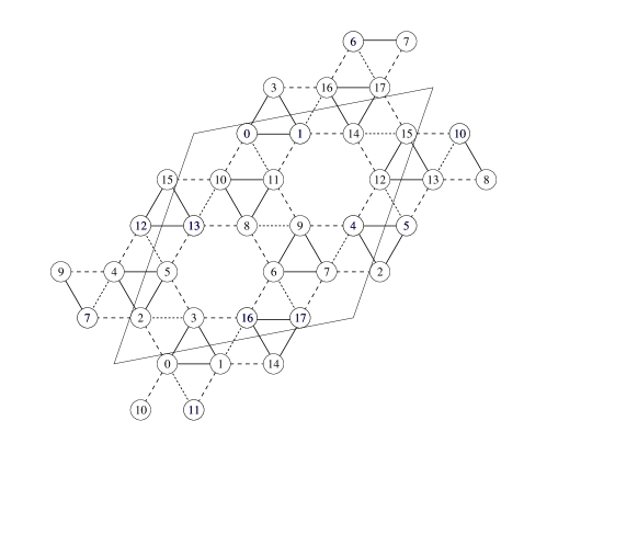
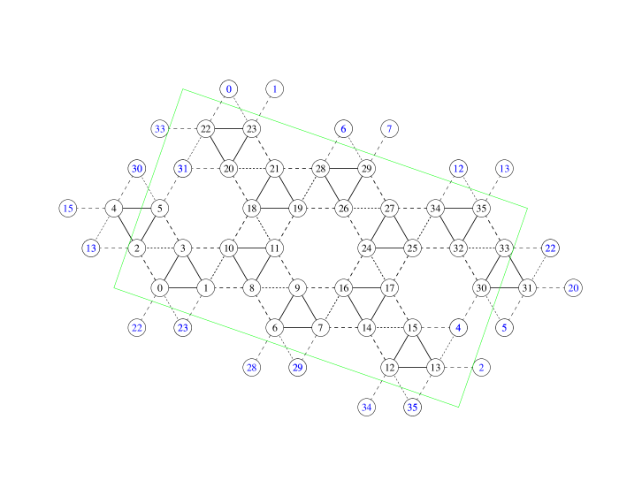
Figure 2: Finite 1/7-depleted triangular (maple leaf) lattices with $N=18$ and $N=36$ sites.

Figure 3: The dependence of the spin-spin correlation on the Euclidean distance for the HAF on the finite maple leaf lattice with $N=36$ sites shown in Fig.2. (a) comparison between exact diagonalization results for different lattices. Data for kagomé are taken from Ref. Leu . (b) Comparison between exact diagonalization, spin-wave and variational results. The lines are guide for the eyes.

A better way is the direct comparison of the spin-spin correlations with those for the HAF on triangular and kagomé latticesLeu . For the presentation of the data we have to take into account that in the classical six-sublattice Néel state we have for instance spins with a relative angle of $90^{\circ}$ leading to special correlations being zero for arbitrary distances. Therefore we consider as a measure for magnetic order the strongest correlations. Consequently we present in Fig.3a the maximal absolute correlations $|\langle{\bf S}_{0}{\bf S}_{r}\rangle|$ versus Euclidian distance $r$. As expected we have very rapidly decaying correlations for the disordered kagomé case, whereas the correlations for the Néel ordered triangular lattice are much stronger for larger distances. Though the correlations for the maple leaf lattices are smaller than those of the triangular lattice they are significantly stronger than those of the kagomé lattice and a kind of saturation for larger distances is suggested.

The results for the spin-spin correlation are used to estimate the quality of the spin-wave and variational method used below by comparing the exact and approximate correlations $|\langle{\bf S}_{0}{\bf S}_{r}\rangle|$ for the finite lattice of $N=36$ (Fig.3b).

IV The linear spin-wave approach

Taking into account that we have six sites in the geometrical unit cell the appropriate representation of the general Hamiltonian (1) reads

$$H=J\sum_{<i,j;n,m>}{\bf S}_{in}\cdot{\bf S}_{jm}$$ (5)

where $i,j$ label the unit cells and $n,m=1,\ldots,6$ the different sites in one unit cell. Of course, the sum runs over neighboring sites, only. The linear spin-wave theory (LSWT) is carried out as usual. However, we need at least six different types of magnons, which makes the calculation more ambitious than for the triangular or the kagomé lattice. We use as quantization axis the local orientation of the spins in the classical ground state. Performing the linear Holstein-Primakoff transformation the scalar product ${\bf S}_{in}\cdot{\bf S}_{jm}$ in (5)) is replaced by the bosonic quadratic form

$${\bf S}_{in}{\bf S}_{jm} \rightarrow s^{2}\cos\Theta_{nm}^{ij}-s\cos\Theta_{nm}^{ij}\left(a_{ni}^{+}a_{ni}+a_{mj}^{+}a_{mj}\right)$$ (6)

$$+ s\left(\cos\Theta_{nm}^{ij}-1\right)\left(a_{ni}^{+}a_{mj}^{+}+a_{ni}a_{mj}\right)/2$$

$$+ s\left(\cos\Theta_{nm}^{ij}+1\right)\left(a_{ni}^{+}a_{mj}+a_{ni}a_{mj}^{+}\right)/2,$$

where $n,m=1,\ldots,6$ label the different magnons in a unit cell $i$. $\Theta_{nm}^{ij}$ represents the angle between the respective classical spin vectors. After transforming the Hamiltonian (5) into the ${\bf k}$-space one obtains

$$H=-\frac{J}{2}Ns^{2}\left(1+\sqrt{3}\right)+Js\sum_{{\bf k}}H_{\bf k},$$ (7)

where

$$H_{{\bf k}} = \left(1+\sqrt{3}\right)\left(a_{1{\bf k}}^{+}a_{1{\bf k}}+a_{2{\bf k}}^{+}a_{2{\bf k}}+a_{3{\bf k}}^{+}a_{3{\bf k}}+a_{4{\bf k}}^{+}a_{4{\bf k}}+a_{5{\bf k}}^{+}a_{5{\bf k}}+a_{6{\bf k}}^{+}a_{6{\bf k}}\right)$$ (8)

$$- \frac{\left(2+\sqrt{3}\right)}{4}\gamma_{1{\bf k}}^{\ast}\left(a_{2{\bf k}}^{+}a_{3-{\bf k}}^{+}+a_{6{\bf k}}^{+}a_{5-{\bf k}}^{+}\right)-\frac{\left(2+\sqrt{3}\right)}{4}\gamma_{1{\bf k}}\left(a_{2{\bf k}}a_{3-{\bf k}}+a_{6{\bf k}}a_{5-{\bf k}}\right)$$

$$+ \frac{\left(2-\sqrt{3}\right)}{4}\gamma_{1{\bf k}}^{\ast}\left(a_{2{\bf k}}^{+}a_{3{\bf k}}+a_{6{\bf k}}^{+}a_{5{\bf k}}\right)+\frac{\left(2-\sqrt{3}\right)}{4}\gamma_{1{\bf k}}\left(a_{2{\bf k}}a_{3{\bf k}}^{+}+a_{6{\bf k}}a_{5{\bf k}}^{+}\right)$$

$$- \frac{\left(2+\sqrt{3}\right)}{4}\gamma_{2{\bf k}}^{\ast}\left(a_{4{\bf k}}^{+}a_{5-{\bf k}}^{+}+a_{2{\bf k}}^{+}a_{1-{\bf k}}^{+}\right)-\frac{\left(2+\sqrt{3}\right)}{4}\gamma_{2{\bf k}}\left(a_{4{\bf k}}a_{5-{\bf k}}+a_{2{\bf k}}a_{1-{\bf k}}\right)$$

$$+ \frac{\left(2-\sqrt{3}\right)}{4}\gamma_{2{\bf k}}^{\ast}\left(a_{4{\bf k}}^{+}a_{5{\bf k}}+a_{2{\bf k}}^{+}a_{1{\bf k}}\right)+\frac{\left(2-\sqrt{3}\right)}{4}\gamma_{2{\bf k}}\left(a_{4{\bf k}}a_{5{\bf k}}^{+}+a_{2{\bf k}}a_{1{\bf k}}^{+}\right)$$

$$- \frac{\left(2+\sqrt{3}\right)}{4}\gamma_{3{\bf k}}^{\ast}\left(a_{6{\bf k}}^{+}a_{1-{\bf k}}^{+}+a_{4{\bf k}}^{+}a_{3-{\bf k}}^{+}\right)-\frac{\left(2+\sqrt{3}\right)}{4}\gamma_{3{\bf k}}\left(a_{6{\bf k}}a_{1-{\bf k}}+a_{4{\bf k}}a_{3-{\bf k}}\right)$$

$$+ \frac{\left(2-\sqrt{3}\right)}{4}\gamma_{3{\bf k}}^{\ast}\left(a_{6{\bf k}}^{+}a_{1{\bf k}}+a_{4{\bf k}}^{+}a_{3{\bf k}}\right)+\frac{\left(2-\sqrt{3}\right)}{4}\gamma_{3{\bf k}}\left(a_{6{\bf k}}a_{1{\bf k}}^{+}+a_{4{\bf k}}a_{3{\bf k}}^{+}\right)$$

$$- \frac{3}{4}\gamma_{1{\bf k}}^{\ast}\left(a_{4{\bf k}}^{+}a_{6-{\bf k}}^{+}+a_{3{\bf k}}^{+}a_{1-{\bf k}}^{+}\right)-\frac{3}{4}\gamma_{1{\bf k}}\left(a_{4{\bf k}}a_{6-{\bf k}}+a_{3{\bf k}}a_{1-{\bf k}}\right)$$

$$+ \frac{1}{4}\gamma_{1{\bf k}}^{\ast}\left(a_{4{\bf k}}^{+}a_{6{\bf k}}+a_{3{\bf k}}^{+}a_{1{\bf k}}\right)+\frac{1}{4}\gamma_{1{\bf k}}\left(a_{4{\bf k}}a_{6{\bf k}}^{+}+a_{3{\bf k}}a_{1{\bf k}}^{+}\right)$$

$$- \frac{3}{4}\gamma_{2{\bf k}}^{\ast}\left(a_{6{\bf k}}^{+}a_{2-{\bf k}}^{+}+a_{5{\bf k}}^{+}a_{3-{\bf k}}^{+}\right)-\frac{3}{4}\gamma_{2{\bf k}}\left(a_{6{\bf k}}a_{2-{\bf k}}+a_{5{\bf k}}a_{3-{\bf k}}\right)$$

$$+ \frac{1}{4}\gamma_{2{\bf k}}^{\ast}\left(a_{6{\bf k}}^{+}a_{2{\bf k}}+a_{5{\bf k}}^{+}a_{3{\bf k}}\right)+\frac{1}{4}\gamma_{2{\bf k}}\left(a_{6{\bf k}}a_{2{\bf k}}^{+}+a_{5{\bf k}}a_{3{\bf k}}^{+}\right)$$

$$- \frac{3}{4}\gamma_{3{\bf k}}^{\ast}\left(a_{2{\bf k}}^{+}a_{4-{\bf k}}^{+}+a_{1{\bf k}}^{+}a_{5-{\bf k}}^{+}\right)-\frac{3}{4}\gamma_{3{\bf k}}\left(a_{2{\bf k}}a_{4-{\bf k}}+a_{1{\bf k}}a_{5-{\bf k}}\right)$$

$$+ \frac{1}{4}\gamma_{3{\bf k}}^{\ast}\left(a_{2{\bf k}}^{+}a_{4{\bf k}}+a_{1{\bf k}}^{+}a_{5{\bf k}}\right)+\frac{1}{4}\gamma_{3{\bf k}}\left(a_{2{\bf k}}a_{4{\bf k}}^{+}+a_{1{\bf k}}a_{5{\bf k}}^{+}\right)$$

$$- \frac{1}{2}\gamma_{1{\bf k}}^{\ast}\left(a_{5{\bf k}}^{+}a_{2-{\bf k}}^{+}-a_{5{\bf k}}^{+}a_{2{\bf k}}\right)-\frac{1}{2}\gamma_{1{\bf k}}\left(a_{5{\bf k}}a_{2-{\bf k}}-a_{5{\bf k}}a_{2{\bf k}}^{+}\right)$$

$$- \frac{1}{2}\gamma_{2{\bf k}}^{\ast}\left(a_{1{\bf k}}^{+}a_{4-{\bf k}}^{+}-a_{1{\bf k}}^{+}a_{4{\bf k}}\right)-\frac{1}{2}\gamma_{2{\bf k}}\left(a_{1{\bf k}}a_{4-{\bf k}}-a_{1{\bf k}}a_{4{\bf k}}^{+}\right)$$

$$- \frac{1}{2}\gamma_{3{\bf k}}^{\ast}\left(a_{3{\bf k}}^{+}a_{6-{\bf k}}^{+}-a_{3{\bf k}}^{+}a_{6{\bf k}}\right)-\frac{1}{2}\gamma_{3{\bf k}}\left(a_{3{\bf k}}a_{6-{\bf k}}-a_{3{\bf k}}a_{6{\bf k}}^{+}\right)$$

with $\gamma_{{\bf k}n}=\exp(i{\bf k}{\bf q}_{n})$, ${\bf q}_{1}=b/\sqrt{28}\left(-\sqrt{3},5\right)$, ${\bf q}_{2}=b/\sqrt{28}\left(-2\sqrt{3},-4\right)$, ${\bf q}_{3}=b/\sqrt{28}\left(3\sqrt{3},-1\right)$ and with $b$ being the distance between two neighboring spins. This Hamiltonian can be diagonalized by the Bogoljubov transformation

$$a_{n{\bf k}}=\sum_{m=1}^{6}u_{n{\bf k}}\alpha_{m{\bf k}}+v_{n-{\bf k}}^{\ast}\alpha_{m-{\bf k}}^{+}.$$ (9)

The new bosonic operators $\alpha_{m{\bf k}}$ describe the normal modes $\omega_{m{\bf k}}$. In order to determine them and the Bogoljubov coefficients one has to solve the following equations

$$\left[\alpha_{m{\bf k}},H\right]_{-}=\omega_{m{\bf k}}\alpha_{m{\bf k}}\quad,\quad\left[\alpha_{m-{\bf k}}^{+},H\right]_{-}=-\omega_{m{\bf k}}\alpha_{m-{\bf k}}^{+}.$$ (10)

The solution gives six different, non-degenerated spin-wave branches — five of them are optical whereas the remaining one is an acoustical branch. The acoustical branch becomes zero in the center (${\bf k}=0$) and at the edges of the Brillouin zone (${\bf k}=\pm{\bf Q}$ with ${\bf Q}=2\pi\frac{1}{b\sqrt{7}}\left[\frac{1}{\sqrt{3}},\frac{1}{3}\right]$). The expansion of the zero modes in the vicinity of those points gives the spin-wave velocities

$$c_{{\bf k}=0} = Jsb\frac{\sqrt{14}\sqrt{39+23\sqrt{3}}}{4\left(2+\sqrt{3}\right)},$$

$$c_{{\bf k}=\pm{\bf Q}} = Jsb\frac{\sqrt{7}\sqrt{407+235\sqrt{3}}}{4\left(7+4\sqrt{3}\right)}.$$ (11)

The acoustical branch of the maple leaf lattice is similar to that of the HAF on the triangular latticeMiy ; Chu , where one has a threefold degenerated acoustical branch being zero for ${\bf k}=0$ and at the edges of the Brilloiun zone $k=\pm{\bf Q}=\pm 2\pi/a\left[1/\sqrt{3},1/3\right]$. The situation for the HAF on the kagomé lattice is completely different. Starting from the so-called classical ${\bf k}=0$ state one obtains three branches, one dispersionsless (flat) mode $\omega_{\bf k}=0$ and two degenerated acoustical branches Har .

In analogy to the triangular latticeChu it can be shown that the zero modes ${\bf k}=0,\pm{\bf Q}$ of the maple leaf lattice describe out-of-plane and in-plane oscillations, respectively. Therefore, we denote $c_{{\bf k}=0}$ as $c_{\parallel}$ and $c_{{\bf k}=\pm{\bf Q}}$ as $c_{\perp}$. Together with the spin-wave velocity the spin stiffness constitutes the fundamental parameters which determine the low-energy dynamics of magnetic systems chakra89 . To calculate the spin stiffness $\rho$ in the leading order $s^{2}$ one can use the hydrodynamic relation $\rho=\chi c^{2}$. The magnetic susceptibilities $\chi_{\parallel}=\chi_{zz}/V$ (out-of-plane) and $\chi_{\perp}=\chi_{xx}/V=\chi_{yy}/V$ (in-plane) can be determined minimizing the classical energy in the limit of a vanishing external field. We find $\chi_{zz}=N/J\left(6+\sqrt{3}\right)$, $\chi_{xx}=\chi_{yy}=2N/3J\left(4+\sqrt{3}\right)$ and $V=7\sqrt{3}Nb^{2}/12$ as the volume of the lattice and from the hydrodynamic relation one obtains

$$\rho_{\parallel}=0.633975Js^{2},\quad\rho_{\perp}=0.211325Js^{2},\quad\rho_{\parallel}/\rho_{\perp}=3\;.$$ (12)

The comparison with the corresponding parameters calculated in the same order in $s$ for the square and the triangular lattice are given in Table 3. We find that the spin stiffness parameters for the maple leaf lattice are lower than the corresponding values of the triangular lattice indicating that the Néel is stronger influenced by quantum fluctuations in the maple leaf lattice than in the triangular one.

The ground state energy $E_{0,N}^{sw}$ is given by

$$E_{0,N}^{sw}=-\frac{J}{2}Ns\left(s+1\right)\left(1+\sqrt{3}\right)+\sum_{{\bf k}}\sum_{m=1}^{6}\omega_{m{\bf k}}/2,$$ (13)

which leads in the thermodynamic limit to an energy per bond

$$e_{0}^{sw}=\left(-0.5464106s^{2}-0.13652065s\right)J.$$ (14)

The sublattice magnetization

$$\left\langle S_{in}^{z}\right\rangle_{N}=\left\langle S^{z}\right\rangle_{N}=s-\frac{6}{N}\sum_{{\bf k}}\left\langle a_{n{\bf k}}^{+}a_{n{\bf k}}\right\rangle$$ (15)

calculated in the thermodynamic limit is

$$\left\langle S^{z}\right\rangle_{\infty}=s-0.346.$$ (16)

A comparison between all those values for HAF on square, triangular and maple leaf lattices is given in Table 3. Obviously, for all these parameters $c$, $\rho$ and $\left\langle S^{z}\right\rangle_{\infty}$ the same tendency is found, namely to be largest for the unfrustrated lattice and to be lowest for the frustrated maple leaf lattice with $z=5$. Notice, that for the kagomé lattice the LSWT yields divergent contributions in the sum over $\bf k$ in $\left(\langle S^{z}\rangle_{N}-s\right)\propto\sum_{{\bf k}}\left\langle a_{n{\bf k}}^{+}a_{n{\bf k}}\right\rangle$ indicating a vanishing sublattice magnetization asakawa .

Finally, we compare the spin-spin correlations $\langle{\bf S}_{0}{\bf S}_{j}\rangle$ (where $j$ runs over all spins in the system) obtained within the LSWT for the finite lattice with $N=36$ shown in Fig.2 with the exact numerical Lanczos data (see Fig.3a and Table 2). One finds a surprisingly good agreement between the approximative LSWT data and the exact Lanczos data. Hence the finding of finite sublattice magnetization obtained within LSWT is supported by the Lanczos data.

V The variational approach

The classical ground state, described in Section II, is the basis for the construction of the variational Huse-Elser HuEl ground state which, expanded in the Ising basis states $\mid\!\alpha\rangle$ of the total spin component $S^{z}=0$ Car ; ToRi , reads

$$\mid\!\!\Psi\rangle=\sum_{\alpha}\,\exp(\frac{1}{2}\tilde{H}_{class}+\frac{1}{2}\tilde{H}_{quant}+\frac{1}{2}\tilde{H}_{frust})\mid\!\alpha\rangle.$$ (17)

The operators $\tilde{H}$ are diagonal in the base $|\alpha\rangle$. The term

$$\tilde{H}_{class}=-i\sum_{j}\phi_{j}S^{z}_{j}$$ (18)

produces a proper ’classical’ phase for a given state $|\alpha\rangle$ in the expansion given by Eq. (17). The sum runs over all spins in the system (i.e. the index $j$ corresponds to a pair $(i,n)$ of indices in Eqs. (4) and (5). $\phi_{j}$ is the angle specified in Fig.1.

The second operator containing variational parameters $K_{jk}$

$$\tilde{H}_{quant}=\sum_{j,k}K_{jk}S^{z}_{j}S^{z}_{k}$$ (19)

provides the amplitude for a given basis state $|\alpha\rangle$ and introduces the quantum corrections to the classical function by taking into account spin-spin correlations. It means that in this approach one starts from the state with a broken rotational symmetry and this is still present during the minimization procedure producing the final symmetry-broken ordered state HuEl ; ToRi .

Finally, the third operator which contains the variational parameter $L_{jkl}$ and the corresponding sign factors $\gamma_{jkl}=\pm 1$

$$\tilde{H}_{frust}=i\sum_{j,k,l}\gamma_{jkl}L_{jkl}S^{z}_{j}S^{z}_{k}S^{z}_{l}$$ (20)

describes an additional possible change of the classical phase due to the quantum fluctuations. Following the ideas of Huse and Elser HuEl we assume that the wave function of the quantum ground state (i.e. $\mid\!\!\Psi\rangle$ from Eq. (17) with all three terms $\tilde{H}_{class}$, $\tilde{H}_{quant}$ and $\tilde{H}_{frust}$) has the same symmetry properties as its classical part (i.e. $\mid\!\!\Psi\rangle$ from Eq. (17) with only $\tilde{H}_{class}$): the sign of the imaginary part of the wave function changes under the rotation $R_{z}(\pi/3)$ by the angle $\pi/3$ whereas remains unchanged under the rotation $R_{z}(2\pi/3)$ by the angle $2\pi/3$ about the center of a hexagon. This transformation determines the ’shape’ of three-spin terms $L_{jkl}$ and the proper sign of $\gamma_{jkl}=\pm 1$ in Eq. (20). Similarly to the triangular lattice HuEl the most simple three-spin terms are ’dog legs’ with $j$ and $l$ being nearest neighbors of $k$. For example, for spin number 5 of the $N=18$ lattice shown in Fig. 2 (top) there exist four such ’interactions’: $L_{3,5,13},L_{3,5,4},L_{2,5,12}$ and $L_{4,5,13}$. Each $L_{ijk}$ is connected with its corresponding $\gamma$ factor, i.e. $L_{3,5,13}\to\gamma_{3,5,13}=\gamma_{EFA}$, $L_{3,5,4}\to\gamma_{3,5,4}=\gamma_{EFD}$, $L_{2,5,12}\to\gamma_{2,5,12}=\gamma_{BFC}$ and $L_{4,5,13}\to\gamma_{4,5,13}=\gamma_{DFA}$, where the letters A,B,C,D,E,F correspond to the 6 equivalent triangular sublattices illustrated in Fig.1. Taking into account that $R_{z}(\pi/3)(ACE)=(BDF)$, $R_{z}(\pi/3)(BDF)=(CEA)$ and $R_{z}(2\pi/3)(ACE)=(CEA)$, $R_{z}(2\pi/3)(BDF)=(DFB)$, i.e., the ’$120^{\circ}$ structure’ ACE (dark triangles in Fig. 1) transforms into ’$120^{\circ}$ structure’ BDF (grey triangles in Fig. 1) under $R_{z}(\pi/3)$ or into itself under $R_{z}(2\pi/3),$ one obtains a proper signs of $\gamma$ factors

$$\gamma_{\alpha\alpha\beta}=-\gamma_{\beta\beta\alpha}.$$ (21)

The index $\alpha\alpha\beta$ means that two (different) spins in the three-spin term belong to the same ’$120^{\circ}$ structure’, the remaining one belongs to the other ’$120^{\circ}$ structure’. Thus, for example, if one puts $\gamma_{BFC}=1$ it follows that $\gamma_{CAD}=-1$ (or $\gamma_{2,5,12}=1$ and $\gamma_{12,13,10}=-1$, see Fig. 2).

How does one choose the variational parameters $K_{jk}$ and $L_{jkl}$ in Eq. (17) for the HAF on the maple leaf lattice? We have applied two criteria: a better choice of parameter space should give a lower value of the ground state energy and, if two energies for different parameter spaces are approximately the same, one should choose the parameter space which leads a lower value of the variance $\langle H^{2}\rangle-\langle H\rangle^{2}$. In order to find an optimal choice of the wave function we have tested some possibilities for the parameter space for the fully symmetrical $N=18$ lattice taking into account the whole $S^{z}=0$ basis in the expansion (17). The best choice found is the following five-parameter space (results for the correlation are collected in Table I): $(K_{hex},K_{tr},K_{others},L_{1},L_{2})$. Spins ’interacting’ via $K_{hex}$ are nearest neighbors lying on a hexagon: hex = AB, BC, CD, …, FA, those ’interacting’ via $K_{tr}$ are nearest neighbors belonging to the $120^{\circ}$ structure: tr = EC, CA, AE or BF, FD, DB; and all remaining nearest neighbors are coupled by $K_{others}$, thus others = BE, BC, EF. Note that there is no long-range variational parameter for pairs of spins not being the nearest neighbors. Moreover, one takes into account only three, from the four existing ’dog leg’ interactions, i.e., ’dog legs’ around a hexagon are absent. For example, in each point F one has $L_{1}=L_{BFC}$ and $L_{2}=L_{EFD}=L_{AFD}$ and $L_{EFA}$ is absent (or correpondingly for spin number 5 in Fig. 2, $L_{1}=L_{2,5,12}$ and $L_{2}=L_{3,5,4}=L_{13,5,4}$ and $L_{3,5,13}$ is absent). All the expectation values of operators reported in the following are calculated for this choice of the variational parameters.

Figure 4: Variational energy per bond for the spin system on the 1/7-depleted triangular (maple leaf) lattice as a function of $N^{-3/2}$.

Having obtained the ground state function one can calculate the expectation values of the operators which characterize the ground state of a given, finite spin system. This can be accomplished by a Monte-Carlo approachHuEl and the finite size scaling HaNi tells how to extrapolate those expectation values to the thermodynamic limit. We have investigated the finite systems of 18, 72, 162, 288 spins with periodic boundary conditions. Note that they have the full symmetry of the maple leaf lattice. The relevant quantities are collected in Table 4 and the finite size analysis is presented in Figs.4 and 5.

Figure 5: Square of sublattice magnetization, $m^{2}$, as a function of $N^{-1/2}$. Circles - values obtained by applying the variational method. Solid line - fit to the circles. Sizes of circles are comparable to the statistical error bars.

The leading term of the finite-size correction of the ground state energy per bond $e$ is $N^{-3/2}$. The data in Table 4 can be fitted to this dependence (see Fig.4) and hence the energy per bond $e_{\infty}$ in the thermodynamic limit is obtained: $e(N)=e_{\infty}+aN^{-3/2}$ with $e_{\infty}=-0.1988(2)J$ and $a=-0.7327(164)J$. This value for $e_{\infty}$ is about 3% higher than the value obtained from spin-wave theory (see Eq. (14)).

In Fig.5 the finite-size extrapolation of the square of sublattice magnetization defined in Eq. (4) is shown. We find $m^{2}(N)=m^{2}_{\infty}+cN^{-1/2}+dN^{-1}$ with $m^{2}_{\infty}=0.0723(10)$, $c=0.0444(18)$ and $d=3.650(60)$ suggesting that the long-range magnetic order persists in the ground state of this spin system. Note, however, that the applied variational ansatz tends to overestimate the magnetic order (see Ref. HuEl and table 2 as well as Fig.3a).

Figure 6: The spin-gap $\Delta=E_{1}-E_{0}$ vs. $1/N$ in units of $J$. $E_{0}$ and $E_{1}$ denote variational energies of the ground state and a first excited state, respectively. Errors result from adding the errors for $E_{0}$ and $E_{1}$.

The variational approach enables us to calculate the spin gap $\Delta=E_{0}-E_{1}$, where $E_{0}$ ($E_{1}$) is the variational energy in the subspace of total $S_{z}=0$ ($S_{z}=1$). This new aspect of the Huse-Elser ansatz was used for the first time in Ref. ToRi to calculate the spin gap for the HAF on the square-hexagonal-dodecagonal lattice. Magnetic LRO is connected with gapless Goldstone modes whereas quantum disorder in the ground state is accompanied by a finite spin gap. Therefore the calculation of $\Delta$ yields an additional argument for or against the existence of magnetic LRO order in the ground state. Fig.6 shows the finite-size extrapolation of the spin gap according to the relation $\Delta(N)=\Delta_{\infty}+dN^{-1}$ with $\Delta_{\infty}=-0.0180(10)J$ and $d=6.3610(34)J$. The negative $\Delta_{\infty}$ is a result of the limitted accuracy of the approximation but nevertheless suggests a zero spin gap. Hence we have an additional indication for the existence of LRO.

VI Summary

In this paper the results of exact diagonalization, linear spin-wave theory and a Huse-Elser like variational investigation for the ground state of the spin-$\frac{1}{2}$ Heisenberg antiferromagnet on a new 1/7-depleted triangular (maple leaf) lattice are presented. The coordination number of this frustrated lattice $z=5$ lies between those of the triangular and the kagomé lattices. Quantum fluctuations and frustration tend to destroy classical magnetic ordering. Their influence becomes the stronger the smaller the coordination number. But contrary to the kagomé lattice with $z=4$ for the maple leaf lattice we find strong arguments that the classical six-sublattice Néel LRO survives the strong quantum fluctuations present in this frustrated quantum magnet. This conclusion is drawn from the calculated values of the spin-spin correlation, sublattice magnetization, spin stiffness, spin-wave velocity as well as the spin gap.

The comparison between exact data and approximate data for the spin-spin correlation on finite lattices gives a surprising well agreement between the linear spin-wave and the exact-digonalization data whereas the variational approach tends to overestimate the strength of correlations.

Finally, we mention that on the passage from the triangular to the 1/7 depleted (maple leaf) lattice (i.e., some interactions $J$ in spin system on triangular lattice are varied from $J=1$ to $J=0$), one would encounter a transition between three-sublattice and six-sublattice Néel LRO which may have interesting features worth to be considered in future.

Acknowledgement

We acknowledge support from the Deutsche Forschungsgemeinschaft (Projects No. Ri 615/10-1 and 436POL 17/5/01) and from the Polish Committee for Scientific Research (Project No. 2 PO3B 046 14). Some of the calculations were performed at the Poznań Supercomputer and Networking Center.

Table 1: The exact values of the spin-spin correlation $\langle{\bf S}_{0}{\bf S}_{j}\rangle$ compared to their variational values for the lattice of $N=18$ sites (see Fig.2).

$j$	exact	variational	$j$	exact	variational
0	0.750000	0.750000	7	0.180027	0.200775
1	-0.186299	-0.180068	8	0.140873	0.162808
2	-0.366673	-0.343444	9	-0.072868	-0.106613
4	0.039003	0.021877	11	0.010923	0.005425
5	0.145098	0.171218	17	-0.174804	-0.183760
6	-0.099672	-0.106613

Table 2: The exact values of the spin-spin correlation $\langle{\bf S}_{0}{\bf S}_{j}\rangle$ compared to their spin-wave and variational values for the lattice of $N=36$ sites (see Fig.2). Statistical errors are given in parentheses.

$j$	exact	spin-wave	variational	$j$	exact	spin-wave	variational
1	-0.1154	-0.16759	-0.1681(90)	19	0.0660	0.05816	0.1574(70)
2	-0.3418	-0.31894	-0.3408(90)	20	0.1458	0.14131	0.1603(60)
3	-0.2008	-0.19143	-0.1703(90)	21	-0.0111	-0.00801	-0.0784(90)
4	0.0618	0.03135	0.0249(70)	22	-0.3929	-0.31878	-0.3395(90)
5	0.1394	0.15200	0.1701(50)	23	-0.0433	-0.06302	0.0027(60)
6	-0.0155	-0.00625	-0.0811(90)	24	0.0434	0.01186	0.1503(70)
7	-0.0243	-0.01525	-0.0788(90)	25	-0.0491	-0.03622	-0.0845(90)
8	0.0089	-0.00304	0.0190(60)	26	-0.0448	-0.02126	-0.1393(90)
10	0.1142	0.12745	0.1546(60)	28	0.0034	-0.01380	0.0089(60)
11	-0.0493	-0.04012	-0.1470(90)	29	0.0298	0.01152	0.1249(70)
12	-0.0155	-0.00625	-0.0832(70)	30	-0.1059	-0.09804	-0.0990(90)
13	0.1488	0.12892	0.1960(50)	31	-0.0740	-0.06787	-0.0939(80)
14	0.0327	0.01839	0.1261(80)	32	0.0387	0.02060	0.0156(70)
15	-0.0797	-0.06993	-0.0946(80)	33	0.1785	0.15290	0.1997(50)
16	-0.0500	-0.03038	-0.1407(90)	34	0.0501	0.04121	0.1313(70)
17	0.0390	0.02791	0.0151(60)	35	-0.1561	-0.11596	-0.1716(90)
18	-0.1059	-0.09804	-0.0992(90)

Table 3: Comparison of the LSWT results for the spin-wave velocities, spin stiffness parameters and sublattice magnetization for the square anderson ; weihong , the triangularChu ; Miy and the maple leaf lattice ($J=1$, $b=1$ and $s=1/2$).

lattice	$c_{\parallel}$	$c_{\perp}$	$\rho_{\parallel}$	$\rho_{\perp}$	$\left\langle S^{z}\right\rangle_{\infty}$
square	1.4142135	1.4142135	0.25	0.25	0.304
triangular	1.2990381	0.9185586	0.2165063	0.1082532	0.239
maple leaf	1.1127356	0.6774616	0.1584936	0.0528312	0.154

Table 4: The ground state energy per bond $E_{0}/bond$, the square of sublattice magnetization $m^{2}$ and the spin gap for the HAF on finite 1/7-depleted triangular (maple leaf) lattices ($J=1$). For the $N=18$ and the $N=36$ lattice the results of exact diagonalization are also included. In the case of the $N=18$ lattice the variational values were obtained in the whole basis of Ising states, for larger systems the Monte-Carlo method was applied. Statistical errors are given in parentheses.

N		$E_{0}/bond$	$m^{2}$	gap
18	exact	-0.2190	0.2832	0.5452
	variational	-0.2083	0.2855	0.3353
36	exact	-0.2155	0.1534
	variational	-0.2027(1)	0.179(1)	0.146(5)
72		-0.2001(1)	0.128(1)	0.071(7)
162		-0.1991(1)	0.099(1)	0.020(10)
288		-0.1988(1)	0.088(1)	0.005(12)
$\infty$		-0.1988(2)	0.072(1)	-0.019(25)

References

- (1) E. Manousakis, Rev. Mod. Phys. 63, 1 (1991).
- (2) D.M. Deaven, D.S. Rokhsar, Phys. Rev. B 53, 14966 (1996).
- (3) A. Mattsson, P. Fröjdh, T. Einarsson, Phys. Rev. B 49, 3997 (1994).
- (4) M. Troyer, H. Kontani, K. Ueda, Phys. Rev. Lett. bf, 3822 (1996).
- (5) L.O. Manuel, M.I. Micheletti, A.E. Trumper, H.A. Ceccatto, Phys. Rev. B 58, 8490 (1998).
- (6) P. Tomczak, J. Richter, Phys. Rev. B 59, 107 (1999).
- (7) P.W. Anderson, Mater. Res. Bull. 8 153 (1973).
- (8) P. Fazekas, P.W. Anderson, Philos. Mag. 30, 423 (1974).
- (9) B. Bernu, C. Lhuillier, L. Pierre, Phys. Rev. Lett. 69, 2590 (1992).
- (10) B. Bernu, P. Lecheminant, C. Lhuillier, L. Pierre, Phys. Rev. B 50, 10048 (1994).
- (11) L. Capriotti, A.E. Trumper, S. Sorella, Phys. Rev. Lett. 82, 3899 (1999).
- (12) H. Kageyama et al., Phys. Rev. Lett. 82, 3168 (2000).
- (13) R. Coldea, D. A. Tennant, A. M. Tsvelik, Z. Tylczyński, Phys. Rev. Lett. 86 1335 (2001).
- (14) S. Taniguchi et al., J. Phys. Soc. Jpn. 64, 2758 (1995).
- (15) P. Lecheminant, B. Bernu, C. Lhuillier, L. Pierre, P. Sindzingre, Phys. Rev. B 56, 2521 (1997).
- (16) Ch. Waldtmann, H.U. Everts, B. Bernu, C. Lhuillier, P. Sindzingre, P. Lecheminant, L. Pierre, Eur. Phys. J. B 2, 501 (1998).
- (17) D.D.Betts, Proc.N.S.Inst.Sci. 40, 95 (1995).
- (18) P.W. Leung, V. Elser, Phys. Rev. B 47, 5459 (1993).
- (19) J. Schulenburg, J. Richter, D.D. Betts, Acta Phys. Polon. 97, 971 (2000).
- (20) A.C. Chubukov, S. Sachdev, T. Senthil, Nucl. Phys. B 426, 601 (1994); cond-mat/9402006
- (21) S.J. Miyake, J. Phys. Soc. Jpn. 61, 983 (1992).
- (22) A.B. Harris, C. Kallin, A.J. Berlinsky, Phys. Rev. B 45, 2899 (1992).
- (23) S. Chakravarty, B.I. Halperin and D.R.Nelson, Phys. Rev B 39, 2344 (1989).
- (24) P.W.Anderson, Phys. Rev 86, 694 (1952).
- (25) Zheng Weihong and C.Hamer Phys. Rev B 47, 7961 (1993).
- (26) H. Asakawa, M. Suzuki, J. Mod. Phys. B 9, 933, (1995).
- (27) D.A. Huse, V. Elser, Phys. Rev. Lett. 60, 2531 (1988).
- (28) C. E. I. Carneiro, X. J. Kong, R. H. Swendsen, Phys. Rev. B 49, 3303 (1994).
- (29) P. Hasenfratz and F. Niedermayer, Z. Phys. B 92, 91 (1993).