Reptation in the Rubinstein-Duke model: the influence of end-reptons dynamics

Abstract

We investigate the Rubinstein-Duke model for polymer reptation by means of density-matrix renormalization group techniques both in absence and presence of a driving field. In the former case the renewal time $\tau$ and the diffusion coefficient $D$ are calculated for chains up to $N=150$ reptons and their scaling behavior in $N$ is analyzed. Both quantities scale as powers of $N$: $\tau\sim N^{z}$ and $D\sim 1/N^{x}$ with the asymptotic exponents $z=3$ and $x=2$, in agreement with the reptation theory. For an intermediate range of lengths, however, the data are well-fitted by some effective exponents whose values are quite sensitive to the dynamics of the end reptons. We find $2.7<z<3.3$ and $1.8<x<2.1$ for the range of parameters considered and we suggest how to influence the end reptons dynamics in order to bring out such a behavior. At finite and not too small driving field, we observe the onset of the so-called band inversion phenomenon according to which long polymers migrate faster than shorter ones as opposed to the small field dynamics. For chains in the range of 20 reptons we present detailed shapes of the reptating chain as function of the driving field and the end repton dynamics.

I Introduction

The idea of reptation was introduced about thirty years ago by de Gennes [1] in order to explain some dynamical properties of polymer melts of high molecular weight. The dynamics of such systems is strongly influenced by entanglement effects between the long polymer chains. The basic idea of reptation is that each polymer is constrained to move within a topological tube due to the presence of the confining surrounding polymers [2, 3]. Within this tube the polymer performs a snake-like motion and advances in the melt through the diffusion of stored length along its own contour. One focuses thus on the motion of a single test chain, while the rest of the environment is considered frozen, i.e. as formed by a network of fixed obstacles. The reptation theory predicts that the viscosity $\mu$ and longest relaxation time $\tau$ (known as renewal time) scale as $\mu\sim\tau\sim N^{3}$, where $N$ is the length of the chains, while the diffusion constant scales as $D\sim 1/N^{2}$. These results are not far from the experimental findings. Measurements of viscosity of concentrated polymer solutions and melts of different chemical composition and nature are all consistent with a scaling $\mu\sim N^{3.4}$ [4], while for the diffusion constant both $D\sim 1/N^{2}$ [5] and $D\sim 1/N^{2.4}$ [6, 7, 8, 9] have been reported. This discrepancy triggered a substantial effort in order to reconcile theory and experiments.

Another physical situation where reptation occurs is in gel electrophoresis, where charged polymers diffuse through the pores of a gel under the influence of a driving electric field [10]. The gel particles form a frozen network of obstacles in which the polymer moves through the diffusion of stored length. Electrophoresis has important practical applications, for instance in DNA sequencing, since it is a technique which allows to separate polymers according to their length.

The previous examples demonstrate how reptation is an important mechanism for polymer dynamics in different physical situations. A prominent role in understanding the subtle details of the dynamics was played by models defined on the lattice, which besides describing correctly the process at the microscopic level, offer important computational advantages. The aim of this paper is to investigate in detail one of such lattice models, which was originally introduced by Rubinstein [11] and later extended by Duke [12] in order to include the effect of an external driving field. The Rubinstein - Duke (RD) model has been studied in the past using several techniques; there are a limited numbers of exact results available [13, 14, 15] while a rich literature on simulation results on the model exists. The latter have been mostly obtained by Monte Carlo (MC) simulations [11, 12, 16, 17]. MC simulations are tedious for long chains since the renewal time scales as $N^{3}$, thus it is difficult to obtain a small statistical error for large $N$.

In this paper we study the RD model by means of Density Matrix Renormalization Group (DMRG) [18], a technique which has been quite successful in recent years, in particular in application to condensed matter problems as quantum spin chains and low-dimensional strongly correlated systems [19]. Using the formal similarity between the Master equation for reptation and the Schrödinger equation, DMRG also allows to calculate accurately stationary state properties of long reptating chains.

Some of the results reported here, in particular concerning the scaling of the renewal time $\tau$, have been presented before [20]. Here we will give full account of the details of the calculations and present a series of new results concerning reptation in the presence of an electric field. One of the main conclusions of our investigation is that the exponents describing the scaling of $\tau$ and $D$ in the intermediate length region appear to be rather sensitive on the structure of the end repton. We find that, by influencing the end repton dynamics, one has a regime where the effective exponents are considerably lower than the standardly found experimental values. Experiments are suggested, involving polymer architectures not investigated so far, and which ought to confirm our predictions.

This paper is organized as follows: in Sec. II we introduce the RD model, while in Sec. III we briefly outline the basic ideas of DMRG. Sec. IV is dedicated to the properties of reptation in absence of an external field, in particular to the scaling properties of $\tau$ and $D$. Sec. V collects a series of results of reptation in a field, while Sec. VI concludes our paper.

II The Rubinstein - Duke model

In the RD model the polymer is divided into $N$ units, called reptons, which are placed at the sites of a $d$-dimensional hypercubic lattice (see Fig. 1). The number of reptons that each site can accommodate is unlimited and self-avoidance effects are neglected. Each configuration is projected onto an axis along the (body) diagonal of the unit cell and it is identified by the relative coordinates $y_{i}\equiv z_{i+1}-z_{i}$ of neighboring reptons along the chain ($z_{i}$ indicates the projected coordinate of the $i$-th repton). The relative coordinates can take three values $y_{i}=-1,0,1$ and there are thus in total $3^{N-1}$ different configurations for a chain with $N$ reptons.

FIG. 1.: Example of a configuration in the RD model in $d=2$ dimensions. In terms of the relative coordinates projected along the field direction the configuration reads $y=\{1,0,1,1,-1,1,0\}$. A non-zero field ($\varepsilon$) biases the motion of the reptons, which occurs with rates $B=\exp(\varepsilon/2)$ $(B^{-1})$ for moves in the direction (opposite to) the applied field. The arrows indicate the possible moves. Notice that an end repton can stretch to $d$ lattice positions forward and backward in the field (as repton $8$ in the example).

When two or more reptons accumulate at the same lattice site they form a part of stored length, which can then diffuse along the chain. In terms of relative coordinates a segment of stored length corresponds to $y_{i}=0$, therefore allowed moves are interchanges of $0$’s and $1$’s, i.e. $0,\pm 1\leftrightarrow\pm 1,0$. On the contrary, the end reptons of the chain can stretch ($0\to\pm 1$) or retract to the site occupied by the neighboring repton ($\pm 1\to 0$). The dynamics of the chain is fully specified once the rates for the moves are given. A field $\varepsilon$ along the projection axes is introduced so that moves forward and backward in the field occur with rates $B=\exp(\varepsilon/2)$ and $B^{-1}=\exp(-\varepsilon/2)$. In the following we will be interested in both cases $\varepsilon=0$ and $\varepsilon>0$. Notice that when an end repton moves towards an empty lattice site (tube renewal process) it has in total $d$ different possibilities of doing so forward and backward in the field (see Fig. 1), therefore the associated rates are $dB$ and $dB^{-1}$ respectively. On the contrary the end repton can retract by moving to the (unique) site occupied by its neighbor with rate $B$ or $B^{-1}$. Summarizing the possible moves are: (a) stored length diffusion for inner segments, i.e. ($0,\pm 1\leftrightarrow\pm 1,0$) with rates $B$ and $B^{-1}$, (b) contractions for external reptons ($\pm 1\to 0$) with rates $B$ and $B^{-1}$ and (c) stretches for external reptons ($0\to\pm 1$), with rates $dB$ and $dB^{-1}$. Notice that the parameter $d$ enters in the model only at the stretching rates (c). Rather than linking $d$ to the lattice coordination number we interpret it as the ratio between stretching rates and rates associated to moves of inner reptons. This allows to choose any positive values for $d$.

FIG. 2.: (a) In thick line we indicate a test chain moving in an environment of other chains. By modifying its ends, for instance, by attaching molecules of large size one can lower the parameter $d$, as in this way one expects that stretchings of the chain out of the tube will occur to lower rate. (b) The lowering of $d$ would also occur for reptating polymers with short branching ends.

As we will see, a variation of $d$ has some important effects on the corrections to the asymptotic behavior. This regime may turn out to be relevant for the experiments. Moreover it is conceivable that the parameter $d$ could be somewhat modified in an experiment. Figure 2 schematically illustrates a possibility of doing so, namely by attaching to the chain ends some large molecules so that for each chain tube renewal moves would be impeded. The same effects would be possible if the linear chain is modified such as to have branches close to the endpoints (Fig. 2(b)), or an end part stiffer than the rest of the chain (as it could be realized in block copolymers). In both cases we expect that stretches out of the confining tube would be suppressed while chain retractions would not be much impeded.

Once the rates for elementary processes are given, the stationary properties of the system can be found from the solution of the Master equation

$$\frac{dP(y,t)}{dt} = -\sum_{y^{\prime}}H_{yy^{\prime}}P(y^{\prime},t)$$ (1)

in the limit $t\to\infty$. Here $P(y,t)$ indicates the probability of finding the polymer in a configuration $y$ at time $t$ and the matrix $H$ contains the transition rates per unit of time between the different configurations of the chains, as given in the rules discussed above.

III Density matrix renormalization

DMRG was introduced in 1992 by S. White [18] as an efficient algorithm to deal with a quantum hamiltonian for one dimensional systems. It is an iterative basis–truncation method, which allows to approximate eigenvalues and eigenstates, using an optimal basis of size $m$. It is not restricted to quantum system; it has also been successfully applied to a series of problems, ranging from two dimensional classical systems [21] to stochastic processes [22]. The basic common feature of these problems is the formal analogy with the Schrödinger equation for a one dimensional many–body system. DMRG can also be applied to the Master Equation (1) for the reptating chain, albeit with some limitations due to the non–hermitian character of the matrix $H$. In this specific case we start from small chains, for which $H$ can be diagonalized completely, and construct effective matrices representing $H$ for longer chains through truncation of the configurational space followed by an enlargement of the chain. This is done through the construction of a reduced density matrix whose eigenstates provide the optimal basis set, as can be shown rigorously (see Refs. [18, 19] for details). The size $m$ of the basis remains fixed in this process. By enlarging $m$ one checks the convergence of the procedure to the desired accuracy. Hence $m$ is the main control parameter of the method. In the present case we found that $m=27$ is sufficient for small driving fields and we kept up to $m=81$ state for stronger fields.

$H$ is only hermitian for zero driving field. So for a finite driving field one needs to apply the non–hermitian variant of the standard DMRG algorithm [22]. For a non–hermitian matrix $H$ one has to distinguish between the right and left eigenvector belonging to the same eigenvalue. Since $H$ is a stochastic matrix the lowest eigenvalue equals 0 and the corresponding left eigenvector is trivial (see next section). The right eigenvector gives the stationary probability distribution. The next to lowest eigenvalue, the gap $1/\tau$, yields the slowest relaxation time $\tau$ of the decay towards the stationary state. Generally the DMRG method works best when the eigenvalues are well separated. For long chains and stronger driving fields the spectrum of $H$ gets an accumulation of eigenvalues near the zero eigenvalue of the stationary state. This hampers the convergence of the method seriously and enlarging the basis $m$ becomes of little help, while standardly this improves the accuracy substantially. In order to construct the reduced density matrix from the lowest eigenstates one needs to diagonalize the effective matrices $H$ at each DMRG step, we used the so-called Arnoldi method which is known to be particularly stable for non-hermitian problems [23].

IV Zero field properties

In this section we present a series of DMRG results on the scaling behavior as function of the polymer length $N$ of the so-called tube renewal time $\tau(N)$, i.e. of the characteristic time for reptation, and of the diffusion coefficient $D(N)$.

A Tube renewal time

The renewal time, $\tau$, is the typical time of the reptation process, i.e. the time necessary to loose memory of any initial configuration through reptation dynamics. $\tau$ is given by the inverse of the smallest gap of the matrix $H$, which can be seen as follows: Starting from an initial configuration one has, asymptotically for sufficiently long times ($t\to\infty$):

$$|P(t)\rangle=|\phi_{0}\rangle+e^{-t/\tau}|\phi_{1}\rangle+\ldots$$ (2)

where $|\phi_{0}\rangle$ and $|\phi_{1}\rangle$ are eigenstates of the matrix $H$ defined in Eq. (1) with eigenvalues $E_{0}=0$ and $E_{1}=1/\tau$, respectively. The state $|\phi_{0}\rangle$ is the stationary state of the process, while the gap of $H$ corresponds to the inverse relaxation time. Notice that, as the matrix $H$ is symmetric at zero field, $E_{1}$ is always a real number, while for non-Hermitian matrices the eigenvalues may get an imaginary part, which causes a relaxation to equilibrium through damped oscillations.

An important point of which we took advantage in the calculation is the fact that the ground state $|\phi_{0}\rangle$ of the matrix $H$ is known exactly in absence of any driving fields. Since $H$ is stochastic and symmetric (i.e. $\sum_{y^{\prime}}H_{yy^{\prime}}=\sum_{y^{\prime}}H_{y^{\prime}y}=0$), it follows immediately that the stationary state is of the form $\phi_{0}(y)=c$, with $c$ a constant. Instead of applying the DMRG technique directly to the matrix $H$ we applied it to the matrix $H^{\prime}$ defined by:

$$H^{\prime}=H+\Delta|\phi_{0}\rangle\langle\phi_{0}|.$$ (3)

Now if we choose $\Delta>E_{1}$ the lowest eigenvalue of $H^{\prime}$ is equal to $E_{1}$, therefore the problem of calculating the gap of $H$ is reduced to the calculation of the ground state of a new (non-stochastic) matrix $H^{\prime}$. This approach is considerably more advantageous in term of CPU time and memory required for the program (for more details see Ref. [24]).

Figure 3 shows a plot of $\ln\tau(N)$ vs. $\ln N$ for the renewal time as calculated from DMRG methods for various values of the stretching rate $d$ and for lengths up to $N=150$. The data have been shifted along the abscissae axis by an arbitrary constant. We fitted the data by a linear interpolation, as it is mostly done in Monte Carlo simulations and in experiments. The resulting slopes provide estimates of the exponent $z$, which we find to be sensitive to the stretching rate $d$. For $d$ sufficiently large ($d>2$) we find $z\approx 3.3$, in agreement with experiments [4] and previous Monte Carlo simulation results [11, 25]. The value of $z$ decreases when $d$ is decreased. For $d$ sufficiently small ($d\approx 0.1$) we find $z\approx 2.7<3$, which is a regime that has not yet been observed in experiments.

FIG. 3.: Plot of $\ln\tau(N)$ vs. $\ln N$ for various $d$. We report the values of the slope of the data obtained from a linear interpolation.

To shed some more light into these results we considered the effective exponent, i.e. the following quantity:

$$z_{N}=\frac{\ln\tau(N+1)-\ln\tau(N-1)}{\ln(N+1)-\ln(N-1)}\,\,,$$ (4)

which is the discrete derivative of the data in the log-log scale plot. Such quantity probes the local slope (at a given length $N$) of the data of Fig. 3 and provides a better estimate of the finite $N$ corrections to the asymptotic behavior. The calculation of $z_{N}$ requires very accurate data and cannot be easily performed by Monte Carlo simulation results which are typically affected by numerical uncertainties, as these are amplified when taking numerical derivatives. We stress that already in the log-log plot of Fig. 3 the deviation of the data from linearity is noticeable, therefore the values of $z$ given above are just average values and not to be expected as asymptotic ones.

Figure 4 shows a plot of $z_{N}$ for the data given in Fig. 3, plotted as function of $1/\sqrt{N}$. In the thermodynamic limit $N\to\infty$, $z_{N}$ is seen to converge towards $z=3$, in agreement with de Gennes’ theory [1]. Corrections to this asymptotic limit yield $z_{N}>3$ when $N$ is sufficiently large, with deviations towards $z_{N}<3$ for small $d$ and not too large $N$.

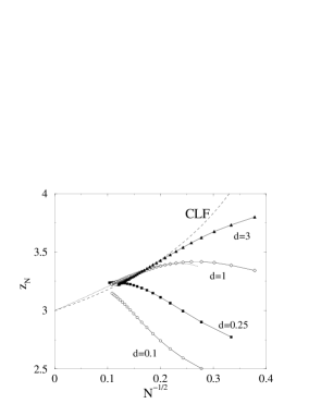
FIG. 4.: Solid lines: Effective exponent $z_{N}$ for various $d$. Dashed line: Corrections due to CLF as predicted by Doi (Eqs. 5 and 6) for the $d=3$ curve. Dot-dashed line: Inclusion of higher order corrections as given by Eq. 8 for the curve $d=1$.

There exist some theoretical predictions for the form of the corrections to the asymptotic behavior of the renewal time [26]. These are based on contour length fluctuations (CLF), i.e. on the idea that the length of the tube fluctuates in time and that this would help accelerating the renewal process. Such fluctuations were not taken into account in the original work of de Gennes, who assumed the tube to have a fixed length. According to CLF theory, thus, $\tau$ scales as [26]

$$\tau(N)\sim N^{3}\left(1-\sqrt{\frac{N_{0}}{N}}\,\,\right)^{2},$$ (5)

with $N_{0}$ a typical length. Substituting this equation into Eq. (4) one obtains:

$$z_{N}^{\rm(CLF)}=3+\frac{\sqrt{N_{0}/N}}{1-\sqrt{N_{0}/N}}\,\,.$$ (6)

which is a monotonically increasing function of $1/\sqrt{N}$. For all lengths in the physical range $N>N_{0}$ one has $z_{N}^{\rm(CLF)}>3$. Eq. (6) is plotted as a dashed line in Fig. 4, where we have chosen $N_{0}=2.3$ in order to obtain the best fit of the DMRG data with $d=3$. This value is consistent with that predicted by the CLF theory [3]. Our results further suggest that the value of $N_{0}$ increases when $d$ is decreased.

While for sufficiently long chains the data apparently merge to the CLF theory given by Eq.(6) higher order corrections appear to be of opposite sign. When $d$ is lowered the latter become particularly strong so that the effective exponent for a certain range of lengths is even smaller than $3$. To our knowledge such an effect has not yet been observed in experiments. Presumably standard polymer mixtures will correspond to $d\gtrsim 1$, which is a regime where an exponent $z\approx 3.4$ is observed [4]. It is conceivable that mixtures with modified architecture, as those illustrated in Fig. 2(b), i.e. long polymers with short branching ends, would correspond to curves at much lower $d$. Experimental results for such systems would be of high interest in order to check the predictions of the RD model in the low $d$ regime.

In order to gain some more insight in the precise form of $\tau(N)$ we considered higher order terms which lead to an expression of the type:

$$\tau(N)\sim N^{3}\left[\left(1-\sqrt{\frac{N_{0}}{N}}\right)^{2}+A\frac{N_{0}}{N}\right]$$ (7)

Recently, Milner and McLeish [27] formulated a more complete theory beyond that of CLF by Doi, using ideas from the theory of stress relaxation for star polymers [28], which to lowest orders in $1/\sqrt{N}$ yields an expression of the type given above. The effective exponent now reads:

$$z_{N}=3+\sqrt{\frac{N_{0}}{N}}\frac{1-(1+A)\sqrt{{N_{0}}/{N}}}{\left(1-\sqrt{{N_{0}}/{N}}\right)^{2}+A{N_{0}}/{N}}$$ (8)

Notice that the CLF expression (Eq. 6) diverges for $N\to N_{0}$, while the previous formula this divergence does not occur. For $N$ not too large the numerator in Eq. (8) may change sign, reproducing features found in the DMRG calculations, i.e. an effective exponent $z<3$. The dot-dashed line of Fig. 4 represents a fit for the $d=1$ case using Eq.(8); we find that the choice $N_{0}=3.6$ and $A=0.44$ fits very well the numerical data for $N>25$, while deviations for shorter chains are clearly visible. We stress that Eq. (8) fits quite well the renewal time data in the cage model [29], which is another lattice model of reptation dynamics [31]. Finally, very recently the effect of constraints release (CR), introduced in the RD model in a self-consistent manner, has been considered [30]. Apart from small quantitative shifts in the effective exponents, the is unchanged.

B Diffusion coefficient

We consider now a similar scaling analysis of the diffusion coefficient $D$. To compute the diffusion constant as function of the chain length we used the Nernst–Einstein relation [14]:

$$D=\lim_{\varepsilon\to 0}\frac{v}{N\varepsilon}.$$ (9)

where $v$ is the drift velocity of the polymer with $N$ reptons and subject to an external field $\varepsilon$. In order to estimate $D(N)$ we considered small fields (down to $\varepsilon\sim 10^{-5}$) and calculated the velocity $v_{i}$ of the $i$-th repton in the stationary state using the formulas given in Section V B. As a check for the accuracy of the procedure we verified that the drift velocity $v_{i}$ is independent on $i$, i.e. the position of the repton along the chain in which it is computed.

TABLE I.: Comparison between diffusion coefficients from exact diagonalization methods, as given in Ref. [17], and as obtained from the calculation of $r(\varepsilon)=v/N\varepsilon$ from the DMRG algorithm with $m=18$ for decreasing $\varepsilon$.

$N$	$r(\varepsilon=10^{-2})$	$r(\varepsilon=10^{-3})$	$r(\varepsilon=10^{-4})$	$DN^{2}$ (Ref. [17])
5	0.864873	0.864907	0.864908	0.864908
7	0.769024	0.769057	0.769057	0.769057
9	0.703975	0.703951	0.703951	0.703951
11	0.657701	0.657550	0.657549	0.657549
13	0.623372	0.623010	0.623006	0.623006
15	0.596975	0.596304	0.596297	0.596297
17	0.576097	0.575007	0.574996	0.574996
19	0.559224	0.557595	0.557580	0.557579

FIG. 5.: Log-log plot of the diffusion constant as function of the chain length for various values of the stretching rate $d$.

In practice we estimated the ratio $r=vN/\varepsilon$ for decreasing $\varepsilon$ until convergence was reached (typically we considered $\varepsilon\approx 10^{-4}-10^{-5}$). Table I shows the numerical values of $r(\varepsilon)$ for various $\varepsilon$ obtained from DMRG with $m=18$ states kept, for short chains, so that they can be compared with the exact diagonalization data shown in the last column. The results for $\varepsilon=10^{-4}$ are in excellent agreement with exact diagonalization data for $DN^{2}$ (from Ref. [17]) reported in the last column, which indicates that the procedure used to extrapolate the diffusion coefficient from the Nernst-Einstein relation (Eq. 9) is correct and reliable.

According to reptation theory the diffusion coefficient for large $N$ should scale as $D(N)\sim 1/N^{2}$ [1]. This results has been also derived rigorously for the RD model where the coefficient of the leading term is also known [32, 15]:

$$D(N)=\frac{1}{(2d+1)N^{2}}$$ (10)

Early experimental results on diffusion coefficients for polymer melts were consistent with a power $-2$ [5], while more recent results suggest that such exponent would be significantly higher [8]. In fact the original measurements consistent with a scaling $1/N^{2}$ raised quite some problems in the past, which was pointing to an inconsistence between the scaling of $D$ and $\tau$ due to the following argument. For a reptating polymer, $D$ and $\tau$ the typical radius of gyration should scale as:

$$R_{g}\sim\sqrt{D\tau}$$ (11)

Now as the polymer obeys gaussian statistics $R_{g}\sim\sqrt{N}$, which implies that, if $\tau\sim N^{3.4}$ then necessarily $D\sim N^{-2.4}$, for the same range of lengths. This argument is however not quite correct in this form since $R_{g}\sim\sqrt{N}$ only asymptotically, thus finite size corrections may affect $D$ and $\tau$ differently, as indeed happens in the RD model.

Figure 5 shows a plot of $\ln D$ as a function of $\ln N$ for various values of the stretching rate $d$. The best fitting parameters $x$ for the scaling $D\sim 1/N^{x}$ are given. As for the diffusion constant the exponent passes the presumed asymptotic value of $2$ for $d=1$ and $d=3$, while $x<2$ for $d=0.5$ and $d=0.1$. Other numerical investigations of the RD and related model yielded $x\approx 2.0$ [11], $x\approx 2.5$ [25], and $x\approx 2.0$ [33]. Again, it is best to analyze the effective exponent

$$x_{N}=-\frac{\ln D(N+1)-\ln D(N-1)}{\ln(N+1)-\ln(N-1)}\,\,,$$ (12)

which is shown in Fig. 6. $x_{N}$ shows a similar behavior as the renewal exponent. However, comparing the same values of $N$ and $d$ in Figs. 4 and 6 one notices that finite $N$ corrections are weaker for the diffusion coefficient. For instance, for $d=3$ and $N^{-1/2}=0.3$ one has $z_{N}\approx 3.8$, while $x_{N}\approx 2.3$. As mentioned above, recent experimental investigation of diffusion coefficient for polymer melts and solutions yielded some different results concerning its scaling behavior. Early measurements of polymer melts yielded $D\sim N^{-2}$ [5], while in concentrated solutions typically $D\sim N^{-2.4}$ [6, 7]. Very recently, however, on hydrogenated polybutadiene concentrated solutions and melts it was found $D\sim N^{-2.4}$ for both cases [9]. A reanalysis of previous experimental results on several different polymers lead to the conclusion $D\sim N^{-2.3}$ [8]. Thus the issue experimentally has not yet fully settled. A theoretical analysis of the contour length fluctuations on the diffusion coefficient was recently performed [34] leading to the expression:

$$D_{\rm CLF}(N)\sim N^{-2}\left(1-\sqrt{\frac{N_{0}}{N}}\right)^{-1}$$ (13)

In Fig. 6 we plotted the corresponding effective exponent, fitted to the $d=3$ results. Again, the numerical results seem to approach the CLF formula only for very long chains, where the effective exponent is already quite close to the asymptotic value. Our results indicate some variation of the effective exponent as function of the parameter $d$. It would be therefore interesting to investigate the scaling of $D$ for the polymer with short branching ends, as those illustrated in Fig. 2(b) in order to test the validity of our predictions at smaller $d$.

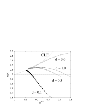
FIG. 6.: Effective exponent $x_{N}$ as defined by Eq. (12) for various $d$. The dotted line is the theoretical prediction from Eq. (13).

Finally we mention that the further order correction terms for the scaling of $D$ have raised recently some debate about the nature of the expansion [16, 15]. The DMRG results, which are accurate enough to investigate the higher orders, clearly show that these results can be very well represented by a series in $1/\sqrt{N}$ [20].

V Reptation in the presence of an electric field

For finite values of $\epsilon$ severe limitations appear preventing us to extend the calculations to the long chains which we were able analyze in the limit $\epsilon\rightarrow 0$. These limitations are intrinsic to the problem and the Arnoldi routine for finding the lowest eigenvalue of the matrix H. For finite $\epsilon$ and longer chains a massive accumulation of small eigenvalues near the ground state eigenvalue starts to emerge. The problem is also present in the straight application of the routine to small chains, for which an exact diagonalization of the matrix $H$ can be performed. For $N>11$ and $\epsilon\geq 1$ the method for finding the lowest eigenvalue is no longer convergent. The DMRG method, described above, yields convergent results up to the chain $N=15$. For smaller fields, $\varepsilon<1$, which is however the most interesting region from the physical viewpoint, the calculation can be extended to somewhat longer chains i.e. $N\approx 30-40$. Neither extension of the truncated basis set, nor the inclusion of more target states is a remedy for the lack of convergence. Despite the intrinsic difficulty of treating long chains, substantial information can be obtained by the analysis of the drift velocity for intermediate chain lengths as function of $\varepsilon$.

A Drift velocity vs. field

In Fig. 7 we have plotted the drift velocity as function of $\epsilon$ for chains up to $N=15$ and stretching ratio $d=1$. The general behavior is a rise turning over into an exponential decay. For small $\varepsilon$ the rise is linear, in agreement with the results presented for the zero field diffusion coefficient. In fact we have calculated the diffusion coefficient as the derivative of the drift velocity with respect to $\varepsilon$ (see Sec. (IV B)). The exponential decay is in accordance with the behavior predicted by Kolomeisky [35]. For large fields the probability distribution narrows down to a single $U$ shaped configuration with equally long arms at both sides of the center of the chain. For odd chains Kolomeisky shows that, in the limit $\varepsilon\to\infty$ [35]

$$v\sim\exp\left(\frac{2-N}{2}\varepsilon\right)$$ (14)

For the chains up to $N=7$ we could confirm this behavior (see inset of Fig. 7), but for the longer chains one would have to go to larger values of $\epsilon$ than can be handled with the Arnoldi method to see the asymptotic behavior. Generally the curves are a compromise between two tendencies: the expression for the drift grows with the field but the probability on a configuration shifts towards configurations with the least velocity. With increasing $\epsilon$ initially the first effect dominates but gradually the second effect overrules the first.

FIG. 7.: The velocities as a function of an electric field for chains of different lengths for $d=1$. Inset: $\ln v$ vs. $\varepsilon$ for $N=7$; the asymptotic behavior is consistent with the prediction from Eq.(14), shown as a dashed line.

We have also investigated the behavior of the velocity as function of the stretching ratio $d$. In Fig. 8 we have plotted the various curves for chain length $N=7$ for $d$ ranging from $0.05$ to $3.25$. We see that the overall velocity becomes small for small $d$ which is simply a sign of slowing down due to the slowed down motion of the end reptons. For the higher values of $d$ we see again a decrease in the drift velocity, which is explained by stretching of the chain as we will see.

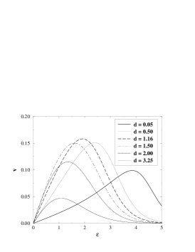
FIG. 8.: The velocities as a function of an electric field for different $d$. The number of reptons is fixed at $N=7$.

A closer inspection of the curves $v$ vs. $\varepsilon$ in the interval $0<\varepsilon\leq 1$ for the longer chains shows a definite deviation of the linear rise to larger values of the drift velocity. This interesting intermediate regime was also investigated by Barkema et al. [16] by means of Monte Carlo simulations. They propose to describe the drift velocity in this region by the phenomenological crossover expression

$$v(\epsilon,N)\simeq\frac{\epsilon}{(2d+1)N}[1+A(\epsilon N)^{2})]^{\frac{1}{2}}$$ (15)

which seems to fit quite well the Monte Carlo data [36]. Thus in the regime where $\epsilon$ is small but the combination $\epsilon N$ of order unity, the drift velocity becomes independent of $N$ (band collapse) and quadratically dependent on $\epsilon$.

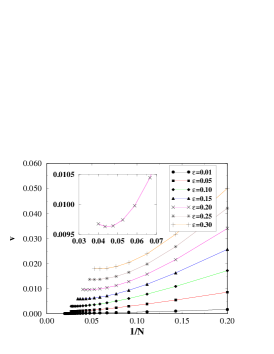
FIG. 9.: Plot of the drift velocity $v$ as function of the inverse chain length $1/N$, for various fixed values of the electric field $\varepsilon$ and $d=1$. Inset: Blow up of $v$ vs. $1/N$ for $\varepsilon=0.2$; a minimum in the velocity can be clearly seen.

In Figure 9 we plotted the velocity as function of the inverse chain length $1/N$ for various values of the electric field. The deviations from the linear regime, where $v\sim\varepsilon/N$, are clearly observable as for sufficiently long chains and not too small fields the drift velocity approaches a non-vanishing value. A closer inspection on the curves reveals that the limiting constant velocity in the asymptotic regime $N\to\infty$ is reached through a minimum in the velocity at a given polymer length $N_{\rm min}$. In our calculations this occurs for any values of the fields in the range $\varepsilon\geq 0.10$. Presumably the minimum is shifted to lengths $N$ much longer than those which can be reached in the present calculation. The existence of a minimum velocity at finite length can be clearly seen in the inset of Fig. 9 which plots $v$ vs. $1/N$ for $\varepsilon=0.2$, but it is present also in other curves. According to our error estimates typical uncertainties in the velocities are at the sixth decimal place, thus error bars are much smaller than all symbol sizes in the figure and inset.

The possible existence of a velocity minimum has given rise to quite some discussions in the past and it is a phenomenon referred to as band inversion (for a review see Ref.[10]). In the band inversion region long polymers migrate faster along the field direction than short ones, a physical situation that looks at first sight somewhat counterintuitive. Band inversion was predicted first in the context of the biased reptation model (BRM) [37], which provides a simplified picture of the physics of polymer reptation in a field, in which fluctuations effects are neglected. More refined analytical calculations in models where fluctuation effects are taken into account still predict the presence of a velocity minimum [38], thus the original result of the BRM was confirmed.

It should be pointed out that the Eq. (15) does not yield any minimum in the velocity as $\partial v/\partial N<0$ for all $N$, thus it cannot be strictly correct. Although our results are limited to the onset of the minimum, we suspect that the minimum is not a very pronounced one so that for longer chains the curves $v$ vs. $1/N$ would appear rather flat. A shallow minimum could have been thus missed in the Monte Carlo simulations of Ref. [16].

Indeed, the data presented in Ref. [16] yield, for instance, $v\approx 0.010$ for $\varepsilon=0.2$ and $N=100$, thus the limiting velocity appears to be approached very slowly from below (see inset of Fig. 9). Other previous simulations by Duke [12] of the RD model yielded instead a quite clear velocity minimum, but it is difficult to judge the quality of his data as no error bars are reported. Probably the inversion effect is somewhat weaker than reported in [12]. We investigated further the effect of $d$ and found that for higher $d$ the minimum appears to be somewhat more pronounced, which may explain the results of Ref. [12], where $d=6$ was taken (the lattice coordination number for an fcc lattice).

Unfortunately, present DMRG computations are limited to the onset of the inversion phenomenon. The problem with the DMRG approach is that it builds up an optimal basis for the stationary state using information of stationary states for shorter chains. Around the band inversion point there is a kind of phase transition from short unoriented polymers to long oriented ones (see for instance Ref. [10]). This change implies that the optimal basis for short chains may be no longer a good one when longer chains are considered. We alleviated somewhat this problem using the DMRG algorithm at fixed $N\varepsilon$, which allows indeed to study slightly longer chains, yet not enough to go deep into the band collapse regime, but sufficient to bring in evidence the velocity minimum.

Originally, it was thought that the drift velocity should be described by a scaling function in terms of the combination $N\varepsilon^{2}$ [39, 40]. It is nowadays believed that the correct scaling form for the velocity should be given by an expression [41, 16]

$$v(\varepsilon,N)=\frac{\varepsilon}{N}\ g(N\varepsilon)$$ (16)

with $g(x)\to g_{0}>0$ for $x\to 0$ and $g(x)\sim x$ for $x\to\infty$ in order to match the known behavior of the velocity at large and small fields. The condition to have band inversion is $\partial v/\partial N=0$ for some $N$ at fixed fields, which is equivalent to the requirement $g(x)=xg^{\prime}(x)$, for a non-zero value of $x=N\varepsilon$. Notice that choosing the most general scaling form $v(\varepsilon,N)=\frac{\varepsilon}{N}\ g(N\varepsilon^{\alpha})$ and from the requirement of $\partial v/\partial N=0$ one still obtains $g(x)=xg^{\prime}(x)$, with $x=N\varepsilon^{\alpha}$.

The scaling behavior of the minimum as function of the field may be used to test the velocity formula. We calculated the polymer length $N_{\rm min}$ at which the minimum of the velocity occurs as function of the applied field $\varepsilon$. If Eq. (16) is correct we expect $\varepsilon\sim 1/N_{\rm min}$. Figure 10 shows a plot of $\ln\varepsilon$ vs. $\ln N_{\rm min}$ for $d=1$. The data show some curvature due to corrections to scaling and approach, for the longest chains analyzed, the asymptote $\varepsilon\sim N^{-\alpha}$, with $\alpha=1.4$, as illustrated in the figure. As $N_{\rm min}$ is increased one observes a systematic decrease of the local slope of the data suggesting that the asymptotic exponent $\alpha<1.4$. In an attempt to reach the asymptotic regime we extrapolated the local slopes of the data in Fig. 10 in the limit $N_{\rm min}\to\infty$, which yield an extrapolated value $\alpha\approx 1.1$, not far from the prediction of Eq.(16), but not fully consistent with it. To prove Eq.(16) more convincingly one would need to investigate longer chains.

FIG. 10.: Plot of $\ln\varepsilon$ vs. $\ln N_{\rm min}$ for $d=1$.

B Correlations and profiles

A more detailed insight in the shapes of the configurations is obtained by plotting averages of the local variables $y_{i}$. The DMRG procedure leads naturally to the determination of the probabilities for two consecutive segments

$$p_{i}(y,y^{\prime})=\langle\,\delta_{y,y_{i}}\,\delta_{y^{\prime},y_{i+1}}\,\rangle.$$ (17)

The probabilities on a single segment follow from these values

$$p_{i}(y)=\sum_{y^{\prime}}p_{i}(y,y^{\prime})=\langle\,\delta_{y,y_{i}}\,\rangle=\sum_{y^{\prime}}p_{i-1}(y^{\prime},y),$$ (18)

which in turn are normalized

$$\sum_{y}p_{i}(y)=1.$$ (19)

The 9 possible values of $p_{i}(y,y^{\prime})$ are restricted by these conditions. One finds another set of relations between these quantities by summing the Master Equation over all but one segment value. Exclusion of an internal segment $y_{i}$ from the summation yields for $y_{i}=y=\pm 1$

$$B^{y}p_{i-1}(0,y)-B^{-y}p_{i-1}(y,0)=$$ (20)

$$B^{y}p_{i}(0,y)-B^{-y}p_{i}(y,0)=v(y).$$ (21)

Note that $v(y)$ is independent of the index $i$ of the segment under consideration. The two relations (20) are an expression of the fact the average velocity of the reptons in the field direction and the curvilinear velocity are constant along the chain. Taking the segment value $y_{j}=0$ one finds

$$v=v(1)-v(-1)=2v(1),$$ (22)

with $v$ the drift velocity. Excluding the end segments from the summation yields the 2 equations ($y=\pm 1$)

$$v(y)=B^{y}p_{1}(y)-dB^{-y}p_{1}(0)$$ (23)

$$v(y)=dB^{y}p_{N}(0)-B^{-y}p_{N}(y)$$ (24)

One observes that the 3 probabilities on the end segments are fixed by the normalization and the 2 equations (23). In general these relations show how delicate the development of the correlations is. In the fieldless case the probability of a configuration factorizes in a product over probabilities of segments. So for $d=1$ the probability on any segment becomes equal to 1/3. Then of course the velocities vanish. Considering the terms linear in the field (or in $B-B^{-1}$) one sees that the drift velocity of the first repton, given by

$$v=Bp_{1}(1)-B^{-1}p_{1}(-1)+d(B-B^{-1})p_{1}(0),$$ (25)

requires a delicate compensation in the linear deviations of the probabilities $p_{1}(y)$ in order to give a value which vanishes as $1/N$ for long chains.

Rather than giving the values of $p_{i}(y)$ we plot the averages

$$\langle\,y_{i}\,\rangle=p_{i}(1)-p_{i}(-1)$$ (26)

and

$$\langle\,y_{i}\,y_{i+1}\,\rangle=p_{i}(1,1)+p_{i}(-1,-1)-p_{i}(1,-1)-p_{i}(1-,1).$$ (27)

FIG. 11.: The profiles for $\varepsilon=0.001$ plotted as function of the reduced distances $l_{N}(i)=(2i-N)/(N-2)$ and $k_{N}(i)=(2i-N+1)/(N-3)$ (with $i=1,2,\ldots N-1$). The number of reptons is fixed at $N=15$.

FIG. 12.: The shapes of the chain for $\varepsilon=0.001$ and various values of $d$. The number of reptons is fixed at $N=15$.

A typical plot for the small $\epsilon$ regime is given in Fig. 11. The global symmetry due to the interchange of head and tail makes the average (26) anti–symmetric with respect to the middle and the average (27) symmetric. One observes that the features increase with the mobility $d$ of the end reptons. The averages give information about the average shape of the chain. In Fig. 12 we translate the averages (26) into average spatial configurations by integrating (summing) the segment values to positions with respect to the middle repton. Clearly the development of the $U$ shape is visible with increasing $d$. The effect is larger at the ends than in the middle.

FIG. 13.: As in Fig. 11 for $d=1$ and varying $\varepsilon$. The number of reptons is fixed at $N=15$.

As an example of the behavior in the intermediate regime (of the velocity profiles Fig. 3) we have plotted in Fig. 13 the situation for $N=15$, $d=1$ and various values of $\epsilon$. For the larger values of $\epsilon$ the average $\langle y_{i}\rangle$ does not change very much but the plateau of the correlations $\langle y_{i}y_{i+1}\rangle$ in the middle keeps rising. We expect that for longer chains a large region in the middle develops where the shape varies weakly with $\epsilon$ and where the correlations between consecutive segments increase. Thus the chain obtains longer stretches which are oriented in the field, either up or down, but which largely compensate, such that the overall shape in the middle remains more or less the same. This is in agreement with the speculations of Barkema et al. [16] on the chain as a stretched sequence of more or less isotropic ”blobs”.

FIG. 14.: The profiles for $d=1$. The number of reptons is fixed at $N=9$.

Finally we show in Fig. 14 the situation for strong $\epsilon$ on a chain of $N=9$ reptons. For the strongest values of $\epsilon$ it is almost exclusively in the $U$ shaped configuration. Note also that the correlations approach 1 except for the middle pair of segments which are on different branches of the $U$. So ultimately the value of the correlation in the middle will approach -1.

Thus we see that the reptating chain develops a rich and delicate pattern of shapes and correlations which are not so easy to catch in simple describing formulae. The difficulty is that there is a different dependence in scale on the parameters $\epsilon$ and $N$ in the middle of the chain and at the ends of the chain. A rough estimate indicates the existence of a zone of length $\sqrt{N}$ at the ends of the chain with the typical bending over of the average $\langle y_{i}\rangle$. In the middle remains a zone of length order $N$, with fairly constant correlations. This splitting up in “bulk” and “surface” behavior which keep each other in balance prevents a systematic expansion in the small parameter $\epsilon$.

VI Discussion

Using the DMRG technique we have determined the properties of the RD model for moderately long chains. At zero and for very small driving fields we could reach chains of the order of $N\approx 100-150$ reptons; for finite fields the lengths are restricted to some 30 reptons. This regime is far outside the domain where exact diagonalization of the reptation matrix is possible. The DMRG results have the advantage, over corresponding Monte Carlo results, of being virtually exact as long as the iteration method converges. Since the DMRG procedure gives simultaneously all the lengths $N$ smaller than the maximum, we can accurately determine the finite size effects on the asymptotic large $N$ behavior.

We find that the renewal time $\tau$ and the diffusion coefficient $D$ are strongly affected by finite size corrections in the regime of these moderately large $N$. Here we have shown that the large finite size corrections, characteristic for the reptation process, manifest themselves as effective exponents for the asymptotic behavior of the renewal time and the diffusion coefficient. We found that DMRG results reveal that, while the leading correction terms, as given by Doi’s theory [26] fit rather well the data for large $N$, they are not sufficient to cause a crossover behavior and higher order corrections need to be included. These finite size effects offer an explanation for the discrepancies between measurement and standard theory. This point can be further tested experimentally by playing with the structure of the end reptons (e.g. branching) and the coordination number of the embedding lattice. We have lumped these aspects in a “dimensionality” parameter $d$, which indeed has surprising effects on the finite size behavior. In particular we expect that chains with short branching ends will be mapped onto small $d$ regimes, where $\tau$ and $D$, according to our results, will scale with effective exponents deviating from the values measured so far. Experimental tests of this prediction will possibly provide new insight for the understanding of the dynamics of entangled polymer melts and concentrated solutions.

We have also established the onset of the so–called band inversion. For fixed driving field and increasing $N$ we observe that the drift velocity goes through a minimum. This is another intriguing effect contained in the RD model. The band inversion has been ascribed to the fact that long polymers in a driving field get oriented and that due to this fixed orientation the drift velocity rather increases with $N$ than decreases as in the non–oriented regime. To see the ultimate asymptotic velocity longer chains than presently possible should investigated.

The DMRG calculations also yield a host of detailed information about the structure of the reptating polymer as for instance the local correlation functions. We have plotted the average values $\langle y_{i}\rangle$ and $\langle y_{i}y_{i+1}\rangle$. We find that the reptating chain develops a rich and delicate pattern of shapes and correlations which are not so easy to catch in simple describing formulae. The difficulty is that there is a different dependence in scale on the parameters $\epsilon$ and $N$ in the middle of the chain and at the ends of the chain. A rough estimate indicates the existence of a zone of length $\sqrt{N}$ at the ends of the chain with the typical bending over of the average $\langle y_{i}\rangle$. In the middle remains a zone of length order $N$, with fairly constant correlations. This splitting up in “bulk” and “surface” behavior which keep each other in balance prevents a systematic expansion in the small parameter $\epsilon$.

We are grateful to G. T. Barkema for helpful discussions and to T. Lodge for drawing our attention to the experimental results of Refs. [8] and [9].

REFERENCES

- [1] P. G. de Gennes, J. Chem. Phys. 55, 572 (1971).
- [2] P. G. de Gennes, Scaling Concepts in Polymer Physics (Cornell University, Ithaca, 1979).
- [3] M. Doi and S. F. Edwards, The Theory of Polymer Dynamics (Oxford University, New York, 1989).
- [4] J. D. Ferry, Viscoelastic Properties of Polymers (Wiley, New York, 1980).
- [5] J. Klein, Nature 271, 143 (1978).
- [6] H. Kim et al., Macromolecules 19, 2737 (1986).
- [7] N. Nemoto et al., Macromolecules 22, 3793 (1989).
- [8] T. P. Lodge, Phys. Rev. Lett.83, 3218 (1999).
- [9] H. Thao, T. P. Lodge, and E. D. von Meerwall, Macromolecules 33, 1747 (2000).
- [10] J.-L. Viovy, Rev. Mod. Phys. 72, 813 (2000).
- [11] M. Rubinstein, Phys. Rev. Lett.59, 1946 (1987).
- [12] T. A. J. Duke, Phys. Rev. Lett.62, 2877 (1989).
- [13] B. Widom, J.-L. Viovy and A. D. Defontaines, J. Phys I France, 1 , 1759 (1991).
- [14] J. M. J. van Leeuwen, J. Phys. I France 1, 1675 (1991).
- [15] M. Prähofer and H. Spohn, Physica A 233, 191 (1996).
- [16] G. T. Barkema, J. F. Marko and B. Widom, Phys. Rev. E49, 5303 (1994).
- [17] M. E. J. Newman and G. T. Barkema, Phys. Rev. E56, 3468 (1997).
- [18] S. R. White, Phys. Rev. Lett.69, 2863 (1992).
- [19] I. Peschel, X. Wang, M. Kaulke and K. Hallberg (Eds.), Density Matrix Renormalization: A New Numerical Method in Physics (Springer, Heidelberg, 1999).
- [20] E. Carlon, A. Drzewiński, and J. M. J. van Leeuwen, Phys. Rev. E64, R010801 (2001).
- [21] T. Nishino, J. Phys. Soc. Jpn. 64, 3598 (1995); E. Carlon and A. Drzewiński, Phys. Rev. Lett.79, 1591 (1997).
- [22] M. Kaulke and I. Peschel, Eur. Phys. J. B 5, 727 (1998); E. Carlon, M. Henkel and U. Schollwöck, Eur. Phys. J. B 12, 99 (1999).
- [23] G. H. Golub and C. F. Van Loan, Matrix Computations (Baltimore, 1996).
- [24] E. Carlon, M. Henkel and U. Schollwöck, Phys. Rev. E63, 036101 (2001).
- [25] J. M. Deutsch and T. L. Madden, J. Chem. Phys. 91, 3252 (1989).
- [26] M. Doi, J. Polym. Sci., Polym. Lett. Ed. 19, 265 (1981); M. Doi, J. Polym. Sci., Polym. Phys Ed. 21, 667 (1983).
- [27] S. T. Milner and T. C. B. McLeish, Phys. Rev. Lett.81, 725 (1998).
- [28] S. T. Milner and T. C. B. McLeish, Macromolecules 30, 2159 (1997).
- [29] M. Fasolo, Tesi di Laurea, Università di Padova, 2001.
- [30] M. Paessens and G. Schütz, preprint cond-mat/0201463.
- [31] K. E. Evans and S. F. Edwards, J. Chem. Soc. Faraday Trans. 2 77, 1891 (1981).
- [32] J. M. J. van Leeuwen and A. Kooiman, Physica A 184, 79 (1992).
- [33] G. T. Barkema and H. M. Krentzlin, J. Chem. Phys. 109, 6486 (1998).
- [34] A. L. Frischknecht and S. T. Milner, Macromolecules 33, 5273 (2000).
- [35] A. B. Kolomeisky, PhD Thesis, Cornell University 1998.
- [36] The expression reported in Eq. (15) fits rather well also the velocity as function of the field for the cage model of electrophoresis. See: A. van Heukelum and H. R. Beljaars, J. Chem. Phys. 113, 3909 (2000).
- [37] J. Noolandi, J. Rousseau, G. W. Slater, C. Turmel, and M. Lalande Phys. Rev. Lett.58, 2428 (1987).
- [38] A. N. Semenov, T. A. J. Duke, and J.-L. Viovy, Phys. Rev. E51, 1520 (1995).
- [39] O. J. Lumpkin, P. Dejardin, and B. H. Zimm, Biopolymers 21, 2315 (1985).
- [40] G. W. Slater and J. Noolandi, Biopolymers 25, 431 (1986).
- [41] T. A. J. Duke, A. N. Semenov, and J.-L. Viovy, Phys. Rev. Lett.69, 3260 (1992).