Exact results on spin glass models

Abstract

Exact and/or rigorous results are reviewed for the Ising and $XY$/Villain spin glasses in finite dimensions, such as the exact energy, correlation identities and a functional relation between the distribution functions of ferromagnetic and spin glass order parameters. This last relation is useful to prove that the phase space is not complex on a line in the phase diagram. The spin wave theory neglecting periodicity is shown to give exact results for the Villain model on a line in the phase diagram. Implications of this fact on the renormalization-group results for the random-phase $XY$/Villain model in two dimensions are discussed.

1 Introduction

The mean-field theory of spin glasses is now well established. The spin glass phase that exists at low temperatures is known to be characterized by a complex phase space and slow dynamics. It is a target of active current investigations to settle whether or not the predictions of the mean-field theory apply to realistic finite-dimensional systems. It is generally difficult to clarify the properties of finite-dimensional systems by analytical methods, and numerical investigations are the main tools of research. The purpose of the present contribution is to overview the available exact/rigorous results on spin glass models in finite dimensions with several new additions to the list. We also prove coincidence of our exact results with the consequences of the spin wave theory for the random-phase $XY$/Villain model. This fact may shed a new light on the significance of existing renormalization group arguments for the two-dimensional random-phase $XY$/Villain model.

2 Ising spin glass

Let us first consider the Ising spin glass described by the Hamiltonian

$$H=-\sum_{\langle ij\rangle}J_{ij}S_{i}S_{j},$$ (1)

where $S_{i}=\pm 1$ and $J_{ij}=\pm J$, namely the $\pm J$ model. The Gaussian model can be treated similarly. This Hamiltonian is invariant under the gauge transformation

$$S_{i}\to S_{i}\sigma_{i},~{}~{}~{}J_{ij}\to J_{ij}\sigma_{i}\sigma_{j},$$ (2)

where $\sigma_{i}$ is another Ising variable fixed arbitrarily at each site. Using this gauge invariance, we can derive many exact or rigorous results [1, 2], some of which are listed below. Unless stated otherwise, the only condition for the following results to hold is that $K=K_{p}$, where $K=\beta J(=J/k_{B}T)$ and $K_{p}$ is a function of $p$ (the probability that the quenched random variable $J_{ij}$ is equal to $J$), $\exp(-2K_{p})=(1-p)/p$. No restrictions exist on the lattice structure or the spatial dimensionality.

The average energy is obtained exactly as

$$[E]=-N_{B}J\tanh K$$ (3)

and the upper bound on the specific heat is

$$k_{B}T^{2}[C]\leq J^{2}N_{B}{\rm sech}^{2}K,$$ (4)

where $N_{B}$ is the number of bonds in the system. The square brackets denote the configurational average. The gauge-invariant correlation function decays exponentially

$$[\langle S_{0}\cdot\tau_{01}\tau_{12}\cdots\tau_{r-1,r}\cdot S_{r}\rangle]=\tanh^{r}K,$$ (5)

where $\tau_{j,j+1}(=\pm 1)$ is the sign of $J_{j,j+1}$, and the pairs of neighbouring sites $(0,1),(1,2),\cdots,(r-1,r)$ connect sites 0 and $r$. The configurational average of the inverse correlation function is identically unity

$$\left[\frac{1}{\langle S_{i}S_{j}S_{k}\cdots\rangle}\right]=1,$$ (6)

and the correlation function satisfies

$$[\langle S_{i}S_{j}\rangle]=[\langle S_{i}S_{j}\rangle^{2}].$$ (7)

By taking the thermodynamic limit in the above correlation identity (7) and then considering the limit of infinite separation of the two sites $i$ and $j$, we conclude that the ferromagnetic order parameter is equal to the spin glass order parameter, $m=q$.

All these results suggest a very special role played by the line defined by $K=K_{p}$ on the phase diagram (Fig. 1), the Nishimori line.

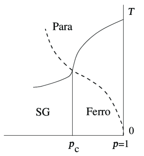
Figure 1: Phase diagram of the $\pm J$ model and the Nishimori line (dashed).

In particular, the relation $m=q$ together with an inequality on the sign of local magnetization [3, 2]

$$M(K,K_{p})=\left[{\rm sgn}\langle S_{i}\rangle\right]\leq M(K_{p},K_{p})$$ (8)

implies that the Nishimori line marks a crossover between the purely ferromagnetic region (where $m>q$ and $M$ is a decreasing function of $T$) and a randomness-dominated region (where $m<q$ and $M$ is an increasing function of $T$) within the ferromagnetic phase.

An important generalization of the relation $m=q$ is the functional identity $P_{m}(x)=P_{q}(x)$ under the same condition $K=K_{p}$ [4, 2]. Here, $P_{m}(x)$ is the distribution function of magnetization

$$P_{m}(x)=\left[\frac{\sum_{S}\delta\left(x-\frac{1}{N}\sum_{i}S_{i}\right)e^{-\beta H}}{\sum_{S}e^{-\beta H}}\right]$$ (9)

and $P_{q}(x)$ is the distribution of spin glass order parameter defined in terms of two real replicas

$$P_{q}(x)=\left[\frac{\sum_{S}\sum_{\sigma}\delta\left(x-\frac{1}{N}\sum_{i}S_{i}\sigma_{i}\right)e^{-\beta H(S)-\beta H(\sigma)}}{\sum_{S}\sum_{\sigma}e^{-\beta H(S)-\beta H(\sigma)}}\right].$$ (10)

The proof of the identity $P_{m}(x)=P_{q}(x)$ is relatively straightforward if we apply the gauge transformation to the expression (9) and use the condition.

Since the distribution function of magnetization $P_{m}(x)$ is always composed of at most two simple delta functions located at $\pm m$, the identity $P_{m}(x)=P_{q}(x)$ implies that the distribution of the spin glass order parameter $P_{q}(x)$ also has the same simple structure. This excludes the possibility that a complex structure of the phase space, which should be reflected to a non-trivial functional form of $P_{q}(x)$, exists on the Nishimori line $K=K_{p}$. Thus a spin glass (or mixed ferromagnetic) phase of the mean-field type, if it exists in finite dimensions, should lie away from the line in the phase diagram.

3 Random-phase $XY$ and Villain models

The same type of argument applies to the random-phase $XY$ model (gauge glass)

$$H=-J\sum_{\langle ij\rangle}\cos(\theta_{i}-\theta_{j}-A_{ij})$$ (11)

with the phase distribution

$$P(A_{ij})\propto e^{K_{p}\cos A_{ij}},$$ (12)

and the random-phase Villain (or periodic Gaussian) model with nearest-neighbour Boltzmann factor

$$e^{V(\theta_{i}-\theta_{j}-A_{ij})}=\sum_{m=-\infty}^{\infty}e^{-K(\theta_{i}-\theta_{j}-A_{ij}-2\pi m)^{2}/2},$$ (13)

where the phase variable obeys

$$P(A_{ij})\propto\sum_{m=-\infty}^{\infty}e^{-K_{p}(A_{ij}-2\pi m)^{2}/2}.$$ (14)

We note here that the periodic distribution (14) is equivalent to a non-periodic Gaussian distribution (often used in the literature) because (13) is periodic in $A_{ij}$. The Villain model (13) is often used as a low-temperature effective model of the $XY$ model (11), in particular in the analysis of the Kosterlitz-Thouless transition in two dimensions. We shall see that the results for the Villain model indeed agree with those for the $XY$ model at sufficiently low temperatures.

These models are invariant under the gauge transformation

$$\theta_{i}\to\theta_{i}+\phi_{i},~{}~{}~{}A_{ij}\to A_{ij}+\phi_{i}-\phi_{j}.$$ (15)

We simply list the results for the random-phase $XY$ model that have been obtained using gauge invariance [1, 5, 2], corresponding to (3), (4), (5), (6) and (7) for the Ising case,

$$[E]=-N_{B}J\,\frac{I_{1}(K)}{I_{0}(K)}$$ (16)

$$k_{B}T^{2}[C]\leq J^{2}N_{B}\left(\frac{1}{2}+\frac{I_{2}(K)}{2I_{0}(K)}-\left(\frac{I_{1}(K)}{I_{0}(K)}\right)^{2}\right)$$ (17)

$$\left[\langle e^{i(\theta_{0}-A_{01}-A_{12}-\cdots-A_{r,r-1}-\theta_{r})}\rangle\right]=\left(\frac{I_{1}(K)}{I_{0}(K)}\right)^{r}$$ (18)

$$\left[\frac{1}{\langle e^{i\sum_{j}a_{j}\theta_{j}}\rangle}\right]=1$$ (19)

$$\left[\langle e^{i(\theta_{0}-\theta_{r})}\rangle\right]=\left[\left|\langle e^{i(\theta_{0}-\theta_{r})}\rangle\right|^{2}\right],$$ (20)

where $I_{j}(K)$ is the modified Bessel function and the $a_{j}$ are arbitrary numbers. All these equations hold on any lattice in any dimension as long as the condition $K=K_{p}$ is satisfied.

Correlation functions of bond variables can also be evaluated under the condition $K=K_{p}$:

$$\left[\langle\cos(\theta_{0}-\theta_{1}-A_{01})\cos(\theta_{r}-\theta_{r+1}-A_{r,r+1})\rangle\right]=\left(\frac{I_{1}(K)}{I_{0}(K)}\right)^{2}$$ (21)

$$\left[\langle\sin(\theta_{0}-\theta_{1}-A_{01})\sin(\theta_{r}-\theta_{r+1}-A_{r,r+1})\rangle\right]=0,$$ (22)

where $(01)$ and $(r,r+1)$ are pairs of neighbouring sites. The second identity for the sine correlation is particularly interesting since it means the absence of spatial correlation between chirality degrees of freedom [2].

An identity between the distribution functions of ferromagnetic and spin glass order parameters can also be proved, $P_{m}(z)=P_{q}(z)$ for $K=K_{p}$, where the distribution function of the ferromagnetic order parameter is defined as

$$P_{m}(z)=\left[\left\langle\delta\left(z-\frac{1}{N}\sum_{j}e^{i\theta_{j}}\right)\right\rangle\right]$$ (23)

and that of the spin glass order parameter is given using two replicas as in (10)

$$P_{q}(z)=\left[\left\langle\delta\left(z-\frac{1}{N}\sum_{j}e^{i(\theta_{j}-\phi_{j})}\right)\right\rangle\right],$$ (24)

where two replicas of the same system have dynamical variables $\{\theta_{j}\}$ and $\{\phi_{j}\}$.

The random-phase Villain model can be treated in the same manner. The results corresponding to (16), (18), (19) and (20) are, under the condition $K=K_{p}$ and with the notation $T=K^{-1}$,

$$\left[\langle e^{i(\theta_{0}-\theta_{1}-A_{01})}\rangle\right]=e^{-T/2}$$ (25)

$$\left[\langle e^{i(\theta_{0}-A_{01}-A_{12}-\cdots-A_{r,r-1}-\theta_{r})}\rangle\right]=e^{-rT/2}$$ (26)

$$\left[\frac{1}{\langle e^{i\sum_{j}a_{j}\theta_{j}}\rangle}\right]=1$$ (27)

$$\left[\langle e^{i(\theta_{0}-\theta_{r})}\rangle\right]=\left[\left|\langle e^{i(\theta_{0}-\theta_{r})}\rangle\right|^{2}\right].$$ (28)

Correlations between bond variables satisfy, similarly to (21) and (22),

$$\left[\langle\cos(\theta_{0}-\theta_{1}-A_{01})\cos(\theta_{r}-\theta_{r+1}-A_{r,r+1})\rangle\right]=e^{-T}$$ (29)

$$\left[\langle\sin(\theta_{0}-\theta_{1}-A_{01})\sin(\theta_{r}-\theta_{r+1}-A_{r,r+1})\rangle\right]=0.$$ (30)

It can also be proved that the functional identity $P_{m}(z)=P_{q}(z)$ holds if $K=K_{p}$. These relations for the Villain model agree with the corresponding results for the $XY$ model in the low-temperature limit.

It is clear that the Nishimori line $K=K_{p}$ plays key roles in the determination of the system properties also in the present continuous-variable system. This line is expected to mark the crossover between the pure ferromagnetic-like region and a randomness-dominated region within the ferromagnetic phase.

4 Spin wave theory

The random-phase $XY$ model has often been analyzed by the spin wave theory, particularly in two dimensions. In the spin wave theory one expands the cosine interaction (11) to second order of the argument, assuming that the argument is small at low temperatures

$$\cos(\theta_{i}-\theta_{j}-A_{ij})\approx 1-\frac{1}{2}(\theta_{i}-\theta_{j}-A_{ij})^{2}.$$ (31)

It will be assumed that the quenched gauge variable $A_{ij}$ is also Gaussian-distributed with variance $\sigma\equiv K_{p}^{-1}$.

An important difference between the spin wave theory (31) and the Villain model (13) is in periodicity. The latter model is periodic in the variables $\theta_{i},\theta_{j}$ and $A_{ij}$ with period $2\pi$ as in the original $XY$ model (11) whereas the spin wave theory (31) neglects periodicity. Periodicity of the Hamiltonian (11) or the Boltzmann factor (13) is directly related with the existence of vortices, which leads to the Kosterlitz-Thouless transition in two dimensions [6]. It is then expected that the spin wave theory fails to reproduce important characteristics of the $XY$/Villain model. Surprisingly this is not the case at least for the relations we have derived above using gauge transformation as shown below.

The spin-wave Hamiltonian is Gaussian, and everything can be evaluated explicitly in any dimension. The results corresponding to (25) to (30) are given below. Note that the following relations are valid for any $T$ and $\sigma$ in contrast to the results of the gauge theory which require $T=\sigma~{}(K=K_{p})$. The spatial dimension is arbitrary.

$$\left[\langle e^{i(\theta_{0}-\theta_{1}-A_{01})}\rangle\right]=\exp\left\{(T-\sigma)G_{01}-\frac{\sigma}{2}\right\}$$ (32)

$$\left[\langle e^{i(\theta_{0}-A_{01}-A_{12}-\cdots-A_{r,r-1}-\theta_{r})}\rangle\right]=\exp\left\{(T-\sigma)G_{0r}-\frac{r\sigma}{2}\right\}$$ (33)

$$\left[\frac{1}{\langle e^{i\sum_{j}a_{j}\theta_{j}}\rangle}\right]=\exp\left\{\frac{T}{2}\sum_{i,j}a_{i}a_{j}G_{ij}-\frac{\sigma}{2}\sum_{i,j}a_{i}a_{j}G_{ij}\right\}$$ (34)

$$\left[\langle e^{i(\theta_{0}-\theta_{r})}\rangle\right]=e^{(T+\sigma)G_{0r}}$$ (35)

$$\left[\left|\langle e^{i(\theta_{0}-\theta_{r})}\rangle\right|^{2}\right]=e^{2TG_{0r}}.$$ (36)

Here $G_{0r}$ is the lattice Green function. Its explicit form is, for example for the two-dimensional square lattice,

$$G_{0r}=\frac{1}{N}\sum_{k}\frac{\cos\mbox{\boldmath$k$}\cdot\mbox{\boldmath$r$}-1}{4-2\cos k_{1}-\cos k_{2}}.$$ (37)

Correlations of bond variables can also be evaluated by the spin wave theory:

$$\left[\langle\cos(\theta_{0}-\theta_{1}-A_{01})\cos(\theta_{r}-\theta_{r+1}-A_{r,r+1})\rangle\right]=\frac{1}{2}C_{r-}+\frac{1}{2}C_{r+}$$ (38)

$$\left[\langle\sin(\theta_{0}-\theta_{1}-A_{01})\sin(\theta_{r}-\theta_{r+1}-A_{r,r+1})\rangle\right]=\frac{1}{2}C_{r-}-\frac{1}{2}C_{r+},$$ (39)

where $C_{r\pm}$ is, in the case of the square lattice,

$$C_{r\pm}=\exp\left\{\frac{\sigma-T}{N}\sum_{k}\frac{(1-\cos k_{1})(1\pm\cos\mbox{\boldmath$k$}\cdot\mbox{\boldmath$r$})}{2-\cos k_{1}-\cos k_{2}}-\sigma\right\}.$$ (40)

All these relations (32) to (39) reduce to the corresponding Villain results (25) to (30) if $T=\sigma$. This is a surprising conclusion because it means that, if $T=\sigma$, periodicity of the Villain model (or vortex degrees of freedom) has no effects at all on the quantities calculated above. The spin wave theory gives the exact solution and rigorous relations for the Villain model.

5 Conclusion

We have shown a number of exact/rigorous results for the Ising spin glass and random-phase $XY$ and Villain models. These models can be treated by the gauge theory, a method exploiting gauge invariance of the Hamiltonian or the Boltzmann factor. The exact solution for the energy and rigorous relations for the specific heat and correlation functions have been derived under the condition of $K=K_{p}$. The results for the $XY$ model have been shown to reduce to those for the Villain model in the low-temperature limit.

We have used the spin wave theory to calculate various correlation functions for the random-phase $XY$/Villain models. It has been found that the spin wave theory, which neglects periodicity of the system, gives the exact expressions for the quantities that have been treated by the gauge theory for the Villain model as long as the condition $K=K_{p}$ is satisfied. Thus the effects of periodicity, or the vortex degrees of freedom, completely disappear at least from these quantities if $K=K_{p}$.

It is of course expected that periodicity plays essential roles in the determination of the explicit exact form of the correlation function $[\langle e^{i(\theta_{0}-\theta_{r})}\rangle]$ of the Villain model since, otherwise, the spin wave theory would be valid for an arbitrarily high temperature, implying that the low-temperature Kosterlitz-Thouless (in two dimensions) or the ferromagnetic (in higher dimensions) phase would extend to the infinite-temperature limit. Nevertheless, the present conclusion of the exact relations for the energy and other quantities by the spin wave theory is never trivial, in consideration of the fact that the Nishimori line $K=K_{p}~{}(T=\sigma)$ seems to occupy no special status in the phase diagram according to the renormalization-group treatment of the two-dimensional Villain model [7, 8, 9]. The renormalization group, rather, predicts that the line defined by $T=2\sigma$ separates the usual ferromagnetic region and the vortex-freezing region within the ferromagnetic phase. One possibility is that current renormalization group treatments miss some important aspects of the system, thus identifying the line $T=2\sigma$ as the crossover line instead of the line $T=\sigma$. Further investigations are necessary to clarify this point.

References

- [1] H. Nishimori, Prog. Theor. Phys. 66, 1169 (1981).
- [2] H. Nishimori, Statistical Physics of Spin Glasses and Information Processing : An Introduction, Oxford Univ. Press (Oxford, 2001).
- [3] H. Nishimori, J. Phys. Soc. Jpn. 62, 2973 (1993).
- [4] H. Nishimori and D. Sherrington, In Disordered and Complex Systems, Eds. P. Sollich, A. C. C. Coolen, L. P. Hughston and R. F. Streater, AIP Conference Proceedings 553 (AIP, Melville, New York, 2001).
- [5] Y. Ozeki and H. Nishimori, J. Phys. A 26, 3399 (1993).
- [6] J. M. Kosterlitz and D. J. Thouless, J. Phys. C 6, 1181 (1973).
- [7] S. Scheidl, Phys. Rev. B 55, 457 (1997).
- [8] L.-H. Tang, Phys. Rev. B 54, 3350 (1997).
- [9] D. Carpentier and P. Le Doussal, Nucl. Phys. B 588 [FS], 565 (2000).