Classical electrons in laterally coupled diatomic 2D artificial molecule

Abstract

Structural properties of a finite number ($N=2-20$) of point charges (classical electrons) confined laterally in a two-dimensional two-minima potential are calculated as a function of the distance ($d$) between the minima. The particles are confined by identical parabolic potentials and repel each other through a Coulomb potential. Both ground state and metastable electron configurations are discussed. At zero distance previous results of other calculations and experiments are reproduced. Discontinuous transitions from one configuration to another as a function of $d$ are observed for $N=6,8,11,16,17,18,19$.

I INTRODUCTION

Quantum dots (sometimes called artificial atoms) are nanoscale semiconductor structures where a small number of electrons are confined into a small spatial region.Ashoori (1996); Kastner (1993) The electron motion is usually further restricted to two dimensions. There is strong theoretical evidence for the existence of a limit where the electron system crystallises to Wigner molecules, which is seen as the localisation of the electron density around positions that minimise the Coulomb repulsion. Egger et al. (1999); Reimann et al. (2000); Creffield et al. (1999); Reusch et al. (2001); Harju et al. ; Koskinen et al. (1997); Maksym et al. (2000) In the limit of weak confinement (low density) or a very strong magnetic field the quantum effects are quenched or obscured and the classical electron correlations start to dominate the properties of the system. The ultimate limit is a purely classical system where only the Coulomb repulsion between the electrons defines the ground state. The problem reduces to finding the classical positions of electrons (which depend on the forms of the confining and the interaction potentials) that minimise the total energy of the system.

There is growing interest in calculatingImamura et al. (1999); Nagaraja et al. (1999); Partoens and Peeters (2000); Chakraborty et al. (1991); Wensauer et al. (2000); Kolehmainen et al. (2000); Jannouleas and Landman (2001) and measuringLivermore et al. (1996); Oosterkamp et al. (1998); Brodsky et al. (2000) the properties of coupled quantum dots. Due to the 2D nature of quantum dots the two-atom system is different whether the quantum dots are coupled in the plane in which the electrons are confined (laterally coupled) or in the perpendicular direction (vertically coupled). Especially for laterally coupled quantum dots only a limited number of studies have appeared.Chakraborty et al. (1991); Wensauer et al. (2000); Kolehmainen et al. (2000); Jannouleas and Landman (2001) Classical studies serve as a good starting point for more demanding quantum mechanical calculations. Moreover, the study of classical electrons in vertically coupled artificial atoms has revealed interesting structural transitions in the ground state electron configurations as a function of the distance between the atoms.Partoens et al. (1997)

Apart from quantum dots in the classical limit the point charges in 2D can be used to model also other physical systems. Examples include vortex lines in superconductors and superfluids and electrons on the surface of liquid He (see Ref. Kong et al., 2001 and references therein). In the theoretical field, the ground state configurations of a confined classical 2D electron system have been studied in the case of a single artificial atom in Refs. Kong et al., 2001; Bolton and Rössler, 1993; Bedanov and Peeters, 1994; Lai and I, 1999; Date et al., 1998; Campbell and Ziff, 1979; Schweigert and Peeters, 1995 and for the vertically coupled artificial atom molecule as a function of the inter-atom distance in Ref. Partoens et al., 1997. Recently, also some experimental studies of 2D confined charged classical particle systems have appeared to reflect the classical cluster patterns in 2D.Juan et al. (1998); Saint Jean et al. (2001)

Classical point charges in a two-dimensional infinite plane crystallise into a hexagonal lattice at low temperatures. Parabolic confinement in the artificial atom, on the other hand, favours circularly symmetric solutions. The ground state configuration is thus determined by two competing effects, circular symmetry and hexagonal coordination, thus resulting in non-trivial particle configurations. The reported configurations of the electron clusters in a single artificial atom do not all agree between different studies. The differences can be partly explained by the different forms of confinement and interaction potentials. However, when the number of particles, $N$, confined in the atom is one of the following $N=2-5,7,10,12,14,19$ all results are in agreement while differences appear for $N=6,8,9,11,13,15-18,20$ (for $N\leq 20$).

In this paper we consider two laterally coupled artificial atoms and classical electrons in the molecule. The changes in the ground state electron configurations are studied for $N=2-20$ electrons in the molecule as the inter-atom distance is changed. The energies of the metastable states are also calculated at different distances and their role in the structural transitions in the ground state electron configurations is discussed. We also reproduce electron configurations of the single parabolic artificial atom. The differences between different calculations and experimental results are discussed in the limit of single atom.

II Monte Carlo simulation

The classical electrons in the artificial atom molecule are modelled with the Hamiltonian

$$H = \frac{1}{2}\ m^{*}\omega_{0}^{2}\ \sum_{i=1}^{N}\min\left[({\vec{r}_{i}}-d/2)^{2},({\vec{r}_{i}}+d/2)^{2}\right]$$ (1)

$$+ \frac{e^{2}}{4\pi\epsilon_{0}\epsilon}\ \sum_{i<j}\frac{1}{|{\vec{r}_{i}}-{\vec{r}_{j}}|}.$$

Each of the $N$ electrons is described with coordinates $\vec{r_{i}}=(x_{i},y_{i})$ in two-dimensional space. The harmonic confinements are positioned symmetrically around the origin with distance $d$ between the minima. $m^{*}$ is the electron effective mass, $\omega_{0}$ the confinement strength and $\epsilon$ the dielectric constant. We measure the energy in meV and distance in Å. The confinement strength was set to $\hbar\omega_{0}=3$ meV and typical GaAs parameters were chosen to the effective mass and the dielectric constant: $m^{*}=0.067\ m_{e}$ and $\epsilon=13$. The calculated energy values and distances could be scaled to correspond to different values of $\omega_{0},\ m^{*},\ \epsilon$, but changing the parameters also changes the effective distance between the minima, $d$, and then the minimum energy configuration may not be the same anymore. Therefore we have have one significant parameter in the system, $d$, which scales as $\propto(m^{*}\omega_{0}^{2}\epsilon)^{-1/3}$.

The minimum energy as a function of the positions of the particles, $E_{tot}=\min\ E({\vec{r}_{1}},...,{\vec{r}_{N}})$, is solved with a standard Metropolis Monte Carlo method Metropolis et al. (1953) starting from a randomly chosen initial electron configuration ${\vec{r}_{1}},...,{\vec{r}_{N}}$. The accuracy and simulation time needed with the Metropolis algorithm was found to be well sufficient for the current problem. We compared the calculated energies in the limit of a single artificial atom to those given in Ref. Kong et al., 2001, and the results were found to be in complete agreement within the given accuracy.

In the simulations we choose four different distances between the atoms and perform 300 test runs at each particle number ($N=2-20$) and distance ($d=0,200,600$ and $1000$ Å). In addition to minimum energy configurations we also obtain metastable states that are higher in energy compared to the ground state.

When the ground and metastable states are obtained at $d=0,200,600,1000$ Å  we study the structural transitions between ground state electron configurations at the intermediate distances. The electron configurations obtained from the fixed $d$ calculations are taken as an input to Monte Carlo minimisations where the attempt step is set so small that the electron configuration cannot change to another. Then the distance is slightly altered ($d\rightarrow d\pm 1$ Å) and a new energy with slightly modified positions is calculated for the configuration defined by the input. The calculated new configuration is taken as an input to the next calculation with a new distance between the atoms, and so all distances between $d=0,200,600,1000$ Å are well sampled. However, it may happen that a configuration becomes unstable as the distance is changed. In that case the simulation converges to some other stable configuration, which can be seen as a sudden jump to a new energy value in the $E(d)$-plots. The energies of all states are studied as a function of the distance and structural transitions in the ground state configurations are examined.

III Results

The results for the ground and metastable states are summarised in Table 1. The electron configurations are given at four different distances between the artificial atoms. The ground state energy and the corresponding configuration at the four distances is represented in the row following the particle number $N$. If there exist metastable states at the given $N$ and $d$ the energy difference $\Delta E/N$ to the ground state and the electron configuration for the metastable state is also reported. However, not all metastable configurations are marked in Table 1, since when starting the simulation from random positions more electrons can be trapped in one artificial atom than in the other. Only metastable states with either the same number of electrons per atom (for even $N$) or only one more at one than the other atom (for odd $N$) are reported. The notation for the configurations in a single artificial atom is chosen so that electrons are thought to be organised in (nearly) concentric shells around the potential minimum: (N₁,N₂,N₃), where N₁ denotes the number of electrons in the innermost shell, N₂ the next shell and N₃ the number of electrons in the outermost shell. (For $N\leq 20$ only three shells are occupied). For laterally coupled two-atom artificial molecule we have chosen the following notation for configurations: At $d=200$ Å the configuration is marked as if it would still be on a single atom centred around the midpoint connecting the two atoms. At $d=600$ and $1000$ Å the configurations are given as configurations of two separated atoms.

For example, as Table 1 and Fig 1 (a) indicate, with eight particles in the single artificial atom ($d=0$ Å) the ground state is (1,7), one electron in the centre and seven electrons in the circular shell, and there exist no metastable states. At $d=200$ Å a new ground state has appeared with configuration (2,6) (Fig. 1 (b)) while (1,7) has changed to a metastable state (see also Table 1). At distances $d=600$ Å  and $d=1000$ Å the notation is changed to two-atom configurations and for $N=8$ the ground state is marked with (4),(4), see Figs. 1 (c) and (e).

The notation for configurations is not always exhaustive. The relative orientation of different shells and the relative orientations of the configurations of the two atoms at $d=600,1000$ Å do not always become clear from Table 1. For example, when either or both atoms are left with four electrons ($N=7,8,9$), the orientation of the square(s) relative to the other atom changes as the distance is increased. At smaller distances the position of the square of four electrons is such that the tips of the squares are in the same line with the positions of the minima (see Fig. 1 (c) for $N=8$ at $d=600$ Å). As the distance is increased the square (or two squares with $N=8$) turns onto its side (see Fig. 1 (e) for $N=8$ at $d=1000$ Å). For $N=8$ at $d=600$ Å there also exists a metastable state where one of the squares is lying on its side and the other on the tip (Fig. 1 (d)). Even though we divide electrons into shells in our notation it does not mean that the shells are strictly circular even for $d=0$. This can be seen clearly for $N=12$ in Fig 1 (f), where the outer shell resembles more like an incomplete triangle with the tips missing. The configuration marked with (1,5)^∗ in the two-atom configurations in Table 1 cannot be identified strictly to (6) but neither to (1,5). Therefore we choose the notation (1,5)^∗ to describe the configuration. The difference between (1,5)^∗ and (1,5) can be seen with the (1,5)^∗,(1,5) metastable state in Fig. 1 (g). The configurations of the ground and metastable states for $N=13$ at $d=200$ Å are marked in the same way in the Table, but are different as can be seen in Figs. 1 (h) and (i). For the highest energy metastable state for $N=17,d=200$ Å the two-atom notation would have described the configuration better, Fig. 1 (l). One metastable state for $N=19$ and the ground state and one metastable state for $N=20$ at $d=200$ Å could not be described with the shell structure notation. The configurations are depicted in Figs. 1 (m),(n) and (o), respectively.

$\begin{array}[]{|c|c|c|}\hline\cr\includegraphics*[height=71.13188pt]{Fig_1a.ps}&\includegraphics*[height=71.13188pt]{Fig_1b.ps}&\includegraphics*[height=71.13188pt]{Fig_1c.ps}\\ \hline\cr\includegraphics*[height=71.13188pt]{Fig_1d.ps}&\includegraphics*[height=71.13188pt]{Fig_1e.ps}&\includegraphics*[height=71.13188pt]{Fig_1f.ps}\\ \hline\cr\includegraphics*[height=71.13188pt]{Fig_1g.ps}&\includegraphics*[height=71.13188pt]{Fig_1h.ps}&\includegraphics*[height=71.13188pt]{Fig_1i.ps}\\ \hline\cr\includegraphics*[height=71.13188pt]{Fig_1j.ps}&\includegraphics*[height=71.13188pt]{Fig_1k.ps}&\includegraphics*[height=71.13188pt]{Fig_1l.ps}\\ \hline\cr\includegraphics*[height=71.13188pt]{Fig_1m.ps}&\includegraphics*[height=71.13188pt]{Fig_1n.ps}&\includegraphics*[height=71.13188pt]{Fig_1o.ps}\\ \hline\cr\end{array}$

Figure 1: (a) - (o). Electron configurations of selected ground and metastable states. The energy per particle ($E/N$) of a ground state configuration and the energy difference to the ground state per particle ($\Delta E/N$) for metastable configuration is given. The configuration is marked on the lower right corner. To make it easier to distinguish different configurations and the distance between the minima ($d=0,200,600,1000$ Å) a circle with 330 Å radius is plotted around each parabolic potential minimum. A dashed circle indicates a metastable state.

Table 1: Ground and metastable configurations and corresponding energies in meV/particle at four studied distances ($d=0,200,600,1000$ Å). The energies of metastable states, $\Delta E/N$, are given as meV/particle above the ground state energy. The configurations of electron clusters in the two-atom molecule are described with concentric shells located around the centre of the system at $d=0,200$ Å and as two separate electron clusters located near the minimum of one of the two atoms at $d=600,1000$ Å.

	$d=0$ Å			$d=200$ Å			$d=600$ Å			$d=1000$ Å
N	$E/N$	$\Delta E/N$	config.	$E/N$	$\Delta E/N$	config.	$E/N$	$\Delta E/N$	config.	$E/N$	$\Delta E/N$	config.
	[meV]	[meV]		[meV]	[meV]		[meV]	[meV]		[meV]	[meV]
2	2.736		(2)	1.777		(2)	0.875		(1),(1)	0.546		(1),(1)
3	4.780		(3)	3.894		(3)	2.940		(1),(2)	2.541		(1),(2)
4	6.696		(4)	5.588		(4)	4.351		(2),(2)	3.795		(2),(2)
5	8.531		(5)	7.340		(5)	5.915		(2),(3)	5.244		(2),(3)
		+0.099	(1,4)
6	10.231		(1,5)	8.939		(6)	7.234		(3),(3)	6.395		(3),(3)
		+0.074	(6)		+0.033	(1,5)
7	11.816		(1,6)	10.459		(1,6)	8.664		(3),(4)	7.720		(3),(4)
8	13.384		(1,7)	11.933		(2,6)	9.932		(4),(4)	8.850		(4),(4)
					+0.016	(1,7)		+0.003	(4),(4)
9	14.913		(2,7)	13.335		(2,7)	11.246		(4),(5)	10.097		(4),(5)
		+0.022	(1,8)
10	16.361		(2,8)	14.680		(2,8)	12.441		(5),(5)	11.195		(5),(5)
		+0.012	(3,7)
11	17.746		(3,8)	16.053		(3,8)	13.701		(5),(1,5)∗	12.361		(5),(1,5)
					+0.003	(2,9)
12	19.111		(3,9)	17.354		(3,9)	14.873		(1,5)∗,(1,5)∗	13.434		(1,5),(1,5)
		+0.011	(4,8)		+0.004	(4,8)		+0.011	(1,5)∗,(1,5)
13	20.433		(4,9)	18.624		(4,9)	16.048		(1,5)∗,(1,6)	14.511		(1,5),(1,6)
					+0.024	(4,9)
14	21.738		(4,10)	19.854		(4,10)	17.168		(1,6),(1,6)	15.518		(1,6),(1,6)
		+0.014	(5,9)
15	23.010		(5,10)	21.072		(5,10)	18.302		(1,6),(1,7)	16.587		(1,6),(1,7)
		+0.029	(1,5,9)		+0.035	(5,10)					+0.234	(1,6),(2,6)
16	24.259		(1,5,10)	22.271		(6,10)	19.373		(1,7),(1,7)	17.583		(1,7),(1,7)
		+0.009	(5,11)		+0.006	(5,11)					+0.024	(1,7),(2,6)
17	25.473		(1,6,10)	23.448		(6,11)	20.468		(1,7),(2,7)	18.611		(1,7),(2,7)
		+0.005	(1,5,11)		+0.010	(1,6,10)		+0.006	(1,7),(1,8)		+0.018	(1,7),(1,8)
					+0.016	(1,5,11)					+0.023	(2,6),(2,7)
					+0.018	(6,11)					+0.041	(2,6),(1,8)
18	26.660		(1,6,11)	24.597		(1,6,11)	21.522		(1,8),(2,7)	19.579		(2,7),(2,7)
		+0.026	(1,7,10)		+0.006	(6,12)		+0.001	(1,8),(2,7)		+0.017	(2,7),(1,8)
19	27.841		(1,6,12)	25.728		(1,6,12)	22.572		(2,7),(2,8)	20.569		(2,7),(2,8)
		+0.003	(1,7,11)		+0.004	(1,7,11)		+0.001	(1,8),(2,8)		+0.016	(1,8),(2,8)
					+0.016	-
20	29.000		(1,7,12)	26.843		-	23.583		(2,8),(2,8)	21.585		(2,8),(2,8)
		+0.024	(1,6,13)		+0.001	-
					+0.003	(2,7,11)

As the distance between the atoms is increased it is not always clear whether the electrons just follow the two atoms drawn apart and continuously change to two separated atoms. Sometimes metastable states change to a ground state and the ground state to a metastable state as the distance between the atoms is increased. The clearest example can be seen in Table 1 for six electrons between $d=0$ and $d=200$ Å. At $d=0$ the (1,5) configuration is the ground state and (6) the metastable state. At $d=200$ Å it is the other way around: (6) is the ground and (1,5) a metastable state. The energy as a function of distance for two alternative configurations is shown in Fig.2 (a). The transition point, marked with a small circle, is at $d=111.6$ Å. The transition is continuous with respect to energy as a function of distance, but the curvature of the $E(d)$-curve is different and therefore the first derivative of energy with respect to $d$ is discontinuous. This is a first-order discontinuous structural transition in the electron configuration. Hereafter, by discontinuous structural transitions we mean the qualitative change in the ground state electron configuration which is discontinuous with respect to $\partial E/\partial d$ at the transition point.

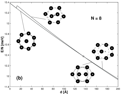
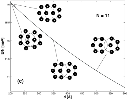
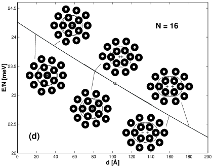
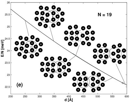
Figure 2: (a) - (e). Energy per particle as a function of distance for $N=6,8,11,16,19$. The small circle indicates the transition point. To make it easier to distinguish different configurations and the distance between the minima a circle with 330 Å radius is plotted around each parabolic minimum. A dashed circle indicates a metastable state.

In addition to $N=6$, for $N=8,11,16$ and $19$ one qualitative change in the electron configuration is observed as a function of $d$. For $N=8$ at $d=135.9$ Å the electron configuration changes from (1,7) to (2,6), see Fig 2 (b). Notice that the (2,6) configuration is not stable at the limit of one atom and becomes unstable approximately below $d=17$ Å. For $N=11$ there exists one metastable state, (2,9), at $d=200$ Å, which at $214.2$ Å changes to a ground state as is depicted in Fig. 2 (c). With $N=16$ the configuration changes from (1,5,10) to (6,10) at $d=102.4$ Å. The energy differences between ground and metastable states are small and metastable states exist only in the proximity of the transition point (Fig. 2 (d)). At $d=80$ Å  the (1,5,10) configuration which is plotted below the energy curve is still the ground state and the (6,10) configuration plotted above the energy curve has appeared as a metastable state. For $N=19$ Fig. 2 (e) shows how the (1,6,12) configuration, which is the ground state at $d=200$ Å, has changed to a rather unsymmetric configuration at $d=250$ Å. This unsymmetric configuration changes continuously to (2,8),(1,8) (lower middle plot in (e)) which at $586.0$ Å  changes discontinuously to (2,8),(2,7) configuration. The (2,8),(2,7) configuration appears approximately at $415$ Å as a metastable state. The (1,8),(2,8) persists as a metastable state to the greatest studied distance of $1000$ Å as is also indicated in Table 1. The other metastable states at $d=0$ and $200$ Å do not change to a ground state.

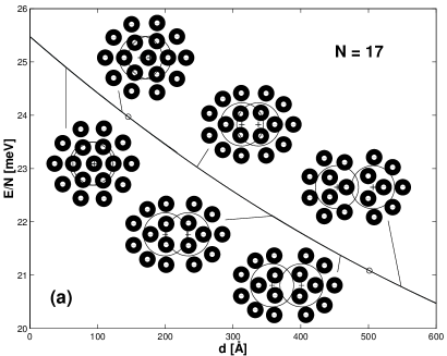
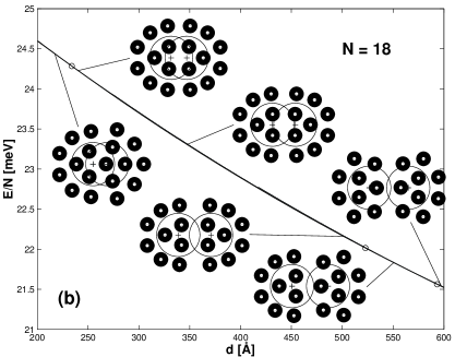
Figure 3: Energy as a function of distance for $N=17$ and $N=18$ with the ground state configurations along the energy curve. The small circles indicate the discontinuous structural transition points.

More than one discontinuous transformation in the electron configurations is found for $N=17$ and $18$, see Figs. 3 (a) and (b). For $N=17$ the (1,6,10) changes to (6,11) at $d=145.0$ Å. The (6,11) configuration parts to (1,7),(1,8) two-atom configuration, which is the ground state up to $d=501.1$ Å, where the (2,7) configuration of the other atom becomes more stable than (1,8), thus (1,7),(1,8)$\rightarrow$(1,7),(2,7). The (1,7),(2,7) configuration persists as a ground state to greater distances. Qualitatively similar transformations are seen for $N=18$ as for $N=17$. First the centred cluster (1,6,11) changes to an open configuration (6,12) at $d=233.9$ Å. The open configuration follows the separation of atoms adopting the configuration (1,8),(1,8), where as in $N=17$, the (2,7) becomes more stable than (1,8). However, we now see two discontinuous transformations. The first at $d=522.8$ Å when (1,8),(1,8)$\rightarrow$(2,7),(1,8) and the second at $d=593.4$ Å when (2,7),(1,8)$\rightarrow$(2,7),(2,7).

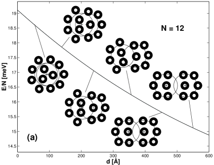
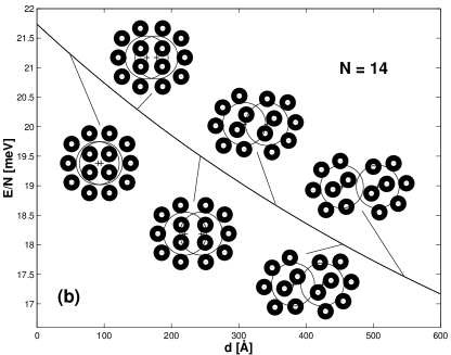
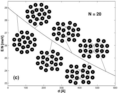
Figure 4: (a) - (c) Ground state electron configurations along $E(d)$ curve for $N=12,14$ and $20$.

For other electron numbers besides the reported $N=6,8,16,17,18,19$ we do not observe discontinuous structural transitions in the electron configuration as the distance between the two atoms is increased. A few examples of continuous electron configuration changes are shown in Fig. 4. For $N=12$ the (3,9) configuration transforms continuously to resemble the (6),(1,5)^∗ two-atom configuration. Between $200$ Å and $450$ Å the row of electrons pushes itself forward when the atoms move apart, resulting in the symmetric configuration (1,5)^∗,(1,5)^∗. For $N=14$ the electron configuration follows the separation of atoms in a symmetrical form, but after $d=250$ Å both sides start to twist towards the (1,6),(1,6) two-atom configuration. For $N=20$ the transformation is hard to describe, but it is continuous. The three distinct metastable states at $d=0$ and $200$ Å, seen in Table 1, never change to a ground state and vanish at other distances.

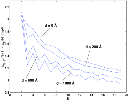
Figure 5: Change in the chemical potential ($E_{N+1}/(N+1)-E_{N}/N$) at $d=0,200,600$ and $1000$ Å.

The changes in energy per particle of the ground states at the four studied distances as a function of $N$ are shown in Fig. 5. At $d=$ 0 there are small troughs at $N=3,6,10$ and $17$, at adding the fourth, seventh, eleventh and eighteenth particle. Moving to greater distances between the atoms, the change in the chemical potential is clearly peaked. Going to an odd number of particles increases the chemical potential much more than going to an even number of particles. Interesting is the intermediate distance of $d=$ 200 Å where this trend is observed for $N=2,3,4$ and $9,10,11$, but otherwise the curve shows no clear structure and does not strictly follow the shape of the $d=0$ Å curve either.

IV Discussion

At $d=0$ (single artificial atom) our results are in agreement with other Monte Carlo (MC) and molecular dynamics (MD) studies with parabolic confinement and pure Coulomb interaction. Bolton and Rössler (1993); Bedanov and Peeters (1994); Schweigert and Peeters (1995); Lai and I (1999); Date et al. (1998); Kong et al. (2001) However, for $N=17$ Bolton et al.  Bolton and Rössler (1993) obtain the (1,5,11) configuration instead of (1,6,10) which our and other calculationsBedanov and Peeters (1994); Schweigert and Peeters (1995); Lai and I (1999); Kong et al. (2001) predict. Ref. Bolton and Rössler, 1993 may contain an error since in a later work by BoltonBolton (1994) the configuration for $N=17$ was reported to be (1,6,10). There is also a difference for $N=21$ in Ref. Bolton and Rössler, 1993 which was later corrected.Bolton (1994)

Besides calculating the ground state configurations Kong et al.  Kong et al. (2001) also examined metastable states for $N=1-40$. Our results are in agreement (we calculated configurations only for $N\leq 20$) both in ground and metastable states except that for $N=18$ Kong et al. found two metastable states whereas we see only one. In addition to the (1,6,11) and (1,7,10) they also obtain (6,12) as a metastable state. We repeated the simulation with 3000 independent test runs, but were still unable to find the (6,12) configuration.

We can conclude that different calculations for the $r^{2}$ confinement and $1/r$ interaction potential are in good general agreement. The few experiments on charged particles trapped in 2D as well as calculations with different forms of interaction and confinement potentials reveal also different configurations for the cluster patterns. The interaction between the particles could be logarithmic, which is the case with infinite charged lines moving in 2D (vortex lines etc.) or perhaps Yukawa type with a strong but short-range repulsion (screened Coulomb interaction). The form of the confinement is usually chosen to be parabolic (Lai and I Lai and I (1999) tested also a steeper confinement with $r^{4}$ contribution). However, for the question whether the potential in experiments with clusters is parabolic there is no clear answer. Therefore it is not surprising that the experiments and also calculations with different functional forms of interaction and confinement result in different cluster patterns.

Lai and I Lai and I (1999) calculated and summarised the configuration patterns with different interactions and tested also $r^{4}$ contribution to the confinement and compared the results to dust particle experiments. Juan et al. (1998) Saint Jean et al.  Saint Jean et al. (2001) measured the configurations with electrostatically interacting charged balls of millimeter size moving on a plane conductor. They made a comparison with simulations and quite surprisingly found the best agreement with a relatively old simulation with vortex lines in a superfluidCampbell and Ziff (1979) with logarithmic interaction, which again was not in agreement with the dust particle experimentsJuan et al. (1998) nor with the purely logarithmic interaction used by Lai and I. Lai and I (1999) Despite the differences there are some particle numbers where the configuration seems to be the same regardless of the experiment or functional form of the interaction or confinement. These particle numbers are $N=3,4,5,7,10,12,14,19$.

Partoens et al. Partoens et al. (1997) examined the ground states of even number of classical electrons evenly distributed in two vertically coupled artificial atoms as a function of the distance between the atoms. As in our study of laterally coupled atoms discontinuous transitions between configurations occur as a function of the distance $d$. The difference is that for vertically coupled atoms one can see intuitively that transitions should occur between $d=0$ and $d\rightarrow\infty$ whereas in laterally coupled atoms the configurations can be pulled apart with some $N$ without qualitative (discontinuous) changes in the electron configurations. For vertically coupled atoms discontinuous transitions (first order with respect to energy) in electron configurations are observed for all even $N\leq 20$ whereas for laterally coupled atoms we see also purely continuous changes as $d\rightarrow\infty$.

To summarise, we have calculated ground and metastable state configurations of classical point charges confined in two dimensions with two laterally coupled parabolic potential wells. Ground and metastable electron configurations were studied as a function of the distance between the atoms and discontinuous (in $\partial E/\partial d$) transitions in the ground state configurations were observed for particle numbers $N=6,8,11,16,17,18,19$. The configurations of purely classical electrons in laterally coupled two-minima potential have an interesting and complex spectrum as the distance between the minima is changed.