Quantum Brownian motion in ratchet potentials

Abstract

We investigate the dynamics of quantum particles in a ratchet potential subject to an ac force field. We develop a perturbative approach for weak ratchet potentials and force fields. Within this approach, we obtain an analytic description of dc current rectification and current reversals. Transport characteristics for various limiting cases – such as the classical limit, limit of high or low frequencies, and/or high temperatures – are derived explicitly. To gain insight into the intricate dependence of the rectified current on the relevant parameters, we identify characteristic scales and obtain the response of the ratchet system in terms of scaling functions. We pay a special attention to inertial effects and show that they are often relevant, for example, at high temperatures. We find that the high temperature decay of the rectified current follows an algebraic law with a non-trivial exponent, $j\propto T^{-17/6}$.

I Introduction

Ratchets have attracted a considerable recent interest because of their paradigmatic role as microscopic transport devices (for review articles, see e.g. Refs. Astumian, 1997; Bier, 1997; Reimann, ). Applications range from microscale electronics – including the photogalvanic effect,Belinicher and Sturman (1980) transport in quantum dotsLinke et al. (1998a, b) and antidot arraysLorke et al. (1998) – over Josephson junctions Zapata et al. (1996); Falo et al. (1999); Weiss et al. (2000); Goldobin et al. (2001) and vortex matterOlson et al. to cell biology.Jülicher et al. (1997) At the same time, ratchets are of fundamental theoretical interest since they represent one of the simplest nonequilibrium systems.

The analysis of ratchet systems reaches back quite some time before Feynman drew the attention of a wide audience to such systems in his lectures where he discussed the possibility to employ ratchets as heat engines.Feynman et al. (1963) Subsequently, researches in ratchets have been progressing steadily, in parallel in different scientific communities, until the explosive outburst in theoretical and experimental interest in the 1990s not (a) had occurred.

In this paper, we report on the analytic progress in the study of the so called tilting ratchets, where the combination of an asymmetric static potential with an unbiased ac force and a coupling to a heat bath leads to current rectification. Past theoretical studies of this ratchet type focused on the classical massless case Magnasco (1993); Bartussek et al. (1994) and have revealed the current reversal phenomenon, i.e., the possibility that the direction of the rectified current reverses its direction when model parameters such as the frequency or amplitude of the ac current are changed. The inclusion of a finite mass of the particles has shown that it may give rise even to multiple current reversals.Jung et al. (1996) Further extensions accounted for the quantum nature of particles and of the bath. Quantum fluctuations were found to provide an additional source of current reversals.Reimann et al. (1997); Yukawa et al. (1997); Tatara et al. (1998)

In essence, the direction and amplitude of the current turned out to be very sensitive to the various system parameters. While this dependence makes ratchets valuable for applications – such as devices that can separate particles of different species – it still lacks a satisfying theoretical understanding. Analytic approaches can give insight into this problem. However, even the single-particle problem is already so complex that analytic approaches can be advanced only in limiting cases, such as the adiabatic limitReimann et al. (1997) or the deterministic limit.Jung et al. (1996); Mateos (2000)

In our paper we develop a perturbative approach valid for weak ratchet potentials and weak driving forces, which covers a wide range of practical applications. Within this perturbative approach we are able to capture all prominent phenomena including multiple current reversals. This approach provides a unified framework for deriving and understanding the dependence of the rectified current on the particle mass, temperature, friction coefficient, and frequency of the driving force. We pay particular attention to the role of inertial effects and show that they lead to a substantial current enhancement even in the high-temperature limit.

In Sec. II we specify the model and establish a path-integral formulation as analytic framework. The perturbative scheme is developed in Sec. III. In Sec. IV we briefly demonstrate that the linear mobility can be conveniently obtained from this approach and that results for special cases known in the literature are reproduced. However, ratchet effects can be obtained only in nonlinear response. The leading nonlinear mobility is calculated and evaluated for various limiting cases in Sec. V. We conclude with a discussion of our approach and results in Sec. VI. Technical details of our calculations are presented in appendices.

II Model

We consider a quantum particle of the mass $m$ in a stationary ratchet potential $U(x)$. In addition, we impose an ac driving force $F(t)$ which is chosen to be unbiased, i.e., to vanish upon time averaging. Following Caldeira and Leggett,Caldeira and Leggett (1983) we couple the particle linearly to a bath of harmonic oscillators at temperature $T$. This bath simultaneously provides friction and a fluctuating force for the particle. For simplicity, we assume a linear spectral distribution of these oscillators, giving rise to Ohmic dissipation. In the classical limit, the particle coordinate $x(t)$ follows the equation of motion

$$m\ddot{x}(t)=-U^{\prime}(x(t))+F(t)-\eta\dot{x}(t)+\xi(t)$$ (1)

with a friction coefficient $\eta$ and a Gaussian thermal noise $\xi(t)$ obeying

$$\langle\xi(t)\rangle=0,\quad\langle\xi(t)\xi(t^{\prime})\rangle=2\eta T\delta(t-t^{\prime}).$$ (2)

To account for the quantum nature of the particle and of the bath, we follow the analysis of quantum Brownian motion by Fisher and ZwergerFisher and Zwerger (1985); Zwerger (1987) who studied the case of a sinusoidal potential and a dc driving force.

The rectified particle velocity $V$ can be determined from the average particle coordinate $X(t)$ via

$$V \equiv \lim_{t\to\infty}\frac{1}{t}X(t),$$ (3a)

$$X(t) \equiv \int dx\ x\ P(t,x),$$ (3b)

where $P(t,x)$ is the probability distribution for the particle position at time $t$. This distribution is related to the reduced density matrix operator ${\hat{\rho}}(t)$ (after the bath degrees of freedom are traced out) by

$$P(t,x)=\langle x|{\hat{\rho}}(t)|x\rangle.$$ (4)

[We use the Dirac notation, where $\langle x^{+}|{\hat{\rho}}(t)|x^{-}\rangle$ is the density matrix in position representation.]

The dynamics of this density matrix is most conveniently treated in the Feynman-Vernon path integral representation.Feynman and Vernon (1963); Kleinert (1995) The time evolution of the density matrix from some initial time $t_{\textrm{i}}$ to a final time $t_{\textrm{f}}$ is given by

$$\langle x^{+}_{\textrm{f}}|{\hat{\rho}}(t_{\textrm{f}})|x^{-}_{\textrm{f}}\rangle = \iint dx^{+}_{\textrm{i}}dx^{-}_{\textrm{i}}J(t_{\textrm{f}},x_{\textrm{f}}^{+},x_{\textrm{f}}^{-};t_{\textrm{i}},x_{\textrm{i}}^{+},x_{\textrm{i}}^{-})$$ (5a)

$$\times\langle x^{+}_{\textrm{i}}|{\hat{\rho}}(t_{\textrm{i}})|x^{-}_{\textrm{i}}\rangle$$

with the kernel

$$J(t_{\textrm{f}},x_{\textrm{f}}^{+},x_{\textrm{f}}^{-};t_{\textrm{i}},x_{\textrm{i}}^{+},x_{\textrm{i}}^{-})=\int Dx\ Dy\ e^{-S}$$ (5b)

being a double path integral over all trajectories $x(t)$ and $y(t)$ with the boundary conditionsnot (b)

$$x(t_{{\textrm{i}},{\textrm{f}}})=\frac{1}{2}(x_{{\textrm{i}},{\textrm{f}}}^{+}+x_{{\textrm{i}},{\textrm{f}}}^{-}),\quad y(t_{{\textrm{i}},{\textrm{f}}})=\frac{1}{\hbar}(x_{{\textrm{i}},{\textrm{f}}}^{+}-x_{{\textrm{i}},{\textrm{f}}}^{-}).$$ (6)

The path integral involves the effective action

$$S = S_{0}+S_{1},$$ (7a)

$$S_{0} = \frac{1}{2}\iint dtdt^{\prime}\ y(t)K(t-t^{\prime})y(t^{\prime})$$ (7b)

$$+i\int dt\ y(t)[m\ddot{x}(t)+\eta\dot{x}(t)],$$

$$S_{1} = i\int dt\Big{[}\sum_{s}\frac{1}{2s}U(x(t)+sy(t))-y(t)F(t)\Big{]},$$ (7c)

with all time integrals running from $t_{\textrm{i}}$ to $t_{\textrm{f}}$. For notational convenience, the usual contribution $U(x^{+}(t))-U(x^{-}(t))$ is written as a sum over the spin-like variable $s=\pm\hbar/2$ which, however, does not have the meaning of a physical spin.

The effective action (7) includes already the average over the bath degrees of freedom. This average leads to an integral kernel $K(t)$ which reads in Fourier representationnot (c) (we set $k_{\rm B}=1$)

$$K(\omega)={\eta\hbar\omega}\textrm{ coth }\frac{\hbar\omega}{2T}.$$ (8)

In the classical limit, $K(\omega)=2\eta T$ reproduces the correlator (2). For $T=0$, $K(\omega)=\eta\hbar|\omega|$ represents a kernel that is highly nonlocal in time representation.

The model has a large number of parameters: the particle mass $m$ and the friction coefficient $\eta$, then $\hbar$ and $T$ as a measure of the strength of quantum and thermal fluctuations. Further parameters are implicit in $U(x)$ and $F(t)$. The potential can be represented by a Fourier series

$$U(x)=\sum_{q}U_{q}\ e^{iqx}$$ (9)

with amplitudes $U_{q}$ for wave vectors $q$. For periodic potentials with a period $a$, the wave vectors are

$$q=n\frac{2\pi}{a}$$ (10)

with integer $n$.

In analogy to $U$, the ac drive is represented as

$$F(t)=\sum_{\omega}F_{\omega}\ e^{-i\omega t}$$ (11)

with $F_{0}=0$ since the force is assumed to be unbiased on time average. For a periodic drive with period $t_{F}$, the frequencies $\omega$ are integer multiples of the basic frequency $2\pi/t_{F}$. Although we assume here periodicity of $U$ and $F$, a generalization to random $U$ and $F$ is straightforward and will be discussed in the end of this paper.

III Perturbative approach

The definition (3) of the velocity has the drawback that one has to calculate $X(t)$ as the expectation value of the final position in an ensemble of forward-backward paths of a finite length $t_{\textrm{f}}-t_{\textrm{i}}$. In order to avoid technical complications related to boundary effects, we relate the average velocity to an expectation value at an intermediate time $t$ which can be kept fixed while the limit $t_{\textrm{i}}\to-\infty$ and $t_{\textrm{f}}\to\infty$ is been taken.

Consider the “partition sum”

$$Z = \int dx_{\textrm{f}}\iint dx^{+}_{\textrm{i}}dx^{-}_{\textrm{i}}J(t_{\textrm{f}},x_{\textrm{f}},x_{\textrm{f}};t_{\textrm{i}},x_{\textrm{i}}^{+},x_{\textrm{i}}^{-})$$ (12)

$$\times\langle x^{+}_{\textrm{i}}|{\hat{\rho}}(t_{\textrm{i}})|x^{-}_{\textrm{i}}\rangle$$

of all forward-backward paths between $t_{\textrm{i}}$ and $t_{\textrm{f}}$. It is normalized to $Z=1$ since it is the trace of the density matrix at $t_{\textrm{f}}$. We define

$$V(t)\equiv\langle\dot{x}(t)\rangle$$ (13)

as expectation value in the ensemble $Z$ of fluctuating paths. In this definition, we can take the limit $t_{\textrm{i}}\to-\infty$ and $t_{\textrm{f}}\to\infty$ right away. In the absence of a nonequilibrium driving force and due to the presence of dissipation, $V(t)$ would vanish after an initial relaxation for every possible initial density matrix ${\hat{\rho}}(t_{\textrm{i}})$. In the presence of the driving force and in the limit $t_{\textrm{i}}\to-\infty$, $V(t)$ will be determined uniquely by $F(t)$ and independently of the initial state.

Although we strictly follow the definition of Fisher and ZwergerFisher and Zwerger (1985); Zwerger (1987) in the path integral formulation of the problem, we differ in the definition of the average velocity. We argue in appendix A that, in the long time limit, the time average of the velocity $V(t)$ coincides with the earlier definition (3) in combination with (4) and (5). We find the expectation value $V(t)$ to be a convenient quantity for the subsequent perturbative evaluation.

III.1 Perturbative expansion

To make analytic progress, we consider $F$ as small and calculate the nonlinear dynamic response of the velocity to the driving force,

$$V(t) = \int dt^{\prime}\mu_{1}(t-t^{\prime})F(t^{\prime})$$ (14)

$$+\frac{1}{2!}\iint dt^{\prime}dt^{\prime\prime}\mu_{2}(t-t^{\prime},t-t^{\prime\prime})F(t^{\prime})F(t^{\prime\prime})$$

$$+O(F^{3}).$$

The mobilities $\mu_{m}$ can be expressed conveniently as expectation values in the path ensemble using the partition sum as generating functional,

$$\mu_{1}(t-t^{\prime}) = \left.\frac{\delta V(t)}{\delta F(t^{\prime})}\right|_{F=0}$$ (15a)

$$= \left.\langle\dot{x}(t)iy(t^{\prime})\rangle\right|_{F=0},$$

$$\mu_{2}(t-t^{\prime},t-t^{\prime\prime}) = \left.\frac{\delta^{2}V(t)}{\delta F(t^{\prime})\delta F(t^{\prime\prime})}\right|_{F=0}$$ (15b)

$$= \left.\langle\dot{x}(t)iy(t^{\prime})iy(t^{\prime\prime})\rangle\right|_{F=0}.$$

The generalization to higher order mobilities is straightforward. The expectation values now refer to the equilibrium system in the absence of the driving force.

After Fourier transformation, Eq. (14) reads

$$V_{\omega} = \mu_{1}(\omega)F_{\omega}+\frac{1}{2!}\sum_{\omega^{\prime}\omega^{\prime\prime}}\mu_{2}(\omega^{\prime},\omega^{\prime\prime})F_{\omega^{\prime}}F_{\omega^{\prime\prime}}\delta_{\omega,\omega^{\prime}+\omega^{\prime\prime}}$$ (16)

$$+O(F^{3}).$$

The rectified current is given by the time-average (zero frequency component) of the velocity,

$$V_{0}=\frac{1}{2}\sum_{\omega}\mu_{2}(-\omega,\omega)F_{-\omega}F_{\omega}+O(F^{3}).$$ (17)

Since the driving force is unbiased, $F_{0}=0$, current rectification cannot be obtained in linear response. Rather, ratchet effects require frequency mixing which is present only in nonlinear response. For weak $F$ the leading ratchet effect will be determined by $\mu_{2}$.

If the driving force has the symmetry

$$F(t)=-F(t-t_{0})$$ (18)

for some time $t_{0}$ (for example, if $F$ is monochromatic), the rectified velocity will be invariant under the transformation $F(t)\to F(t-t_{0})=-F(t)$. Then the contributions to the rectified current from all mobilities $\mu_{m}$ with odd $m$ must vanish.

Although the calculation of these mobilities is already much simpler than a closed calculation of $V(t)$, it still cannot be performed analytically for general potentials. Therefore, we employ a second expansion in $U$, utilizing the weakness of the potential.

The mobilities, which, according to Eqs. (15), are the equilibrium expectation values $\mu_{m}=\left.\langle{\mathcal{O}}_{m}\rangle\right|_{F=0}$ of observables ${\mathcal{O}}_{m}\equiv\dot{x}(t)iy(t^{\prime})\cdots iy(t^{(m)})$, will be calculated perturbatively in the potential using the expansionFisher and Zwerger (1985); Zwerger (1987)

$$\left.e^{-S_{1}}\right|_{F=0}=\sum_{n=0}^{\infty}\frac{1}{n!}\left\{\int dt\sum_{s,q}\frac{U_{q}}{2is}e^{iq[x(t)+sy(t)]}\right\}^{n}.$$ (19)

We thus can write

$$\mu_{m}=\sum_{n=0}^{\infty}\mu_{m}^{(n)}$$ (20)

with

$$\mu_{m}^{(n)} = \frac{1}{n!}\sum_{{s_{1}},q_{1},\cdots,{s_{n}},q_{n}}\prod_{j=1}^{n}\frac{U_{q_{j}}}{2i{s_{j}}}\int dt_{1}\cdots\int dt_{n}$$ (21)

$$\times\Big{\langle}{\mathcal{O}}_{m}\exp\Big{(}{i\sum_{j=1}^{n}q_{j}[x(t_{j})+s_{j}y(t_{j})]}\Big{)}\Big{\rangle}_{0}$$

where the average $\langle\cdots\rangle_{0}$ is governed by the “free” action $S_{0}$ defined by Eq. (7b). Since $S_{0}$ is Gaussian, the averages can be performed straightforwardly using Wick’s theorem.

III.2 Free theory

For these averages it is important to know the correlations of the free theory. In Fourier representation, one easily finds

$$\langle x(\omega^{\prime})x(\omega^{\prime\prime})\rangle_{0} = C(\omega^{\prime})\delta(\omega^{\prime}+\omega^{\prime\prime}),$$ (22a)

$$\langle x(\omega^{\prime})iy(\omega^{\prime\prime})\rangle_{0} = G(\omega^{\prime})\delta(\omega^{\prime}+\omega^{\prime\prime}),$$ (22b)

$$\langle y(\omega^{\prime})y(\omega^{\prime\prime})\rangle_{0} = 0,$$ (22c)

with the response and correlation functions

$$G(\omega) = -\frac{1}{i\eta\omega+m\omega^{2}-0^{+}},$$ (23a)

$$C(\omega) = \frac{K(\omega)}{\eta^{2}\omega^{2}+m^{2}\omega^{4}}.$$ (23b)

To calculate the nonlinear mobilities, one has to use the retarded response function which is in time representation

$$G(t) = \langle x(t)iy(0)\rangle_{0}=\frac{1}{\eta}[1-e^{-\gamma t}]\Theta(t)$$ (24)

with a relaxation rate defined by

$$\gamma\equiv\frac{\eta}{m}.$$ (25)

Causality of response

$$G(t)=0\textrm{ for }t\leq 0$$ (26)

is reflected by the Heaviside step function $\Theta(t)$ in (24). Note that $\langle x^{2}(t)\rangle=\infty$ since the free system is translation invariant and the particle spreads diffusively (subdiffusively for $T=0$) over the entire space. Therefore, $C(t)$ is not a well defined quantity. Instead, the displacement function

$$W(t) \equiv \frac{1}{2}\langle[x(t)-x(0)]^{2}\rangle_{0}$$ (27a)

$$= \int\frac{d\omega}{2\pi}[1-\cos(\omega t)]C(\omega)$$ (27b)

captures all information about the particle (sub)diffusion. This quantity will play a central role in perturbation theory. Unfortunately, it can be calculated explicitly only in limiting cases:

$$W(t) = \frac{T}{\eta\gamma}[\gamma|t|+e^{-\gamma|t|}-1]\quad\textrm{ for }\hbar=0,$$ (27c)

$$W(t) \sim \frac{\hbar}{\pi\eta}\ln\gamma|t|\quad\textrm{ for }T=0.$$ (27d)

For semiquantitative purposes,

$$W(t)\approx\frac{T}{\eta\gamma}[\gamma|t|+e^{-\gamma|t|}-1]+\frac{\hbar}{2\pi\eta}\ln[1+(\gamma t)^{2}]$$ (27e)

is a good interpolation over the whole parameter range.

We conclude this subsection by pointing out some key features of the response and displacement function. For $\hbar=0$, $G$ and $W$ are related through the fluctuation-dissipation relation

$$TG(t)=\dot{W}(t)\Theta(t).$$ (28)

In the quantum case with $T=0$, $W(t)$ diverges for all $t$ in the limit $m\to 0$.

III.3 Characteristic scales

Before we move on to a further evaluation of the path integral, we pause for a moment to fix the relevant time, length, and energy scales of our problem. From the response function of our problem we can identify the typical relaxation time

$$t_{\textrm{rel}}={\frac{1}{\gamma}}=\frac{m}{\eta}.$$ (29)

Rewriting the displacement correlation function $W(t)=\ell^{2}\hat{W}(t/t_{\textrm{rel}})$ in terms of the dimensionless function $\hat{W}$ of the dimensionless argument $t/t_{\textrm{rel}}$, we identify from Eqs. (27) the diffusion lengths $\ell$ for the thermal and the quantum case,

$$\ell_{\textrm{th}}^{2}=\frac{Tm}{\eta^{2}},\quad\ell_{\textrm{qu}}^{2}=\frac{\hbar}{\eta}.$$ (30)

The de-Broglie wave length

$$\lambda^{2}=\frac{2\pi\hbar^{2}}{mT}=2\pi\frac{\ell_{\textrm{qu}}^{4}}{\ell_{\textrm{th}}^{2}}$$ (31)

is a related further characteristic scale for the particle in the absence of dissipation.

Alternatively to Eqs. (30), we can associate with thermal and quantum fluctuations a characteristic energies $E=\eta^{2}\ell^{2}/m$,

$$E_{\textrm{th}}=T,\quad E_{\textrm{qu}}=\hbar\gamma.$$ (32)

The potential and driving force – which act as probes to the free particle – define the space period $a$, time period $t_{F}$, and amplitudes

$${\mathcal{U}}=2|U_{q}|,\quad{\mathcal{F}}=2|F_{\omega}|,$$ (33)

defined by the lowest harmonic modes $q$ and $\omega$. In the case of random $U$ or $F$, the periods would be replaced by a correlation length or time and the amplitudes by variances.

In terms of these scales, a necessary requirement for the validity of the perturbative approach is that external probes must be weak in comparison to the internal fluctuations, i.e.,

$${\mathcal{U}},a{\mathcal{F}}\ll\max(E_{\textrm{th}},E_{\textrm{qu}}).$$ (34)

These scales will also determine the location of the phenomena under consideration, as we will discuss later on. However, as we recall by calculating the linear response mobility, th condition (34) is not sufficient for the validity of perturbative results.

In the subsequent calculations it is convenient to use dimensionless quantities. It is natural to choose as time scale, or $\gamma$ as frequency scale. The generic length scale is the potential period $a$. The ratios of $\ell_{\textrm{th}}^{2}$ and $\ell_{\textrm{qu}}^{2}$ to $a^{2}$ provide a natural measure for the strength of thermal and quantum fluctuations. Hence we define

$${\hat{t}}\equiv\gamma t,\ \ {\hat{\omega}}\equiv\frac{\omega}{\gamma},\ \ \hat{q}_{j}\equiv aq_{j},\ \ \hat{\hbar}\equiv\frac{\hbar}{\eta a^{2}},\ \ \hat{T}\equiv\frac{Tm}{\eta^{2}a^{2}}.$$ (35)

as dimensionless quantities.

III.4 Mobilities

In Eq. (21), the mobilities $\mu_{m}^{(n)}$ are determined by expectation values which can be calculated conveniently from a generating functional. We define

$${\mathcal{Z}}\equiv\Big{\langle}\exp\Big{(}i\int d\tau[\rho(\tau)x(\tau)+\sigma(\tau)y(\tau)]\Big{)}\Big{\rangle}_{0}$$ (36)

as functional of auxiliary fields $\rho(\tau)$ and $\sigma(\tau)$. $\tau$ is a real time variable and we will be distinguishing it from $t$ only for bookkeeping purposes. The averages determining the mobilities $\mu_{m}^{(n)}$ can be then represented as functional derivatives

$$\Big{\langle}{\mathcal{O}}_{m}\exp\Big{(}{i\sum_{j=1}^{n}q_{j}[x(t_{j})+s_{j}y(t_{j})]}\Big{)}\Big{\rangle}_{0}=$$

$$-i\frac{d}{dt}\frac{\delta^{(m+1)}}{\delta\rho(t)\delta\sigma(t^{\prime})\cdots\delta\sigma(t^{(m)})}{\mathcal{Z}},$$ (37)

where one has to identify

$$\rho(\tau) = \sum_{j=1}^{n}q_{j}\delta(\tau-t_{j}),$$ (38a)

$$\sigma(\tau) = \sum_{j=1}^{n}q_{j}s_{j}\delta(\tau-t_{j}),$$ (38b)

after performing the functional derivatives. Using the results of the previous subsection, the generating functional can be expressed as

$${\mathcal{Z}} = \exp\bigg{(}\iint d{\tau_{1}}d{\tau_{2}}\Big{[}-\frac{1}{2}\rho({\tau_{1}})C({\tau_{1}}-{\tau_{2}})\rho({\tau_{2}})$$ (39)

$$+i\rho({\tau_{1}})G({\tau_{1}}-{\tau_{2}})\sigma({\tau_{2}})\Big{]}\bigg{)}.$$

As mentioned previously, $C(t)$ is divergent. This implies that ${\mathcal{Z}}=0$ if $\int d\tau\rho(\tau)=\sum_{j}q_{j}\neq 0$. Therefore, ${\mathcal{Z}}$ can be nonvanishing only if the “momentum conservation” $\sum_{j}q_{j}=0$ is satisfied. In this case one may rewrite

$${\mathcal{Z}} = \exp\bigg{(}\iint d{\tau_{1}}d{\tau_{2}}\Big{[}\frac{1}{2}\rho({\tau_{1}})W({\tau_{1}}-{\tau_{2}})\rho({\tau_{2}})$$ (40)

$$+i\rho({\tau_{1}})G({\tau_{1}}-{\tau_{2}})\sigma({\tau_{2}})\Big{]}\bigg{)}\delta_{\{q\}}.$$

Hereby, we introduce the abbreviation $\delta_{\{q\}}\equiv\delta_{\sum q_{j},0}$. The subsequent calculations of the mobilities are based on this generating functional. For later convenience, we combine Eqs. (21), (37), and (40) to our master formula

$$\mu_{m}^{(n)}(t-t^{\prime},t-t^{\prime\prime},\cdots,t-t^{(n)}) = -i\frac{d}{dt}\frac{1}{n!}\sum_{{s_{1}},q_{1},\cdots,{s_{n}},q_{n}}\delta_{\{q\}}\prod_{j=1}^{n}\frac{U_{q_{j}}}{2i{s_{j}}}\int dt_{1}\cdots\int dt_{n}\frac{\delta^{(m+1)}}{\delta\rho(t)\delta\sigma(t^{\prime})\cdots\delta\sigma(t^{(m)})}$$ (41)

$$\times\exp\bigg{(}\iint d{\tau_{1}}d{\tau_{2}}\Big{[}\frac{1}{2}\rho({\tau_{1}})W({\tau_{1}}-{\tau_{2}})\rho({\tau_{2}})+i\rho({\tau_{1}})G({\tau_{1}}-{\tau_{2}})\sigma({\tau_{2}})\Big{]}\bigg{)}.$$

Thereby, the substitution (38) has to be made after all functional derivatives are taken. Momentum conservation implies that all mobilities vanish for no $n=1$. For $n=2$ and even $m$ the mobilities vanish since the contributions to the sum in the right hand side of Eq. (41) are odd in $\{q\}$. We have noted already above, that no contribution to the rectified current can arise from $\mu_{m}$ with odd $m$ and arbitrary $n$ if the driving force obeys the symmetry (18). In this case, up to fifth order in $F$ and $U$, the only contribution comes from $\mu_{2}^{(3)}$.

After we have determined the generating functional ${\mathcal{Z}}$ for the mobilities in the previous section, we now turn to the evaluation of the lowest order mobilities of interest.

IV Linear mobility $\mu_{1}$

Although we do not expect ratchet effects from linear response, it is instructive to calculate $\mu_{1}$ in order $U^{2}$ to verify that the present calculation of the mobility reproduces that results of Fisher and ZwergerFisher and Zwerger (1985); Zwerger (1987) for static $F$ and sinusoidal $U$ (i.e., for this purpose we include the amplitude $F_{0}$ in our consideration).

IV.1 Leading orders

To zeroth order in $U$, it is obvious that

$$\mu_{1}^{(0)}(t-t^{\prime})=\dot{G}(t-t^{\prime}).$$ (42)

To first order,

$$\mu_{1}^{(1)}(t-t^{\prime})=0$$ (43)

since the momentum conservation mentioned above cannot be satisfied (strictly speaking, it is satisfied for the mode $q=0$ which, however, does not enter the dynamics).

To second order, a straightforward calculation (see appendix B) leads to

$$\mu_{1}^{(2)}(\omega) = i\omega G^{2}(\omega)\sum_{q}q^{2}|U_{q}|^{2}\Delta B_{-q,q}^{(2)}(\omega)$$ (44)

with

$$\Delta B_{-q,q}^{(2)}(\omega) \equiv B_{-q,q}^{(2)}(\omega=0)-B_{-q,q}^{(2)}(\omega),$$ (45a)

$$B_{q_{1},q_{2}}^{(2)}(t) = \frac{2}{\hbar}\sin[\frac{\hbar}{2}q_{1}^{2}G(t)]e^{-q_{1}^{2}W(t)}\delta_{q_{1}+q_{2},0}.$$ (45b)

In the last expression, the sine has a nonunique sign for

$$\pi<\frac{\hbar}{2}q^{2}G(\infty)=\frac{\hbar q^{2}}{2\eta}$$ (46)

reflecting quantum interferences of particle trajectories.

We briefly discuss interesting limiting cases of $\mu_{1}^{(2)}$ for which we will also examine the ratchet effect later on.

IV.2 Classical limit

In a classical limit, $\hbar\to 0$, both the overdamped and underdamped cases are understood fairly well.Ambegaokar and Halperin (1969a, b); Ivanchenko and Zil’berman (1969); Nozières and Iche (1979) In the present perturbative approach, the fluctuation-dissipation theorem (28) allows for the simplification

$$B_{q_{1},q_{2}}^{(2)}(t)=-\frac{1}{T}\frac{d}{dt}e^{-q_{1}^{2}W(t)}\Theta(t)\delta_{q_{1}+q_{2},0}.$$ (47)

In this case, the Fourier transformation can be performed analytically,

$$\Delta B^{(2)}_{-q,q}(\omega) = -\frac{i\omega}{T}\int_{0}^{\infty}dt\ e^{i\omega t}e^{-q^{2}W(t)}$$ (48a)

$$= -\frac{i{\hat{\omega}}}{T}e^{{\hat{\nu}}_{q}}{\hat{\nu}}_{q}^{-({\hat{\nu}}_{q}-i{\hat{\omega}})}\gamma({\hat{\nu}}_{q}-i{\hat{\omega}},{\hat{\nu}}_{q}),$$ (48b)

with $\gamma(\cdot,\cdot)$ the incomplete gamma function (to be distinguished from the parameter $\gamma$). We introduced the dimensionless frequency

$${\hat{\nu}}_{q}\equiv\ell_{\textrm{th}}^{2}q^{2}=\frac{Tmq^{2}}{\eta^{2}}$$ (49)

related to the thermal diffusion time over a distance $1/q$ via $W(t_{\textrm{rel}}/{\hat{\nu}}_{q})=q^{-2}$. The insertion of expression (48b) into Eq. (44) yields an explicit analytic expression for the classical linear response mobility at finite frequencies,

$$\mu_{1}^{(2)}(\omega) = -\frac{1}{\eta}\frac{1}{(1-i{\hat{\omega}})^{2}}$$ (50)

$$\times \sum_{q}\frac{|U_{q}|^{2}}{T^{2}}e^{{\hat{\nu}}_{q}}{\hat{\nu}}_{q}^{1-({\hat{\nu}}_{q}-i{\hat{\omega}})}\gamma({\hat{\nu}}_{q}-i{\hat{\omega}},{\hat{\nu}}_{q})$$

which reproduces Eq. (4.11) of Ref. Fisher and Zwerger, 1985 for the special case of sinusoidal $U$ and $\omega=0$.

In the massless (overdamped) limit $m\to 0$, where $B$ can be easily Fourier transformed, this simplifies to

$$\mu_{1}^{(2)}(\omega) = -\frac{1}{\eta}\frac{{\mathcal{U}}^{2}}{T^{2}}{\hat{\mu}}_{1}^{(2)}\left(\frac{\eta a^{2}\omega}{T}\right)$$ (51)

with a dimensionless scaling function

$${\hat{\mu}}_{1}^{(2)}(z) = \sum_{q}\frac{|U_{q}|^{2}}{{\mathcal{U}}^{2}}\frac{\hat{q}^{2}}{\hat{q}^{2}-iz}.$$ (52)

Thus, for $m=0$, the corrections to mobility decay proportional to $T^{-2}$ at high temperatures.

IV.3 Adiabatic limit

The adiabatic limit $\omega\to 0$ simplifies the calculation of $\Delta B_{-q,q}^{(2)}(\omega)$, resulting in

$$\mu_{1}^{(2)}(\omega=0) = -\frac{2}{\eta^{2}\hbar}\sum_{q}|U_{q}|^{2}q^{2}$$ (53)

$$\times\int_{0}^{\infty}dt\ t\ e^{-q^{2}W(t)}\sin[\frac{\hbar}{2}q^{2}G(t)]$$

which agrees with the linear response limiting case (4.18) of Ref. Fisher and Zwerger, 1985.

At $T=0$, the particle shows a remarkable localization transition due to the dissipative coupling.Schmid (1983); Fisher and Zwerger (1985) For strong coupling, the particle is localized in an arbitrarily weak potential, whereas it remains mobile for weak damping. This transition is reflected by the divergence of the mobility correction $\mu_{1}^{(2)}(\omega=0)$ due to a divergence of the time integral at large $t$. From the logarithmic asymptotics (27d) of $W(t)$ one can identify the location of the transition at $\alpha=1$ with

$$\alpha\equiv\frac{\eta a^{2}}{2\pi\hbar}=\frac{1}{2\pi\hat{\hbar}}.$$ (54)

Note that for $\alpha<1$ the inequality (46) is fulfilled for all wave vectors $q$, i.e. quantum interference effects suppress the contribution to $\mu_{1}^{(2)}$.

In the strong damping regime, the divergence of $\mu_{1}^{(2)}(\omega=0)$ signals the break-down of perturbation theory. Thus, at $T=0$ the condition $\alpha\ll 1$ should be added to the condition (34). This condition may be regarded also as a condition for the period of the potential (with localization for $a^{2}\leq 2\pi\ell_{\textrm{qu}}^{2}$).

In the perturbatively accessible regime of $\alpha<1$, Fisher and ZwergerFisher and Zwerger (1985) pointed out the interesting fact that the mobility is a nonmonotoneous function of temperature. At zero temperature, the particle has its free mobility. Weak thermal fluctuations ($T<T^{*}$) first reduce mobility (thermally resisted quantum tunneling), whereas strong thermal fluctuations increase mobility back to its free value (thermally assisted hopping). The crossover occurs for $\alpha\ll 1$ at the temperature

$$T^{*}\simeq\frac{\pi^{2}\hbar^{2}}{3ma^{2}}$$ (55)

at which the de-Broglie wave length is comparable to the potential period, $\lambda\simeq a$.

Before we continue to enter new territory, we wish to conclude this subsection by stressing that our approach successfully reproduces previous linear response results for $\omega=0$ and already provides additional insight into the frequency dependence.

V Nonlinear mobility $\mu_{2}$

The generating functional formalism presented above provides an efficient tool to calculate also higher order mobilities. Here, we focus on the lowest order of $\mu_{2}$ in $U$ contributing to current rectification.

V.1 Leading orders

To zeroth order,

$$\mu_{2}^{(0)}(t-t^{\prime},t-t^{\prime\prime})=\langle\dot{x}(t)iy(t^{\prime})iy(t^{\prime\prime})\rangle_{0}=0$$ (56)

vanishes since $S_{0}$ is invariant under the reflection $\{x,y\}\to\{-x,-y\}$. To first order,

$$\mu_{2}^{(1)}(t-t^{\prime},t-t^{\prime\prime})=0$$ (57)

vanishes again because momentum conservation cannot be satisfied. To second order,

$$\mu_{2}^{(2)}(t-t^{\prime},t-t^{\prime\prime})=0$$ (58)

according to the general statements following Eq. (41).

The general third order contribution $\mu_{2}^{(3)}(t-t^{\prime},t-t^{\prime\prime})$ is given by expression (90) calculated in appendix C. Since this expression is somewhat clumsy and since we are interested only in ratchet effects, we can restrict our considerations to

$$\mu_{2}^{(3)}(-\omega,\omega) = -\frac{i}{\eta}\frac{1}{\eta^{2}\omega^{2}+m^{2}\omega^{4}}\sum_{q_{1}q_{2}q_{3}}U_{q_{1}}U_{q_{2}}U_{q_{3}}q_{1}$$ (59)

$$\times\{q_{1}q_{2}[2B^{(3)}_{\{q\}}(0,0)-B^{(3)}_{\{q\}}(-\omega,0)-B^{(3)}_{\{q\}}(\omega,0)]$$

$$+q_{1}q_{3}[2B^{(3)}_{\{q\}}(0,0)-B^{(3)}_{\{q\}}(-\omega,-\omega)-B^{(3)}_{\{q\}}(\omega,\omega)]$$

$$+q_{2}q_{3}[2B^{(3)}_{\{q\}}(0,0)-B^{(3)}_{\{q\}}(0,-\omega)-B^{(3)}_{\{q\}}(0,\omega)]\}$$

with

$$B^{(3)}_{\{q\}}(t_{1}-t_{2},t_{2}-t_{3}) = \frac{2}{\hbar}\sin[\frac{\hbar}{2}q_{1}G_{12}q_{2}]\frac{2}{\hbar}\sin[\frac{\hbar}{2}(q_{1}G_{13}q_{3}+q_{2}G_{23}q_{3})]$$ (60)

$$\times\exp(q_{1}W_{12}q_{2}+q_{2}W_{23}q_{3}+q_{1}W_{13}q_{3})\delta_{q_{1}+q_{2}+q_{3},0}\Theta_{23}.$$

Note that $B^{(3)}_{\{q\}}$ is an implicit function of $\{q\}$ and invariant under $\{q\}\to-\{q\}$. Consequently, $\mu_{2}^{(3)}(-\omega,\omega)$ changes sign under a reflection $U_{q}\to U_{-q}$ which implies that the rectified velocity (17) vanishes for even potentials as it should. Examining the contribution from a set of wave vectors $\{q\}$ and its reflected set $-\{q\}$, one can recognize that $\mu_{2}^{(3)}(-\omega,\omega)$ is real and that it depends only on

$$\hat{U}^{(3)}_{\{q\}}\equiv\textrm{Im }\frac{U_{q_{1}}U_{q_{2}}U_{q_{3}}}{{\mathcal{U}}^{3}}.$$ (61)

(In order to obtain simple analytic expressions below, we find it most convenient to use momentum conservation to eliminate the sum over $q_{2}$.) In Eq. (59), the sum over the momenta can be restricted to $q_{j}\neq 0$ (in addition to momentum conservation) since $B^{(3)}_{\{q\}}$ vanishes otherwise (later on, these restrictions are referred to by $\sum^{\prime}$). Physically, it is clear that a constant shift of the potential cannot enter the dynamics of the particle.

Eq. (59) is our main result in general form. Further analytic progress is hampered by the absence of an analytic expression for $W(t)$. Nevertheless, further analytic progress is possible in various limiting cases.

Using the dimensionless quantities defined in Eqs. (35) we may reexpress Eq. (59) as

$$\mu_{2}^{(3)}(-\omega,\omega)=\frac{{\mathcal{U}}^{3}}{\eta^{3}a^{3}\hbar^{2}\gamma^{4}}{\hat{\mu}}_{2}^{(3)}(\hat{\hbar},\hat{T},{\hat{\omega}})$$ (62)

with ${\hat{\mu}}$ being a dimensionless function of dimensionless arguments. For a monochromatic driving force, the rectified velocity is

$$V_{0}=\frac{{\mathcal{U}}^{3}{\mathcal{F}}^{2}}{4\eta^{3}a^{3}\hbar^{2}\gamma^{4}}{\hat{\mu}}_{2}^{(3)}(\hat{\hbar},\hat{T},{\hat{\omega}})$$ (63)

to leading order according to Eq. (16).

V.2 Limit $\hbar\to 0$ and $m\to 0$

We start with the examination of the classical limit. To further simplify the analysis and to perform a comparison of our perturbative results with previous approaches, we consider the overdamped limit with $m=0$. In this case, the memory kernel $B^{(3)}_{\{q\}}$ simplifies considerably to

$$B^{(3)}_{\{q\}}(\omega_{1},\omega_{2})=-\delta_{\{q\}}\frac{q_{1}q_{2}q_{3}^{2}}{\eta^{2}}\frac{1}{\nu_{q_{1}}-i\omega_{1}}\frac{1}{\nu_{q_{3}}-i\omega_{2}}$$ (64)

with the characteristic frequencies

$$\nu_{q}\equiv Tq^{2}/\eta.$$ (65)

This frequency corresponds to the time $\nu_{q}^{-1}$ a classical particle needs to diffuse over a distance $q^{-1}$. Insertion of Eq. (64) into Eq. (59) leads to

$${\hat{\mu}}_{2}^{(3)}(\hat{\hbar},\hat{T},{\hat{\omega}})\to\hat{\hbar}^{2}\hat{T}^{-4}{\hat{\mu}}_{2,\textrm{cl}}^{(3)}({\hat{\omega}}/\hat{T}),$$ (66)

i.e.,

$$\mu_{2}^{(3)}(-\omega,\omega)=\frac{a{\mathcal{U}}^{3}}{\eta T^{4}}{\hat{\mu}}_{2,\textrm{cl}}^{(3)}\left(\frac{\eta a^{2}\omega}{T}\right)$$ (67)

with a reduced scaling function

$${\hat{\mu}}_{2,\textrm{cl}}^{(3)}(z) \equiv -2\sum_{q_{1}q_{2}q_{3}}^{\prime}\hat{U}^{(3)}_{\{q\}}(\hat{q}_{1}+\hat{q}_{3})$$ (68)

$$\times\left\{\frac{2\hat{q}_{1}^{2}}{\hat{q}_{1}^{4}+z^{2}}-\frac{\hat{q}_{1}\hat{q}_{3}(\hat{q}_{1}^{2}\hat{q}_{3}^{2}-z^{2})}{(\hat{q}_{1}^{4}+z^{2})(\hat{q}_{3}^{4}+z^{2})}\right\}.$$

The primed sum is restricted to momenta satisfying momentum conservation and $q_{j}\neq 0$. It is interesting to realize that the function ${\hat{\mu}}_{2,\textrm{cl}}^{(3)}(z)$ is uniquely determined by the shape of the potential. If current reversals exist in the limit under consideration, they correspond to oscillatory behavior of this function.

The scaling function ${\hat{\mu}}_{2,\textrm{cl}}^{(3)}(z)$ becomes simple in additional limiting cases. In deriving these limits from Eq. (68), one has to make use of momentum conservation and of permutations of momentum labels. For $z\to\infty$

$${\hat{\mu}}_{2,\textrm{cl}}^{(3)}(z) \to \frac{4}{z^{4}}\sum_{q_{1}q_{2}q_{3}}^{\prime}\hat{U}^{(3)}_{\{q\}}\hat{q}_{1}^{3}\hat{q}_{2}^{3}\hat{q}_{3}$$ (69a)

$$=\frac{4a^{6}}{z^{4}{\mathcal{U}}^{3}}\int_{0}^{a}dx\ [U^{\prime\prime\prime}(x)]^{2}U^{\prime}(x).$$

The terms of order $$z^{-2}$$ cancel each other. Thus, we easily retrieved the result obtained previously in Ref. Reimann, 2000.

In the opposite limit $z\to 0$,

$${\hat{\mu}}_{2,\textrm{cl}}^{(3)}(z) \to 2\sum_{q_{1}q_{2}q_{3}}^{\prime}\hat{U}^{(3)}_{\{q\}}\frac{1}{\hat{q}_{1}}$$ (69b)

$$=\frac{2}{a^{2}{\mathcal{U}}^{3}}\int_{0}^{a}dx\ U^{2}(x)\delta\Upsilon(x)$$

with a potential integral

$$\Upsilon(x) \equiv \int_{0}^{x}dy\ U(y),$$ (70a)

$$\delta\Upsilon(x) \equiv \Upsilon(x)-\frac{1}{a}\int_{0}^{a}dy\ \Upsilon(y).$$ (70b)

In deriving Eq. (69b) we have assumed $U_{0}=0$, otherwise additional subtraction terms should be added.

This scaling behavior (69) implies the asymptotic behaviors of the rectified velocity (17)

$$V_{0} \propto T^{0}\omega^{-4}\textrm{ for }\omega\to\infty,$$ (71a)

$$V_{0} \propto \omega^{0}T^{-4}\textrm{ for }T\to\infty.$$ (71b)

The apparent divergence of $V_{0}$ for $T\to 0$ is an artifact of leaving the range of validity of our perturbative approach. Analogously, the apparent divergence of $V_{0}$ for $\eta\to 0$ is due to the assumption of overdamped dynamics. Nevertheless, these divergences may be interpreted as indications that ratchet effects are particularly strong at low $T$ and in the underdamped case. This situation will be examined later on.

Before we move on to other limiting cases, we show that the current reversal phenomenon is captured by our perturbative approach. We find it also instructive to perform an explicit quantitative comparison of our results with the exact results in Ref. Bartussek et al., 1994. For this comparison, we evaluate Eqs. (17) with (67) for

$$U(x)=-{\mathcal{U}}\left[\sin(2\pi\frac{x}{a})+\frac{1}{4}\sin(4\pi\frac{x}{a})\right],$$ (72)

cf. the inset of Fig. 1. The corresponding scaling function (68) is shown in Fig. 1. Since it has one zero, we expect one current reversal.

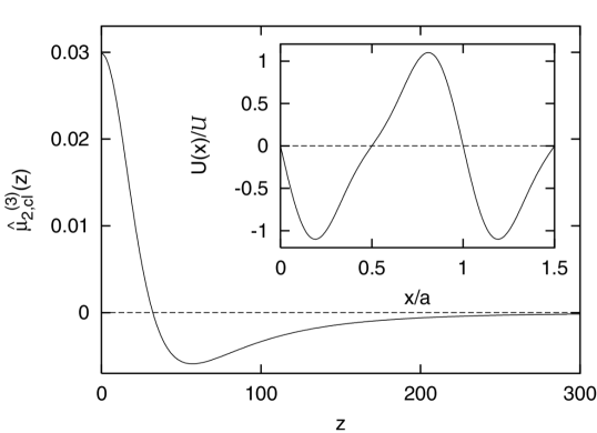
Figure 1: Scaling function ${\hat{\mu}}_{2,\textrm{cl}}^{(3)}(z)$ for the potential (72) shown in the inset.

We explicitly compare our perturbative result for the rectified velocity as a function of temperature – displayed in Fig. 2 – with the exact solution displayed in Fig. 1a of Ref. Bartussek et al., 1994. Thereby, length, energy and time scales are fixed by the choices $a=1$, ${\mathcal{U}}=\frac{1}{2\pi}$, and $\eta=1$. The monochromatic driving force is $F(t)={\mathcal{F}}\sin(\omega t)$ with amplitude ${\mathcal{F}}=0.5$. From the shape of the scaling function it is clear that we find a current reversal with varying temperature for every $\omega>0$ and also a current reversal with varying frequency for every finite $T$. The quantitative agreement is good for $T\gtrsim{\mathcal{U}}$, where the perturbation theory in $U$ is justified.

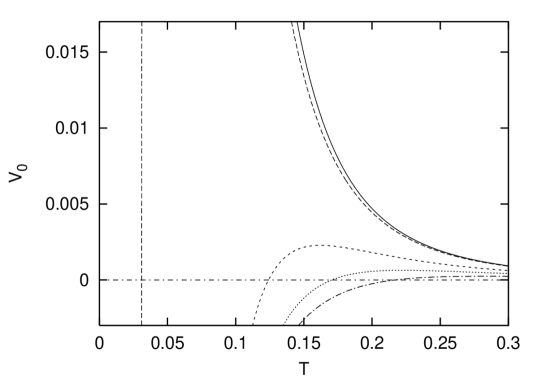
Figure 2: $V_{0}(T)$ for $\omega=0.01$ (bold line), $\omega=1$ (long dashes), $\omega=4$ (short dashes), $\omega=5.5$ (dotted), and $\omega=7$ (dash-dotted) for comparison with Fig. 1a in Ref. Bartussek et al., 1994. The vertical line represents the vicinity of the current reversal for $\omega=1$.

The classical limit is not restricted to single current reversals. It is likely that an arbitrary number of current reversals can be obtained by suitably tailored potential. We have found, for example, that it is sufficient to add one more harmonic to obtain a second current reversal. Specifically, the potential

$$U(x)=-{\mathcal{U}}\left[\sin(2\pi\frac{x}{a})+\frac{1}{4}\sin(4\pi\frac{x}{a})+\frac{1}{4}\sin(6\pi\frac{x}{a})\right]$$ (73)

leads to the scaling function shown in Fig. 3 with two zeroes, i.e., two current reversals.

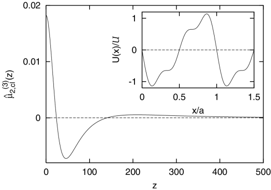
Figure 3: Scaling function ${\hat{\mu}}_{2,\textrm{cl}}^{(3)}(z)$ for the potential (73) shown in the inset.

V.3 Limit $T\to\infty$ for $m>0$

It is interesting to examine the high-temperature limit since there are significant differences between the cases $m=0$ and $m>0$. For $T\to\infty$, the exponential factor in Eq. (60) strongly suppresses $B^{(3)}_{\{q\}}$ and thus $\mu_{2}^{(3)}$. In this limit, we find the asymptotic behavior of the mobility (see appendix D)

$${\hat{\mu}}_{2}^{(3)}(\hat{\hbar},\hat{T},{\hat{\omega}})\to\frac{\hat{\hbar}^{2}\hat{T}^{-17/6}}{1+{\hat{\omega}}^{2}}{\hat{\mu}}_{2,\textrm{hT}}^{(3)},$$ (74a)

or

$$\mu_{2}^{(3)}(-\omega,\omega)=\frac{1}{\eta}\frac{a{\mathcal{U}}^{3}}{(\eta a^{2}\gamma)^{4}}\left(\frac{\eta a^{2}\gamma}{T}\right)^{17/6}\frac{{\hat{\mu}}_{2,\textrm{hT}}^{(3)}}{1+\omega^{2}/\gamma^{2}}$$ (74b)

with

$${\hat{\mu}}_{2,\textrm{hT}}^{(3)} \equiv 2\sqrt{2\pi}\Gamma(\frac{1}{3})\sum_{q_{1}>0,q_{3}>0}\hat{U}^{(3)}_{\{q\}}\hat{q}_{1}^{2}$$ (74c)

$$\times\left(\frac{(\hat{q}_{1}+\hat{q}_{3})^{2}\hat{q}_{3}}{\hat{q}_{1}^{5}}\right)^{1/3}\left(\frac{3^{1/3}\hat{q}_{1}^{2}}{\hat{q}_{1}^{2}+\hat{q}_{3}^{2}}-\frac{1}{6}\right).$$

The constant ${\hat{\mu}}_{2,\textrm{hT}}^{(3)}$ is uniquely determined by the shape of the potential. In the high temperature limit, the rectified current is much stronger for massive particles than for massless cases, since $\mu_{2}^{(3)}\sim T^{-17/6}$ for $m>0$ whereas $\mu_{2}^{(3)}\sim T^{-4}$ for $m=0$, cf. Eq. (71b). This observation is consistent with the mass dependence in Eq. (74), $\mu_{2}^{(3)}\sim m^{7/6}T^{-17/6}$ for $m\to 0$, which signals that in the limit $m\to 0$, $\mu_{2}^{(3)}$ should decay with a higher power of temperature. Thus, inertial terms are crucial at high temperatures even for large friction where the relaxation of the particle in the minima of the potential is overdamped.

V.4 Limit $\omega\to\infty$

For large frequencies, Eq. (59) simplifies to

$${\hat{\mu}}_{2}^{(3)}(\hat{\hbar},\hat{T},{\hat{\omega}})\to\frac{1}{{\hat{\omega}}^{2}(1+{\hat{\omega}}^{2})}{\hat{\mu}}_{2,\textrm{hf}}^{(3)}(\hat{\hbar},\hat{T})$$ (75a)

or

$$\mu_{2}^{(3)}(-\omega,\omega)=\frac{a{\mathcal{U}}^{3}}{\eta(\eta a^{2}\omega)^{2}\hbar^{2}(\gamma^{2}+\omega^{2})}{\hat{\mu}}_{2,\textrm{hf}}^{(3)}(\hat{\hbar},\hat{T})$$ (75b)

with

$${\hat{\mu}}_{2,\textrm{hf}}^{(3)}(\hat{\hbar},\hat{T}) \equiv -\sum_{q_{1}q_{2}q_{3}}\hat{U}^{(3)}_{\{q\}}a^{3}q_{1}\{q_{1}^{2}+q_{1}q_{3}+q_{3}^{2}\}$$ (75c)

$$\times\hbar^{2}\gamma^{2}B^{(3)}_{\{q\}}(0,0).$$

[For the discussion of this limit, $B^{(3)}_{\{q\}}(0,0)\equiv B^{(3)}_{\{q\}}(\omega=0,\omega=0)$.] ${\hat{\mu}}_{2,\textrm{hf}}^{(3)}$ is a function of the potential shape and of to parameters measuring the strength of quantum and thermal fluctuations. In the special case $\hbar=m=0$ we found in Sec. V.2 a momentum dependence $B^{(3)}_{\{q\}}(0,0)\propto q_{2}/q_{1}$ which led to a cancellation in the sum over momenta in expression (75c). Using the fluctuation-dissipation relation (28), one can easily show that $B^{(3)}_{\{q\}}(0,0)$ is independent of $m$ for $\hbar=0$. Thus, this cancellation persists as long as $\hbar=0$, i.e., ${\hat{\mu}}_{2,\textrm{hf}}^{(3)}(0,z)=0$. For $m>0$ this implies a decay $\mu_{2}^{(3)}(-\omega,\omega)\propto\omega^{-6}$. However, such a cancellation can no longer be expected for $\hbar>0$. In this case, one finds again $\mu_{2}^{(3)}(-\omega,\omega)\propto\omega^{-4}$ at large frequencies.

V.5 Limit $\omega\to 0$

A further limit of interest is the adiabatic limit for the quantum particle. This limit was also studied in the pastReimann et al. (1997); Yukawa et al. (1997); Tatara et al. (1998) and has revealed that additional current reversals may arise from the competition of quantum and thermal fluctuations.

For $\omega\to 0$, Eq. (59) reduces to

$${\hat{\mu}}_{2}^{(3)}(\hat{\hbar},\hat{T},0) \equiv -\sum_{q_{1}q_{2}q_{3}}\hat{U}^{(3)}_{\{q\}}\iint_{0}^{\infty}d\hat{t}^{\prime}d\hat{t}^{\prime\prime}$$ (76a)

$$\times\hat{q}_{1}(\hat{q}_{1}\hat{t}^{\prime}-\hat{q}_{3}\hat{t}^{\prime\prime})^{2}\hat{B}^{(3)}_{\{q\}}(\hat{t}^{\prime},\hat{t}^{\prime\prime})$$

with

$$\hat{B}^{(3)}_{\{q\}}({\hat{t}}^{\prime},{\hat{t}}^{\prime\prime})\equiv\hbar^{2}B^{(3)}_{\{q\}}({\hat{t}}^{\prime}/\gamma,{\hat{t}}^{\prime\prime}/\gamma)$$ (76b)

We have calculated ${\hat{\mu}}_{2,\textrm{ad}}^{(3)}$ numerically for $\hat{\hbar}=\frac{1}{\pi}$ [i.e. $\alpha=\eta a^{2}/(2\pi\hbar)=\frac{1}{2}$ corresponding to the delocalized case, cf. Eq. (54)] as a function of temperature (cf. Fig. 4) for the potential (72). The two poles of the double-logarithmic plot in Fig. 4 represent current reversals. At high temperatures, the relation ${\hat{\mu}}_{2}^{(3)}\propto T^{-17/6}$ is recovered (dashed line). At zero temperature, a finite current is generated by quantum fluctuations.

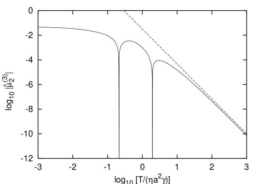
Figure 4: Double logarithmic plot of the rectified velocity [the dimensionless quantity ${\hat{\mu}}_{2,\textrm{ad}}^{(3)}$ given in Eq. (76)] versus temperature in the adiabatic limit for the potential (72) in the underdamped case $\alpha=\frac{1}{2}$ (bold line). The dashed line is a guide to the eye representing the behavior $\propto T^{-17/6}$ of the high-temperature limit.

VI Conclusions

We have developed a perturbative approach for quantum ratchets, which captures current rectification and reversals of the current direction. Our main results are the analytic expression (59) for the leading nonlinear mobility and its evaluation for various limiting cases. In particular, the high-temperature limit for massive particles has revealed the relevance of inertial terms even for strong damping. Since the rectified current decays like $V_{0}\propto T^{-4}$ for massless particles whereas it decays like $V_{0}\propto T^{-17/6}$ for massive particles, inertial effect can lead to a substantial enhancement of ratchet effects. On the other hand, in the high-frequency limit, the quantum nature of the particle is important. While $V_{0}\propto\omega^{-6}$ for massive classical particles, quantum fluctuations also enhance the rectified currant, leading to $V_{0}\propto\omega^{-4}$.

While our perturbative approach is limited to weak potentials and driving forces, it has the advantage that it can be easily generalized to higher dimensions. Therefore, applications for example to asymmetric antidot arraysLorke et al. (1998) become possible. Furthermore, a generalization to random ratchet potentials is obvious. Thereby one could describe the case of asymmetric potential wells with random positions. This generalization can be achieved if one allows for continuous wave vectors $q$ of the potential and simply replaces $U_{q_{1}}U_{q_{2}}U_{q_{3}}$ by its average in the nonlinear mobility (59). An extension of this perturbative approach from single quantum particles to electron gases is under current investigation by the authors.

Appendix A Velocity

In this appendix we show that the average velocity can be calculated from the definition (13). It is this definition in which we deviate from the approach of Fisher and Zwerger.Fisher and Zwerger (1985); Zwerger (1987)

The original definition (3a), in a more explicit form, is based on the average distance the particle travels in a large time interval,

$$V \equiv \frac{X(t_{\textrm{f}})-X(t_{\textrm{i}})}{t_{\textrm{f}}-t_{\textrm{i}}}$$ (77)

in the limit $t_{\textrm{f}}\to\infty$ and $t_{\textrm{i}}\to-\infty$. Thereby the position expectation value (3b) and the time evolution (5a) of the density matrix. On the other hand, the time average of $V(t)$, Eq. (13), can be written as

$$\overline{V(t)} \equiv \frac{{\widetilde{X}}(t_{\textrm{f}})-{\widetilde{X}}(t_{\textrm{i}})}{t_{\textrm{f}}-t_{\textrm{i}}}$$ (78)

with

$${\widetilde{X}}(t) \equiv \int dx\ x{\widetilde{P}}(t,x),$$ (79a)

$${\widetilde{P}}(t,x) \equiv \langle\delta(x-x(t))\rangle.$$ (79b)

A priori, ${\widetilde{P}}(t,x)$, which is an expectation value in an ensemble of paths of length $t_{\textrm{f}}-t_{\textrm{i}}$, is different from $P(x,t)$, Eq. (4), which is an expectation value in an ensemble of paths of length $t-t_{\textrm{i}}$. However, the definitions coincide for $t=t_{\textrm{f}}$ and also for $t=t_{\textrm{i}}$. In the first case the definitions coincide, in the second case because one can integrate out the paths (the integral corresponds to $Z$, Eq. (12), the integral is most easily performed for a diagonal initial density matrix). Thus,

$${{\widetilde{X}}(t_{\textrm{f}})-{\widetilde{X}}(t_{\textrm{i}})}={X(t_{\textrm{f}})-X(t_{\textrm{i}})}$$ (80)

and $V=\overline{V(t)}$. If there is a well defined expectation value $V(t)\equiv\langle\dot{x}(t)\rangle=\frac{d}{dt}{\widetilde{X}}(t)$ for $t_{\textrm{i}}\to-\infty$ and $t_{\textrm{f}}\to\infty$, it must coincide with $\overline{V(t)}$ since boundary effects from times near $t_{\textrm{i}}$ and $t_{\textrm{f}}$ should become negligible in this limit.

Appendix B Calculation of $\mu_{1}^{(2)}$

Here we present intermediate steps of the calculation leading to Eq. (44). In a first step, we need to evaluate

$$\frac{\delta^{2}}{\delta\rho(t)\delta\sigma(t^{\prime})}{\mathcal{Z}} = \Big{\{}iG(t-t^{\prime})+\iint d{\tau_{1}}d{\tau_{2}}[W(t-{\tau_{1}})\rho({\tau_{1}})$$ (81)

$$+ iG(t-{\tau_{1}})\sigma({\tau_{1}})]\rho({\tau_{2}})iG({\tau_{2}}-t^{\prime})\Big{\}}{\mathcal{Z}}$$

where Eqs. (38) have to be inserted for $n=2$. Thereby,

$${\mathcal{Z}}=e^{q_{1}W_{12}q_{2}+q_{1}iG_{12}{s_{2}}q_{2}+q_{2}iG_{21}{s_{1}}q_{1}}\delta_{q_{1}+q_{2},0}$$ (82)

where we abbreviate $W_{kl}\equiv W(t_{k}-t_{l})$ etc. and we used $W(0)=G(0)=0$. Note that in the last exponential, $G_{12}$ or $G_{21}$ vanishes for all $t_{1}$, $t_{2}$ because of causality. Inserting Eq. (81) into Eqs. (36) and (21), only the last of the three terms coming from Eq. (81) survives summation over $s_{j}$ in Eq. (21). One obtains

$$\mu_{1}^{(2)}(t-t^{\prime}) = -i\sum_{q_{1}q_{2}{s_{1}}{s_{2}}}\frac{U_{q_{1}}U_{q_{2}}}{4{s_{1}}{s_{2}}}\iint dt_{1}dt_{2}\dot{G}(t-t_{1}){s_{1}}q_{1}[q_{1}G(t_{1}-t^{\prime})+q_{2}G(t_{2}-t^{\prime})]{\mathcal{Z}}.$$ (83)

In these remaining terms, the summation over ${s_{j}}$ yields

$$\mu_{1}^{(2)}(t-t^{\prime}) = -\sum_{q_{1}q_{2}}U_{q_{1}}U_{q_{2}}\iint dt_{1}dt_{2}\dot{G}(t-t_{1})q_{1}[q_{1}G(t_{1}-t^{\prime})+q_{2}G(t_{2}-t^{\prime})]B_{q_{1}q_{2}}^{(2)}(t_{1}-t_{2}),$$ (84a)

$$B_{q_{1}q_{2}}^{(2)}(t_{1}-t_{2}) \equiv \sum_{{s_{1}}{s_{2}}}\frac{i}{4{s_{1}}{s_{2}}}{s_{1}}{\mathcal{Z}}=\frac{2}{\hbar}\sin(\frac{\hbar}{2}q_{1}^{2}G_{12})\exp(-q_{1}^{2}W_{12})\delta_{q_{1}+q_{2},0}.$$ (84b)

Fourier transforming this expression leads to Eq. (44).

Appendix C Calculation of $\mu_{2}^{(3)}$

Following the same route as for $\mu_{1}^{(2)}$, we first calculate

$$\frac{\delta^{3}}{\delta\rho(t)\delta\sigma(t^{\prime})\delta\sigma(t^{\prime\prime})}{\mathcal{Z}} = \int d\tau\rho(\tau)[iG(t-t^{\prime})iG(\tau-t^{\prime\prime})+iG(t-t^{\prime\prime})iG(\tau-t^{\prime})]{\mathcal{Z}}$$ (85)

$$+\int d\tau[W(t-\tau)\rho(\tau)+iG(t-\tau)\sigma(\tau)]$$

$$\times\int d\tau^{\prime}\rho(\tau^{\prime})iG(\tau^{\prime}-t^{\prime})\int d\tau^{\prime\prime}\rho(\tau^{\prime})iG(\tau^{\prime\prime}-t^{\prime\prime}){\mathcal{Z}}.$$

Eq. (38) leads to

$${\mathcal{Z}}=e^{q_{1}W_{12}q_{2}+q_{1}W_{13}q_{3}+q_{2}W_{23}q_{3}+[q_{2}iG_{21}+q_{3}iG_{31}]q_{1}{s_{1}}+[q_{1}iG_{12}+q_{3}iG_{32}]q_{2}{s_{2}}+[q_{1}iG_{13}+q_{2}iG_{23}]q_{3}{s_{3}}}\delta_{\{q\}}$$ (86)

with $\delta_{\{q\}}\equiv\delta_{q_{1}+q_{2}+q_{3},0}$. Considering the right-hand side of Eq. (85) as a sum of four contributions, the first three disappear after summation over the $s_{j}$. For example, if $t_{1}<t_{2}<t_{3}$, ${\mathcal{Z}}$ is independent of $s_{3}$ and the summation over $s_{3}$ leads to a cancellation. The remaining fourth contribution to Eq. (85) reads explicitly [$\Theta_{23}\equiv\Theta(t_{2}-t_{3})$]

$$\mu_{2}^{(3)}(t-t^{\prime},t-t^{\prime\prime}) = -\sum_{q_{1},q_{2},q_{3},{s_{1}},{s_{2}},{s_{3}}}\frac{U_{q_{1}}}{2i{s_{1}}}\frac{U_{q_{2}}}{2i{s_{2}}}\frac{U_{q_{3}}}{2i{s_{3}}}\iiint dt_{1}dt_{2}dt_{3}\ \Theta_{23}\dot{G}(t-t_{1}){s_{1}}q_{1}$$ (87)

$$\times\{q_{1}G(t_{1}-t^{\prime})q_{1}G(t_{1}-t^{\prime\prime})+q_{2}G(t_{2}-t^{\prime})q_{2}G(t_{2}-t^{\prime\prime})+q_{3}G(t_{3}-t^{\prime})q_{3}G(t_{3}-t^{\prime\prime})$$

$$+q_{1}q_{2}[G(t_{1}-t^{\prime})G(t_{2}-t^{\prime\prime})+G(t_{1}-t^{\prime\prime})G(t_{2}-t^{\prime})]$$

$$+q_{1}q_{3}[G(t_{1}-t^{\prime})G(t_{3}-t^{\prime\prime})+G(t_{1}-t^{\prime\prime})G(t_{3}-t^{\prime})]$$

$$+q_{2}q_{3}[G(t_{2}-t^{\prime})G(t_{3}-t^{\prime\prime})+G(t_{2}-t^{\prime\prime})G(t_{3}-t^{\prime})]\}{\mathcal{Z}}$$

where we used permutation symmetries among indices $j$ which allow us to restrict the time integrals to $t_{2}>t_{3}$. Then, summation over $\{s\}$ leads to

$$B_{q_{1}q_{2}q_{3}}^{(3)}(t_{1}-t_{2},t_{2}-t_{3}) \equiv \Theta_{23}\sum_{{s_{1}}{s_{2}}{s_{3}}}\frac{1}{2{s_{1}}}\frac{1}{2{s_{2}}}\frac{1}{2{s_{3}}}{s_{1}}i^{2}{\mathcal{Z}}$$ (88)

$$= \Theta_{23}\frac{4}{\hbar^{2}}\sin[\frac{\hbar}{2}q_{1}G_{12}q_{2}]\sin[\frac{\hbar}{2}(q_{1}G_{13}q_{3}+q_{2}G_{23}q_{3})]e^{q_{1}W_{12}q_{2}+q_{2}W_{23}q_{3}+q_{1}W_{13}q_{3}}\delta_{\{q\}}.$$ (89)

Note that $B^{(3)}_{\{q\}}\neq 0$ only for $t_{1}>t_{2}>t_{3}$. In terms of $B^{(3)}_{\{q\}}\equiv B^{(3)}_{q_{1}q_{2}q_{3}}$ we obtain

$$\mu_{2}^{(3)}(t-t^{\prime},t-t^{\prime\prime}) = i\sum_{q_{1},q_{2},q_{3}}U_{q_{1}}U_{q_{2}}U_{q_{3}}\iiint dt_{1}dt_{2}dt_{3}\ \dot{G}(t-t_{1})q_{1}$$ (90a)

$$\times\{q_{1}G(t_{1}-t^{\prime})q_{1}G(t_{1}-t^{\prime\prime})+q_{2}G(t_{2}-t^{\prime})q_{2}G(t_{2}-t^{\prime\prime})+q_{3}G(t_{3}-t^{\prime})q_{3}G(t_{3}-t^{\prime\prime})$$

$$+q_{1}q_{2}[G(t_{1}-t^{\prime})G(t_{2}-t^{\prime\prime})+G(t_{1}-t^{\prime\prime})G(t_{2}-t^{\prime})]$$

$$+q_{1}q_{3}[G(t_{1}-t^{\prime})G(t_{3}-t^{\prime\prime})+G(t_{1}-t^{\prime\prime})G(t_{3}-t^{\prime})]$$

$$+q_{2}q_{3}[G(t_{2}-t^{\prime})G(t_{3}-t^{\prime\prime})+G(t_{2}-t^{\prime\prime})G(t_{3}-t^{\prime})]\}B^{(3)}_{\{q\}}(t_{1}-t_{2},t_{2}-t_{3})$$

or, after Fourier transformation,

$$\mu_{2}^{(3)}(\omega^{\prime},\omega^{\prime\prime}) = (\omega^{\prime}+\omega^{\prime\prime})G(\omega^{\prime}+\omega^{\prime\prime})G(\omega^{\prime})G(\omega^{\prime\prime})\sum_{q_{1}q_{2}q_{3}}U_{q_{1}}U_{q_{2}}U_{q_{3}}q_{1}$$ (90b)

$$\times\{q_{1}^{2}B^{(3)}_{\{q\}}(0,0)+q_{2}^{2}B^{(3)}_{\{q\}}(\omega^{\prime}+\omega^{\prime\prime},0)+q_{3}^{2}B^{(3)}_{\{q\}}(\omega^{\prime}+\omega^{\prime\prime},\omega^{\prime}+\omega^{\prime\prime})$$

$$+q_{1}q_{2}[B^{(3)}_{\{q\}}(\omega^{\prime},0)+B^{(3)}_{\{q\}}(\omega^{\prime\prime},0)]+q_{1}q_{3}[B^{(3)}_{\{q\}}(\omega^{\prime},\omega^{\prime})+B^{(3)}_{\{q\}}(\omega^{\prime\prime},\omega^{\prime\prime})]$$

$$+q_{2}q_{3}[B^{(3)}_{\{q\}}(\omega^{\prime}+\omega^{\prime\prime},\omega^{\prime})+B^{(3)}_{\{q\}}(\omega^{\prime}+\omega^{\prime\prime},\omega^{\prime\prime})]\}.$$

Ratchet effects are related to $\omega^{\prime\prime}=-\omega^{\prime}=\omega$, for which Eq. (59) follows after usage of momentum conservation.

Appendix D Details for $T\to\infty$

Although straightforward, the calculation for the high-temperature limit requires some care. For this calculation, it is convenient to rewrite Eq. (59) as

$$\mu_{2}^{(3)}(-\omega,\omega) = -\frac{i}{\eta}\frac{1}{\eta^{2}\omega^{2}+m^{2}\omega^{4}}\sum_{q_{1}q_{2}q_{3}}^{\prime}U_{q_{1}}U_{q_{2}}U_{q_{3}}q_{1}\iint_{0}^{\infty}dt_{12}dt_{23}F^{(3)}_{\{q\}}(\omega,t_{12},t_{23})\exp[-E^{(3)}_{\{q\}}(t_{12},t_{23})]$$ (91)

with $t_{jk}\equiv t_{j}-t_{k}$, $t_{13}=t_{12}+t_{23}$,

$$F^{(3)}_{\{q\}}(\omega,t_{12},t_{23}) \equiv 2\{q_{1}q_{2}[1-\cos(\omega t_{12})]+q_{1}q_{3}[1-\cos(\omega t_{13})]+q_{2}q_{3}[1-\cos(\omega t_{23})]\}$$ (92a)

$$\times\frac{2}{\hbar}\sin[\frac{\hbar}{2}q_{1}G(t_{12})q_{2}]\frac{2}{\hbar}\sin[\frac{\hbar}{2}(q_{1}G(t_{13})q_{3}+q_{2}G(t_{23})q_{3})],$$

and

$$E^{(3)}_{\{q\}}(t_{12},t_{23}) \equiv -[q_{1}W(t_{12})q_{2}+q_{2}W(t_{23})q_{3}+q_{1}W(t_{13})q_{3}]=\frac{1}{2}\langle[q_{1}x(t_{1})+q_{2}x(t_{2})+q_{3}x(t_{3})]^{2}\rangle_{0}\geq 0.$$ (92b)

With increasing $T$, the rectified current shrinks since $E^{(3)}_{\{q\}}$ increases proportional to temperature. The dominant contributions come from small $t_{12}$ and small $t_{23}$. We proceed with an expansion of $E^{(3)}_{\{q\}}$ and $F^{(3)}_{\{q\}}$ to extract the leading orders for large $T$.

In the high-temperature limit, one can neglect the quantum contribution to $W$ and expands for small times (using $q_{2}=-q_{1}-q_{3}$ because of momentum conservation)

$$E^{(3)}_{\{q\}} = \frac{Tm}{\eta^{2}}\bigg{\{}\frac{(q_{1}^{2}+q_{3}^{2})^{2}}{2q_{3}^{2}}{\hat{t}_{-}}^{2}+\frac{1}{3}q_{1}^{2}\frac{q_{1}+q_{3}}{q_{3}}{\hat{t}_{+}}^{3}$$ (93)

$$+O({\hat{t}_{-}}^{3},{\hat{t}_{-}}^{2}{\hat{t}_{+}},{\hat{t}_{-}}{\hat{t}_{+}}^{2},{\hat{t}_{+}}^{4})\bigg{\}}.$$

We introduced dimensionless times ${\hat{t}_{+}}$ and ${\hat{t}_{-}}$ via

$$\gamma t_{12} \equiv {\hat{t}_{+}}-\frac{q_{1}}{q_{3}}{\hat{t}_{-}},$$ (94a)

$$\gamma t_{23} \equiv {\hat{t}_{-}}+\frac{q_{1}}{q_{3}}{\hat{t}_{+}}.$$ (94b)

To extract the asymptotics for $T\to\infty$, one has to distinguish the contributions for $q_{1}/q_{3}>0$ and $q_{1}/q_{3}<0$ (remember that one needs to consider only $q_{1}\neq 0\neq q_{3}$). Because of causality, the time integrals cover only the quadrant with $t_{12}>0$ and $t_{23}>0$ in the $(t_{12},t_{23})$ plane. This quadrant corresponds to ranges

$${\hat{t}_{+}}>0\textrm{ and }-\frac{q_{1}}{q_{3}}{\hat{t}_{+}}<{\hat{t}_{-}}<\frac{q_{3}}{q_{1}}{\hat{t}_{+}} \frac{q_{1}}{q_{3}}>0,$$ for (95a)

$${\hat{t}_{-}}>0\textrm{ and }\frac{q_{1}}{q_{3}}{\hat{t}_{-}}<{\hat{t}_{+}}<-\frac{q_{3}}{q_{1}}{\hat{t}_{-}} \frac{q_{1}}{q_{3}}<0.$$ for (95b)

The integrals are transformed via

$$dt_{12}dt_{23}=\frac{q_{1}^{2}+q_{3}^{2}}{\gamma^{2}q_{3}^{2}}d{\hat{t}_{+}}d{\hat{t}_{-}}.$$ (96)

For $q_{1}/q_{3}<0$, it is sufficient to retain the quadratic term in Eq. (93) since it implies that ${\hat{t}_{-}}\sim T^{-1/2}$. Then also ${\hat{t}_{+}}\sim T^{-1/2}$ according to Eq. (95), i.e., $t_{12}\sim t_{23}\sim T^{-1/2}$. Since $F^{(3)}_{\{q\}}$ is quartic in small times,

$$F^{(3)}_{\{q\}} = \frac{\omega^{2}}{\eta^{2}\gamma^{2}}(q_{1}^{2}+q_{3}^{2})^{3}\frac{q_{1}(q_{1}+q_{3})}{q_{3}^{2}}{\hat{t}_{-}}^{3}(\frac{q_{1}}{q_{3}}{\hat{t}_{-}}-{\hat{t}_{+}})$$ (97)

$$+O(T^{-5/2}),$$

the resulting contributions to $\mu_{2}^{(3)}$ will be of order $T^{-3}$. These terms can be neglected in comparison to terms of order $T^{-17/6}$ which come from $q_{1}/q_{3}>0$.

For $q_{1}/q_{3}>0$ it is not sufficient to retain the quadratic term in Eq. (93) since the integral over ${\hat{t}_{+}}$ would diverge. Thus, one has to include cubic orders in $E^{(3)}_{\{q\}}$ which imply that ${\hat{t}_{+}}\sim T^{-1/3}$. Consequently, the higher order terms not explicitly written in Eq. (93) can be neglected. Since $F^{(3)}_{\{q\}}\sim{\hat{t}_{-}}^{4}\sim T^{-2}$ we now expect $\mu_{2}^{(3)}\sim T^{-17/6}$. The proper expansion of $F^{(3)}_{\{q\}}$ up to order $T^{-2}$ now yields

$$F^{(3)}_{\{q\}} = \frac{\omega^{2}}{\eta^{2}\gamma^{2}}(q_{1}+q_{3})(q_{1}^{2}+q_{3}^{2})^{2}\Big{\{}(q_{1}^{2}+q_{3}^{2})\frac{q_{1}}{q_{3}^{2}}{\hat{t}_{-}}^{3}(\frac{q_{1}}{q_{3}}{\hat{t}_{-}}-{\hat{t}_{+}})$$ (98)

$$- \frac{q_{1}^{2}}{2q_{3}^{2}}(q_{1}+q_{3}){\hat{t}_{-}}^{2}{\hat{t}_{+}}^{3}\Big{\}}+O(T^{-13/6}).$$

Thereby it is sufficient to retain even orders in ${\hat{t}_{-}}$ because the integral over ${\hat{t}_{-}}$ can be extended to all real values [ignoring condition (95)] since the quadratic term in (93) provides a cutoff that dominates over the condition (95) (the errors decay exponentially in $T$). Therefore, the leading order $F^{(3)}_{\{q\}}\sim{\hat{t}_{-}}^{3}{\hat{t}_{+}}\sim T^{-11/6}$ will not result in a contribution to $\mu_{2}^{(3)}$ of order $T^{-8/3}$ since it is odd in ${\hat{t}_{-}}$. Performing the time integrals for the remaining terms,

$$\mu_{2}^{(3)}(-\omega,\omega) = -\frac{i}{\eta^{5}\gamma^{2}}\frac{1}{\gamma^{2}+\omega^{2}}\sum_{q_{1},q_{3};q_{1}/q_{3}>0}U_{q_{1}}U_{-q_{1}-q_{3}}U_{q_{3}}$$ (99)

$$\times \frac{q_{1}^{3}}{q_{3}^{4}}(q_{1}+q_{3})(q_{1}^{2}+q_{3}^{2})^{3}\int_{0}^{\infty}d{\hat{t}_{+}}\int_{-\infty}^{\infty}d{\hat{t}_{-}}$$

$$\times \left(\frac{q_{1}^{2}+q_{3}^{2}}{q_{3}}{\hat{t}_{-}}^{4}-\frac{q_{1}+q_{3}}{2}{\hat{t}_{-}}^{2}{\hat{t}_{+}}^{3}\right)e^{-E^{(3)}_{\{q\}}}$$

yields Eq. (74).

References

- Astumian (1997) R. D. Astumian, Science 276, 917 (1997).
- Bier (1997) M. Bier, Contemp. Phys. 38, 371 (1997).
- (3) P. Reimann, preprint cond-mat/0010237.
- Belinicher and Sturman (1980) V. I. Belinicher and B. I. Sturman, Sov. Phys. Usp. 23, 199 (1980).
- Linke et al. (1998a) H. Linke, W. Sheng, A. Löfgren, H. Q. Xu, P. Omling, and P. E. Lindelof, Europhys. Lett. 44, 341 (1998a).
- Linke et al. (1998b) H. Linke, W. Sheng, A. Löfgren, H. Q. Xu, P. Omling, and P. E. Lindelof, Europhys. Lett. 45, 406 (1998b).
- Lorke et al. (1998) A. Lorke, S. Wimmer, B. Jager, J. P. Kotthaus, W. Wegscheider, and M. Bichler, Physica B 251, 312 (1998).
- Zapata et al. (1996) I. Zapata, R. Bartussek, F. Sols, and P. Hänggi, Phys. Rev. Lett. 77, 2292 (1996).
- Falo et al. (1999) F. Falo, P. J. Martinez, J. J. Mazo, and S. Cilla, Europhys. Lett. 45, 700 (1999).
- Weiss et al. (2000) S. Weiss, D. Koelle, J. Müller, R. Gross, and K. Barthel, Europhys. Lett. 51, 499 (2000).
- Goldobin et al. (2001) E. Goldobin, A. Sterck, and D. Koelle, Phys. Rev. E 63, 031111 (2001).
- (12) C. J. Olson, C. Reichhardt, B. Janko, and F. Nori, preprint cond-mat/0102306.
- Jülicher et al. (1997) F. Jülicher, A. Ajdari, and J. Prost, Rev. Mod. Phys. 69, 1269 (1997).
- Feynman et al. (1963) R. P. Feynman, R. B. Leighton, and M. Sands, The Feynman lectures on physics, vol. 1 (Addison-Wesley, Reading, Massachusetts, 1963).
- not (a) For a historical overview, see e.g. the introduction of Ref. Reimann, .
- Magnasco (1993) M. O. Magnasco, Phys. Rev. Lett. 71, 1477 (1993).
- Bartussek et al. (1994) R. Bartussek, P. Hänggi, and J. G. Kissner, Europhys. Lett. 28, 459 (1994).
- Jung et al. (1996) P. Jung, J. G. Kissner, and P. Hänggi, Phys. Rev. Lett. 76, 3436 (1996).
- Reimann et al. (1997) P. Reimann, M. Grifoni, and P. Hänggi, Phys. Rev. Lett. 79, 10 (1997).
- Yukawa et al. (1997) S. Yukawa, M. Kikuchi, G. Tatara, and H. Matsukawa, J. Phys. Soc. Jap. 66, 2953 (1997).
- Tatara et al. (1998) G. Tatara, M. Kikuchi, S. Yukawa, and H. Matsukawa, J. Phys. Soc. Jap. 67, 1090 (1998).
- Mateos (2000) J. L. Mateos, Phys. Rev. Lett. 84, 258 (2000).
- Caldeira and Leggett (1983) A. O. Caldeira and A. J. Leggett, Ann. Phys. (N.Y.) 149, 374 (1983).
- Fisher and Zwerger (1985) M. P. A. Fisher and W. Zwerger, Phys. Rev. B 32, 6190 (1985).
- Zwerger (1987) W. Zwerger, Phys. Rev. B 35, 4737 (1987).
- Feynman and Vernon (1963) R. P. Feynman and F. L. Vernon, Ann. Phys. (N.Y.) 24, 118 (1963).
- Kleinert (1995) H. Kleinert, Path integrals in quantum mechanics, statistics, and polymer physics (World Scientific, Singapore, 1995).
- not (b) We found it convenient to absorb a factor in the definition of in comparison to Refs. Fisher and Zwerger, 1985 and Kleinert, 1995.
- not (c) We employ the usual convention for Fourier transformation, .
- Ambegaokar and Halperin (1969a) V. Ambegaokar and B. I. Halperin, Phys. Rev. Lett. 22, 1364 (1969a).
- Ambegaokar and Halperin (1969b) V. Ambegaokar and B. I. Halperin, Phys. Rev. Lett. 23, 274 (1969b).
- Ivanchenko and Zil’berman (1969) Y. Ivanchenko and L. A. Zil’berman, Sov. Phys. JETP 28, 1272 (1969).
- Nozières and Iche (1979) P. Nozières and G. Iche, J. de Physique 40, 225 (1979).
- Schmid (1983) A. Schmid, Phys. Rev. Lett. 51, 1506 (1983).
- Reimann (2000) P. Reimann, in Lecture Notes in Physics, edited by J. A. Freund and T. Pöschel (Springer, Berlin, 2000), vol. 557.