Shot Noise at High Temperatures

Abstract

We consider the possibility of measuring non-equilibrium properties of the current correlation functions at high temperatures (and small bias). Through the example of the third cumulant of the current (${\cal{S}}_{3}$) we demonstrate that odd order correlation functions represent non-equilibrium physics even at small external bias and high temperatures. We calculate ${\cal{S}}_{3}=y(eV/T)e^{2}I$ for a quasi-one-dimensional diffusive constriction. We calculate the scaling function $y$ in two regimes: when the scattering processes are purely elastic and when the inelastic electron-electron scattering is strong. In both cases we find that $y$ interpolates between two constants. In the low (high) temperature limit $y$ is strongly (weakly) enhanced (suppressed) by the electron-electron scattering.

I introduction

Since its discovery by Schottky in 1918, noise in electrical circuits has been thoroughly investigated. Numerous studies over the past decade, both experimental [1] and theoretical (see Refs. [2, 3] for reviews), emphasized the quantum and the mesoscopic aspects of noise, addressing quite extensively the issue of non-equilibrium ”shot” noise. Shot noise has been employed for probing fundamental physics of interacting electrons in the FQHE regime [4]. Most of previous work focused on current-current correlations, i.e., fluctuations derived from second order current cumulants[7]

$$\mbox{S}_{2}(x,x^{\prime},\omega)=\frac{1}{2}\int d(t-t^{\prime})e^{-i\omega(t-t^{\prime})}\langle\hat{I}(t,x)\hat{I}(t^{\prime},x^{\prime})+\hat{I}(t^{\prime},x^{\prime})\hat{I}(t,x)\rangle,$$ (1)

where $\hat{I}(t,x)$ denotes the instantaneous current operator integrated trough the entire cross-section (at point $x$); $x$ is the direction of the flow of the d.c. current. Equilibrium noise is governed by the Callen-Welton relation, also known as Fluctuation Dissipation Theorem (FDT). It connects the Ohmic part of the conductance $G(\omega)$ with the equilibrium current noise (${\cal{S}}_{2}=\mbox{S}_{2}-I^{2}$ , $I\equiv\langle\hat{I}\rangle$)

$${\cal{S}}_{2}^{eq}(\omega)=\hbar\omega G(\omega)\coth\left(\frac{\hbar\omega}{2T}\right)\,\,.$$ (2)

Let us consider a two-terminal constriction subject to an applied bias, $eV$, which is equal to the difference between the chemical potentials of the left and the right reservoirs $eV=\mu^{L}-\mu^{R}$. The constriction length $L$ is much larger than an elastic mean free path $l=v_{f}\tau$ ($L\gg l$). The value of the d.c. electron current through the system is given by Ohm’s law, $I=GV$. In the absence of electron-electron collisions the second moment of the current fluctuations can be expressed in terms of the equilibrium correlation function, eq. (2) (cf. Ref. [5, 6])

$${\cal{S}}_{2}(\hbar\omega)\!=\!\frac{1}{6}\bigg{[}4{\cal{S}}^{eq}_{2}(\hbar\omega)\!+{\cal{S}}^{eq}_{2}(\hbar\omega\!+\!eV)+{\cal{S}}^{eq}_{2}(\hbar\omega\!-\!eV)\bigg{]}.$$ (3)

Depending on the ratio between the temperature of the system, $T$, the frequency under discussion, $\omega$, and the applied voltage, $V$, one may distinguish among different regimes. In the limit $(eV\gg\mbox{max}\{kT,\omega\})$ the noise, eq.(3), is essentially non-equilibrium (shot noise), and is proportional to the absolute value of the d.c. electric current. For $eV\ll\mbox{max}\{kT,\omega\}$ ${\cal{S}}_{2}$ is mostly thermal, or Nyquist noise. These observations are not system dependent, but rather follow from general considerations, namely the properties of various operators under time reversal transformation.

Since the current operator changes sign under time reversal transformation, any even-order correlation function of the current fluctuations (e.g. ${\cal{S}}_{2}$) taken at zero frequency is invariant under this operation. Assuming that current correlators are functions of the average current, $I$, it follows that even-order correlation functions depend only on the absolute value of the electric current (and are independent of the direction of the current). In the Ohmic regime this means that even-order current correlation functions (at zero frequency) are even functions of the applied voltage. Evidently, this general observation agrees with the result eq. (3) for the second-order correlation function ${\cal{S}}_{2}$ in the diffusive junction.

By contrast, odd-order current correlation functions change their sign under time reversal transformation. In other words, such correlation functions depend on the direction of the current, and not only on its absolute value. Therefore in the Ohmic regime, odd-order correlation functions of current are odd-order functions of the applied voltage. This condition automatically guarantees that odd-order correlation functions vanish at thermal equilibrium.

The present analysis focuses on the simplest, yet non-trivial, example of manifestly out-of-equilibrium correlator, namely the third order current correlation function $\mbox{S}_{3}$. This is the lowest order correlation function which is dominated by non-equilibrium fluctuations even in the regime where the applied bias is small compared with temperature. There are two situations where the study of shot noise under such conditions is called for. Firstly, when the lowering of the temperature of the electron is not facilitated. Secondly, and more interestingly, when one is interested in exploring the correlations in the system above a certain critical (or a characteristic) temperature. On one hand this requires to keep the temperature relatively high. On the other hand, to study low energy features, one is restricted to low values of the voltage.

In this work we argue and subsequently show that for the third order (and in fact all odd order) current cumulant, out-of-equilibrium fluctuations are not masked by large equilibrium noise: ${\cal{S}}_{3}$ remains linear in voltage (and temperature independent) at high temperatures. The first part of our analysis (SectionII) focuses on the temperature dependence of ${\cal{S}}_{3}$, in the limit where the inelastic length is much larger than the system’s size. We find that ${\cal{S}}_{3}$ is proportional to the the d.c. current at all temperatures, and calculate how the proportionality coefficient interpolates between the two asymptotic values, $1/15$ and $1/3$, for $T\ll eV$ and $T\gg eV$ respectively. In the second part of this paper (Section III) we study the effects of inelastic electron-electron scattering. We specifically consider the limit of $l_{\rm in}/L\ll 1$, where $l_{\rm in}$ is the inelastic electron-electron mean free path and $L$ is the length of the conductor. We find that as compared with the elastic case ${\cal{S}}_{3}$ is weakly suppressed in the high temperature limit (by $\sim 15\%$)but is highly enhanced in the low temperature limit (cf. Table I). Similarly to the elastic case ${\cal{S}}_{3}$ is not masked by thermal fluctuations in the high temperature limit.

Our analysis employs the recently developed non-linear $\sigma$-model–Keldysh technique [8, 9, 10]. This approach has been applied to study non-equilibrium noise in the presence of disorder and electron-electron interactions [10]. The main steps to be followed in the analysis below include finding the saddle point of the effective action (eqs. 21 and 56 for the elastic and the inelastic cases respectively) and expanding in soft modes around them (eqs. 25 and 112). The saddle point (or the approximate one in the inelastic case) are connected with the single-particle distribution function, while the soft modes describe the dynamics of the density fluctuations. Both are significantly modified by strong inelastic scattering.

There are of course other methods that can be employed to study non-equilibrium fluctuations. One appealing candidate would be the Shulman-Kogan [11] version of the Boltzmann-Langevin scheme. This method work successfully when ${\cal{S}}_{2}$ is studied. In Section IV we present a short discussion which shows, arguably in an unexpected way, that the traditional kinetic equation approach breaks down when higher order cumulants are addressed. Section V includes a brief discussion.

II The Elastic Case

As has been shown in Ref.[12], by modeling the measurement procedure as coupling of the system to a “quantum galvanometer”, the emerging mathematical object to be studied is

$$\mbox{S}_{3}(x,t;x^{\prime},t^{\prime};x^{\prime\prime},t^{\prime\prime})=\langle T_{c}\hat{I}_{2}(x,t)\hat{I}_{2}(x^{\prime},t^{\prime})\hat{I}_{2}(x^{\prime\prime},t^{\prime\prime})\rangle\,\,.$$ (4)

Here $x$ is a coordinate measured along a quasi one-dimensional wire ($0\leq x\leq L$) of cross-section ${\cal{A}}$; $T_{c}$ is the time ordering operator along the Keldysh contour and $I_{2}$ is a quantum component of the current. Since the process we consider is stationary, the correlation function depends only on differences of time, $\mbox{S}_{3}(t-t^{\prime};t^{\prime}-t^{\prime\prime})$. In Fourier space it can be represented as

$$\mbox{S}_{3}(\omega_{1},\omega_{2})=\int_{c}d(t-t^{\prime})d(t^{\prime}-t^{\prime\prime})e^{-i\omega_{1}(t-t^{\prime})-i\omega_{2}(t^{\prime}-t^{\prime\prime})}\mbox{S}_{3}(t-t^{\prime},t^{\prime}-t^{\prime\prime})\,\,.$$ (5)

(Here we have assumed that the frequencies $\omega_{1},\omega_{2}$ are small compared with the inverse diffusion time along the wire, such that the current fluctuations are independent of the spatial coordinate). We next evaluate the expression, eq. (4), for a particular system, in the hope that the qualitative properties we are after are not strongly system dependent. In the present section we consider non-interacting electrons in the presence of a short-range, delta correlated and weak disorder potential ($\epsilon_{f}\tau\gg\hbar$, where $\tau$ is the elastic mean free time and $\epsilon_{f}$ is the Fermi energy). To calculate $\mbox{S}_{3}$ we employ the $\sigma$-model formalism, recently put forward for dealing with non-equilibrium diffusive systems (for details see Ref.[10]). As was stressed in our previous work this approach is a generalization of the Boltzmann-Langevin kinetic approach [11]. It is comparable to the latter as long as the kinetic approach is applicable to diffusive systems. A direct employment of the kinetic approach, assuming the random force term to be short-ranged correlated in space, does not give correctly the the higher-than-two cumulants of the current. The reasons for that are discussed below (cf. Section IV).

The Hamiltonian of our system of non-interacting electrons in disordered systems is:

$$H_{0}=\int_{\rm Volume}d{\bf r}\bar{\Psi}({\bf r})\bigg{[}-\frac{\hbar^{2}}{2m}(\nabla-{\bf a})^{2}+U_{\rm dis}\bigg{]}\Psi({\bf r}).$$ (6)

Here $c{\bf a}/e$ is a vector potential. The disorder potential is $\delta$-correlated:

$$\langle U_{\rm dis}({\bf r})~{}U_{\rm dis}({\bf r}^{\prime})\rangle=\frac{1}{2\pi\nu\tau}~{}\delta({\bf r}-{\bf r}^{\prime}),$$ (7)

where $\nu$ is the density of states at the Fermi energy.

Following the procedure outlined in Ref. [10], employing the diffusive approximation and focusing on the out-of-equilibrium system, one can write a generating functional, expressed as a path integral over a bosonic matrix field $Q$

$$Z[{\bf a}]=\int{\cal D}Q\exp(iS[Q,{\bf a}])\,\,.$$ (8)

Here the integration is performed over the manifold

$$\int Q(x,t,t_{1})Q(x,t_{1},t^{\prime})dt_{1}=\delta(t-t^{\prime}),$$ (9)

the effective action is given by

$$iS[Q,{\bf a}]=-\frac{\pi\hbar\nu}{4}\mbox{Tr}\big{\{}D\left(\nabla Q+i[{\bf a}_{\alpha}\gamma^{\alpha},Q]\right)^{2}+4i\hat{\epsilon}Q\big{\}}\,\,,$$ (10)

and

$$\gamma_{1}=\left(\matrix{1&0\cr 0&1\cr}\right),\;\gamma_{2}=\left(\matrix{0&1\cr 1&0\cr}\right)\,.$$ (11)

Tr represents summation over all spatio-temporal and Keldysh components. Here ${\bf a}_{1}$ and ${\bf a}_{2}$ are the Keldysh rotated classical and quantum components of ${\bf a}$. Hereafter we focus our attention on ${\bf a}_{1}$, ${\bf a}_{2}$, the components in the direction along the wire. The third order current correlator may now be expressed as functional differentiation of the generating functional $Z[a]$ with respect to $a_{2}$

$$\!\mbox{S}_{3}(\!t_{1}\!-\!t_{2},t_{2}\!-\!t_{3}\!)\!=\frac{ie^{3}}{8}\frac{\delta^{3}Z[a]}{\delta\!a_{2}(x_{1},t_{1})\delta\!a_{2}(x_{2},t_{2})\delta\!a_{2}(x_{3},t_{3})}.$$ (12)

Performing this functional differentiation one obtains the following result

$$\mbox{S}_{3}(\!t_{1}\!-\!t_{2},t_{2}\!-\!t_{3}\!)\!=\frac{e^{3}{\cal{A}}(\pi\hbar\nu D)^{2}}{8}$$ (13)

$$\bigg{\langle}\frac{1}{2}\hat{\mbox{M}}(x_{1},t_{1})\hat{\mbox{I}}^{D}(x_{2},x_{3},t_{2},t_{3})+$$ (14)

$$(x_{1},t_{1}\leftrightarrow\!x_{3},t_{3})+(x_{1},t_{1}\leftrightarrow\!x_{2},t_{2})+$$ (15)

$$\frac{\pi\hbar\nu D}{8}\hat{\mbox{M}}(x_{1},t_{1})\hat{\mbox{M}}(x_{2},t_{2})\hat{\mbox{M}}(x_{3},t_{3})\bigg{\rangle}\,\,.$$ (16)

Here we have defined

$$\hat{I}^{D}(x,x^{\prime},t,t^{\prime})=\mbox{Tr}^{K}\!\bigg{\{}\!Q_{x,t,t^{\prime}}\gamma_{2}Q_{x^{\prime},t^{\prime},t}\gamma_{2}-\delta_{t,t^{\prime}}\gamma_{1}\bigg{\}}\delta_{x,x^{\prime}},$$ (17)

$$\hat{\mbox{M}}(x,t)=\mbox{Tr}^{K}\!\bigg{\{}\!\int\!dt_{1}\bigg{(}[Q_{x,t,t_{1}};\nabla]~{}Q_{x,t_{1},t}\bigg{)}\gamma_{2}\bigg{\}}.$$ (18)

We employ the notations $Q(x,t,t^{\prime})\equiv Q(x,t,t^{\prime})$; $\mbox{Tr}^{K}$ is the trace taken with respect to the Keldysh indices; $\langle\rangle$ denotes a quantum-mechanical expectation value. The matrix $Q$ can be parameterized as

$$Q=\Lambda\exp\left(W\right)\,\,,$$ (19)

where

$$\Lambda W+W\Lambda=0\,\,,$$ (20)

and $\Lambda$ is the saddle point of the action (10)

$$\Lambda(x,\epsilon)=\left(\matrix{1&2F(x,\epsilon)\cr 0&-1\cr}\right)\,\,.$$ (21)

The function $F$ is related to the single particle distribution function $f$ through

$$F(x,\epsilon)=1-2f(x,\epsilon)\,\,.$$ (22)

The matrix $W_{x,\epsilon,\epsilon^{\prime}}$, in turn, is parameterized as follows:

$$W_{x,\epsilon,\epsilon^{\prime}}\!=\!\left(\matrix{F_{x,\epsilon}\bar{w}_{x,\epsilon,\epsilon^{\prime}}&-w_{x,\epsilon,\epsilon^{\prime}}+F_{x,\epsilon}\bar{w}_{x,\epsilon,\epsilon^{\prime}}F_{x,\epsilon^{\prime}}\cr-\bar{w}_{x,\epsilon,\epsilon^{\prime}}&-\bar{w}_{x,\epsilon,\epsilon^{\prime}}F_{x,\epsilon^{\prime}}\cr}\right).$$ (23)

It is convenient to introduce the diffusion propagator

$$(-i\omega+D\nabla^{2})\mbox{D}(x,x^{\prime}\omega)=\frac{1}{\pi\hbar\nu}\delta(x-x^{\prime})\,\,.$$ (24)

The absence of diffusive motion in clean metallic leads implies that the diffusion propagator must vanish at the end points of the constriction. In addition, there is no current flowing in the transversal direction (hard wall boundary conditions). It follows that the component of the gradient of the diffusion propagator in that direction (calculated at the hard wall edges) must vanish as well. The correlation functions of the fields $w,\bar{w}$ are then given by:

$$\langle w(x,\epsilon_{1},\epsilon_{2})\bar{w}(x^{\prime},\epsilon_{3},\epsilon_{4})\rangle=2(2\pi)^{2}\delta(\epsilon_{1}-\epsilon_{4})\delta(\epsilon_{2}-\epsilon_{3})\mbox{D}(x,x^{\prime},\epsilon_{1}-\epsilon_{2})\,,$$ (25)

$$\langle w(x,\epsilon_{1},\epsilon_{2})w(x^{\prime},\epsilon_{3},\epsilon_{4})\rangle=-g(2\pi)^{3}\delta(\epsilon_{1}-\epsilon_{4})\delta(\epsilon_{2}-\epsilon_{3})\int dx_{1}\mbox{D}_{\epsilon_{1}-\epsilon_{2},x,x_{1}}\nabla F_{\epsilon_{2},x_{1}}\nabla F_{\epsilon_{1},x_{1}}\mbox{D}_{\epsilon_{2}-\epsilon_{1},x_{1},x^{\prime}}\,\,,$$ (26)

$$\langle\bar{w}(x,\epsilon_{1},\epsilon_{2})\bar{w}(x^{\prime},\epsilon_{3},\epsilon_{4})\rangle=0\,\,.$$ (27)

It is the the third cumulant (the reduced correlation function) of the current, $S_{3}$, that is of interest to us

$${\cal{S}}_{3}=\mbox{S}_{3}-3I\mbox{S}_{2}+2I^{3}\,\,.$$ (28)

To evaluate $\mbox{S}_{3}$ one follows steps similar to those that led to the derivation of $\mbox{S}_{2}$, see Ref. [10]. If all relevant energy scales in the problem are smaller than the transversal Thouless energy ($E_{Th}=D/L_{T}^{2}$, where $L_{T}$ is a width of a wire), the wire is effectively quasi-one dimensional. In that case only the lowest transversal mode of the diffusive propagator can be taken into account, which yields

$$\mbox{D}(x_{1},x_{2})=\frac{1}{2\pi g}\bigg{[}|x_{1}-x_{2}|-x_{1}-x_{2}+\frac{2x_{1}x_{2}}{L}\bigg{]}\,\,.$$ (29)

Here $g=\hbar\nu D$. The electron distribution function in this system is equal to

$$F(x,\epsilon)=\frac{x}{L}F_{eq}\left(\epsilon-\frac{eV}{2}\right)+\left(1-\frac{x}{L}\right)F_{eq}\left(\epsilon+\frac{eV}{2}\right)\,\,.$$ (30)

The quantities $F$ and D determine the correlation functions, eq. (25). We can now begin to evaluate $\mbox{S}_{3}$, (c.f. eq. (13)), performing a perturbative expansion in the fluctuations around the saddle point solution, eq. (21). After some algebra we find that in the zero frequency limit the third order cumulant is given by

$${\cal{S}}_{3}(\omega_{1}=0,\omega_{2}=0)=\frac{3e^{3}{\cal{A}}\pi g^{2}}{\hbar L^{3}}\int_{0}^{L}dx_{1}dx_{2}$$ (31)

$$\int_{-\infty}^{\infty}d\epsilon F(\epsilon,x_{1})\mbox{D}[0,x_{1},x_{2}]\nabla\left(F^{2}(\epsilon,x_{2})\right)\,\,.$$ (32)

Integrating over energies and coordinates we obtain

$${\cal{S}}_{3}(\omega_{1}=0,\omega_{2}=0)=e^{2}Iy(p)\,\,,$$ (33)

$$y(p)=\frac{6(-1+e^{4p})+(1-26e^{2p}+e^{4p})p}{15p(-1+e^{2p})^{2}}\,\,,$$ (34)

where $p=eV/2T$. The function $y$ is depicted in Fig.1, where it is plotted on a logarithmic scale.

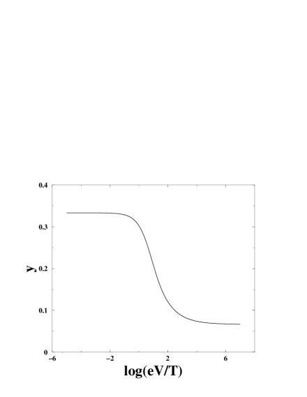
FIG. 1.: The scaling function $y$ plotted on a logarithmic scale, cf. eq. (33)

Let us now discuss the main features of the function $S_{3}$. In agreement with symmetry requirements ${\cal{S}}_{3}$ is an odd function of the voltage (the even correlator ${\cal{S}}_{2}$ is proportional to the absolute value of voltage), and vanishes at equilibrium. The zero temperature result (high voltage limit) has already been obtained by means of the scattering states approach for single-channel systems [13], and later generalized by means of Random Matrix Theory (RMT) to multi-channel systems (chaotic and diffusive) [14]. In our derivation we do not assume the applicability of RMT. Our result covers the whole temperature range. We see that at low temperatures the third order cumulant is linear in the voltage

$${\cal{S}}_{3}=\frac{e^{2}}{15}I\,\,.$$ (35)

At high temperatures the electrons in the reservoirs are not anymore in the ground state, so the correlations are partially washed out by thermal fluctuations. One may then expand $y(p)$, eq. (33), in a series of $eV/2T$. The leading term in this high temperature expansion is linear in the voltage

$${\cal{S}}_{3}=\frac{e^{2}}{3}I\,\,.$$ (36)

Note that although thermal fluctuations enhance the noise (compared with the zero temperature limit), eqs.(35) and (36) differ by only a numerical coefficient. For the symmetry reasons alluded to in the introduction (the vanishing of ${\cal{S}}_{3},\,\,{\cal{S}}_{5}$, etc. at equilibrium), it is tempting to conjecture that all odd order current cumulants interpolate between two constant values as the ratio $eV/kT$ is varied. The experimental study of these cumulants provides one with a direct probe of non-equilibrium behavior, not masked by equilibrium thermal fluctuations.

III Inelastic Case

In our analysis so far we have completely ignored inelastic collisions among the electrons. This procedure is well justified provided that the inelastic length greatly exceeds the system’s size. However, if this is not the case, different analysis is called for. To understand why inelastic collisions do matter for current fluctuations, we would like to recall the analysis of ${\cal{S}}_{2}$ for a similar problem. The latter function is fully determined by the effective electron temperature. Collisions among electrons, which are subject to an external bias, increase the temperature of those electrons. This, in turn, leads to the enhancement of ${\cal{S}}_{2}$, cf. Refs. [15, 16]. In the limit of short inelastic length

$$l_{\rm in}\ll L\,\,,$$ (37)

the zero frequency and zero temperature noise is

$${\cal{S}}_{2}(0)=\frac{\sqrt{3}}{4}eI\,\,.$$ (38)

By comparing with the $\omega,T=0$ limit of eq. (3) we see that inelastic collisions enhance the current fluctuations. In the present section we consider the effect of inelastic electron collisions on ${\cal{S}}_{3}$.

In the present analysis we assume that the electron-phonon collision length is large, $l_{\rm e-ph}\gg L$, hence electron-phonon scattering may be neglected. The Hamiltonian we are concerned with is

$$H=H_{0}+H_{\rm int}.$$ (39)

The Coulomb interaction among the electrons is described by

$$H_{\rm int}=\frac{1}{2}\int d{\bf r}d{\bf r^{\prime}}\bar{\Psi}({\bf r})\bar{\Psi}({\bf r}^{\prime})V_{0}({\bf r}-{\bf r}^{\prime})\Psi({\bf r})\Psi({\bf r}^{\prime})\,\,,$$ (40)

where

$$V_{0}({\bf r}-{\bf r}^{\prime})=\frac{e^{2}}{|{\bf r}-{\bf r}^{\prime}|}\,\,.$$ (41)

We need to deal with the effect of electron-electron interactions in the presence of disorder and away from equilibrium. Following Ref. [8] one may introduce an auxiliary bosonic field

$$\Phi=\left(\begin{array}[]{l}\phi_{1}\\ \phi_{2}\end{array}\right),$$ (44)

which decouples the interaction in the particle-hole channel. Now the partition function (eq. (8)) is a functional integral over both the bosonic fields $Q$ and $\phi$  ,

$$\langle Z\rangle=\int_{Q^{2}=1}{\cal D}Q{\cal D}\phi\exp(iS_{total})\,\,.$$ (45)

The action is

$$iS_{total}=iS[\Phi]+iS[\Phi,Q]\,,$$ (47)

$$iS[\Phi]=i\mbox{Tr}\{\Phi^{T}V^{-1}_{0}\gamma^{2}\Phi\}\,,$$ (48)

$$iS[\Phi,Q]=-\frac{\pi\nu}{4\tau}\mbox{Tr}\{Q^{2}\}\!+\mbox{Tr}\ln\Big{[}\hat{G}_{0}^{-1}\!+\frac{iQ}{2\tau}+\phi_{\alpha}\gamma^{\alpha}\Big{]}.$$ (49)

It is convenient to perform a “gauge transformation” [8] to a new field $\tilde{Q}$

$$Q_{t,t^{\prime}}(x)=\exp\left(ik_{\alpha}(x,t)\gamma^{\alpha}\right)\tilde{Q}_{t,t^{\prime}}(x)\exp\left(-ik_{\alpha}(x,t^{\prime})\gamma^{\alpha}\right)\,.$$ (50)

Introducing the long derivative

$${\bf\partial}_{x}\tilde{Q}\equiv\nabla\tilde{Q}+i[\nabla k_{\alpha}\gamma^{\alpha},\tilde{Q}]\,,$$ (51)

one may write the gradient expansion of eq. (49) as

$$iS[\tilde{Q},\Phi]=i\nu\mbox{Tr}\{(\Phi-i\omega K)^{T}\gamma_{2}(\Phi+i\omega K)\}-$$ (52)

$$\frac{\pi\nu}{4}\left[D\mbox{Tr}\{{\bf\partial}_{x}\tilde{Q}\}^{2}+4i\mbox{Tr}\{(\epsilon+(\phi_{\alpha}+i\omega k_{\alpha})\gamma^{\alpha})\tilde{Q}\}\right]\,\,.$$ (53)

At this point the vector $K^{T}=(k_{1},k_{2})$ that determines the transformation (50) is arbitrary. The saddle point equation for $Q$ of the action (52) is given by the following equation

$$D\partial_{x}(\tilde{Q}\partial_{x}\tilde{Q})+i[(\epsilon+(\phi_{\alpha}+i\omega k_{\alpha})\gamma^{\alpha}),\tilde{Q}]=0\,.$$ (54)

Let us now choose the parameterization

$$\tilde{Q}=\tilde{\Lambda}\exp(\tilde{W}),$$ (55)

where $\tilde{W}$ represents fluctuation around the saddle-point

$$\tilde{\Lambda}(x,\epsilon)=\left(\matrix{1&2\tilde{F}[\phi](x,\epsilon)\cr 0&-1\cr}\right)\,\,.$$ (56)

Eq. (56) implies that the solution of the saddle point, equation (54), determines $\tilde{F}$ as a functional of $\phi$. We do not know, though, how to solve it. Instead we average over $\phi$ on the level of eq.(54). The solution of this averaged equation, denoted by $\bar{F}$, is determined by:

$$D\nabla^{2}\bar{F}(\epsilon)=I^{ee}\{F\}\,,$$ (57)

where the r.h.s. is given by

$$I^{ee}\{\bar{F}\}=D\int\frac{d\omega}{\pi}\big{[}\langle\nabla k^{1}(\omega)\nabla\!k^{1}(-\omega)\rangle\big{(}\bar{F}(\epsilon)-\bar{F}(\epsilon-\omega)\big{)}+$$ (58)

$$\!(\langle\nabla\!k^{1}(\omega)\nabla\!k^{2}(-\omega)\rangle\!-\!\langle\nabla\!k^{2}(\omega)\nabla\!k^{1}(-\omega)\!\rangle)\big{(}\bar{F}(\epsilon)\bar{F}(\epsilon\!-\omega)\!-\!1\big{)}\big{]}.$$ (59)

We stress that our averaging procedure is not related to the genuine interacting saddle point. We will be expanding about another point ($\bar{\Lambda}$) at which the fields $\tilde{W}$ and $\phi,(\nabla k)$ are nearly decoupled; $\tilde{W}$ is parameterized as in eq.(23). Taking variation of the action with respect to $w$, $\bar{w}$, we obtain the following gauge, determining $k[\phi]$:

$$D\nabla^{2}k_{2}-\phi_{2}-i\omega k_{2}=0$$ (60)

$$D\nabla^{2}k_{1}+\phi_{1}+i\omega k_{1}=2\mbox{B}[\omega,x]\nabla^{2}k_{2}\,,$$ (61)

where

$$\mbox{B}[\omega,x]=\frac{1}{2\omega}\int d\epsilon[1-\bar{F}(\epsilon,x)\bar{F}(\epsilon-\omega,x)]\,.$$ (62)

Though we have failed to find the true saddle point the linear part of the action expanded around ($\bar{\Lambda}$) is zero. It is remarkable to notice that under conditions (60) eq.(57) becomes a quantum kinetic equation [17] with the collision integral being $I^{ee}\{F\}$. The above procedure consists of an expansion of the action, eq.(52), around its saddle point. The expansion presumes slow fluctuations in space and time (though the results obtained, expressing ${\cal{S}}_{3}$ in terms of the distribution function and the effective propagator, eq.(110), may be valid under less restrictive conditions). In Fourier space (with respect to the spatial coordinate and the sum–rather than the difference– of the time coordinates) this implies $ql\ll 1$ and $\omega\tau\ll 1$. Hence this procedure implies that the collision integral, $I^{ee}$, appearing in the quantum kinetic equation, eq.(57), accounts only for electron-electron collisions with small momentum transfer. We therefore need to ascertain that these are indeed the small momentum transfer processes which make the dominant contribution to the electron-electron collision rate. To estimate the relative importance of the small and large momentum processes we compare their respective contributions to the energy relaxation time, $\tau_{ee}$. Electron-electron scattering with small momentum transfer leads to result [17, 18]:

$$1/\tau_{ee}=\frac{\epsilon^{d/2}}{\hbar\nu_{d}D^{d/2}}\,\,\,\,ql\ll 1\,\,,$$ (63)

while the contribution coming from large momentum transfer is

$$1/\tau_{ee}=\frac{\pi^{2}}{64}\frac{\epsilon^{2}}{\mu}\frac{\kappa}{p_{F}}\,\,\,\,ql\gg 1\,\,.$$ (64)

As is now clearly seen, for low enough energies

$$\epsilon\ll\left(\frac{64\mu p_{F}}{\pi^{2}\kappa\hbar\nu_{d}D^{d/2}}\right)^{\frac{2}{4-d}}\,\,,$$ (65)

the contribution to the inelastic mean free time coming from scattering with small momentum transfer is dominant; ignoring it would result in seriously overestimating $\tau^{ee}$ time (and correspondingly the mean free path $l_{\rm ee}$).

Coming back to our calculations we note that the correlation function of current fluctuations is a gauged invariant quantity (does not depend on the position of the Fermi level). This means that momenta $q\leq\sqrt{\omega/D}$ do not contribute to such a quantity [19]. In this case the Coulomb propagator is universal, i.e. does not depend on the electron charge. The fact that we address gauge invariant quantities allows us to represent the generating functional $Z$ in terms of the fields $Q$ and $\nabla k$ (rather than $Q$ and $\phi$), as in Ref [8].

$$\langle Z\rangle\!=\!\int\!\!{\cal D}\nabla K\,\exp\left(-i\nu D\mbox{Tr}\{\nabla K^{T}{\cal D}^{-1}\nabla K\}\right)\int{\cal D}\tilde{Q}\,\exp\left(\sum\limits_{l=0}^{2}iS_{l}[\tilde{Q},\nabla K]\right)\,.$$ (66)

Here we define

$${\cal D}^{-1}=\left(\begin{array}[]{cc}0&-D\nabla^{2}_{x}+i\omega\delta_{x,x^{\prime}}\\ -D\nabla^{2}_{x}-i\omega\delta_{x,x^{\prime}}&-2i\omega\delta_{x,x^{\prime}}B_{\omega}(x)\end{array}\right)\,\,,$$ (67)

where the expansion $S=S^{0}+S^{1}+S^{2}$, is in powers of $\nabla K$; the $l-th$ power ($l=0,1,2$) is given by

$$iS^{0}[\tilde{Q}]=-\frac{\pi\nu}{4}\left[D\mbox{Tr}\{\nabla\tilde{Q}\}^{2}+4i\,\mbox{Tr}\{\epsilon\tilde{Q}\}\right]\,,$$ (69)

$$iS^{1}[\tilde{Q},\nabla K]=-i\pi\nu\left[D\mbox{Tr}\{\nabla k_{\alpha}\gamma^{\alpha}\tilde{Q}\nabla\tilde{Q}\}+\mbox{Tr}\{(\phi_{\alpha}+i\omega k_{\alpha})\gamma^{\alpha}\tilde{Q}\}\right]\,,$$ (70)

$$iS^{2}[\tilde{Q},\nabla K]=\frac{\pi\nu D}{2}\left[\mbox{Tr}\{\nabla k_{\alpha}\gamma^{\alpha}\tilde{Q}\nabla k_{\beta}\gamma^{\beta}\tilde{Q}\}-\mbox{Tr}\{\nabla k_{\alpha}\gamma^{\alpha}\tilde{\Lambda}\nabla k_{\beta}\gamma^{\beta}\tilde{\Lambda}\}\right]\,.$$ (71)

From eq.(66) we obtain the gauge field correlation function

$$\langle\nabla k_{\alpha}(x,\omega)\nabla k_{\beta}(x^{\prime},-\omega)\rangle=\frac{i}{D}Y_{\alpha,\beta}(\omega,x,x^{\prime}),$$ (72)

where

$$Y(\omega,x,x^{\prime})=\left[\begin{array}[]{cc}-2i\pi\nu\omega\int dx_{1}\mbox{D}[-\omega,x,x_{1}]\mbox{B}[\omega,x_{1}]\mbox{D}[\omega,x_{1},x^{\prime}]&\mbox{D}[-\omega,x,x^{\prime}]\\ \mbox{D}[\omega,x,x^{\prime}]&0\end{array}\right],$$ (73)

Using eqs.(72,73) we rewrite eq.(58) for the quasi-one-dimensional wire as:

$$D\nabla^{2}\bar{F}(\epsilon)=I^{ee}\{\epsilon,x\}\,,{\rm where}$$ (74)

$$I^{ee}(\epsilon,x)=\frac{i\pi}{2}\int d\omega\big{[}-2i\omega\pi\nu D[x,x_{1},-\omega]B[\omega,x_{1}]\mbox{D}[x_{1},x,\omega]\big{(}\bar{F}(\epsilon)-\bar{F}(\epsilon-\omega)\big{)}+$$ (75)

$$(\mbox{D}[x,x,\omega]-\mbox{D}[x,x,-\omega])(1-\bar{F}(\epsilon)\bar{F}(\epsilon+\omega))\big{]}.$$ (76)

The total number of particles and the total energy of the electrons are both preserved during electron-electron and elastic electron-impurity scattering. The collision integral, eq.(75), satisfies then

$$\int_{-\infty}^{\infty}I^{ee}(\epsilon,x)d\epsilon=0,$$ (77)

$$\int_{-\infty}^{\infty}\epsilon I^{ee}(\epsilon,x)d\epsilon=0.$$ (78)

We now consider the limit $l_{\rm ee}\ll L$. The solution of eq.(57) assumes then the form of a quasi-equilibrium single-particle distribution function

$$\bar{F}(\epsilon,x)=\tanh\left({\frac{\epsilon-e\phi(x)+\bar{\mu}}{2T(x)}}\right).$$ (79)

Here $\epsilon$ is the total energy of the electron, and $e\phi$ is the local electro-chemical potential, i.e. the sum of the local chemical potential $\mu$ and the electrostatic potential $u$ ($e\phi(x)=\mu(x)+eu(x)$); $\bar{\mu}$ is the value of the electro-chemical potential before the bias has been applied and $T(x)$ is the effective local temperature of the electron gas.

Since the size of a constriction is much longer than Debye screening length $\lambda^{-1}_{D}=\sqrt{4\pi e^{2}\nu}$ we may use a quasi-neutrality approximation, in this case to assume that a value of chemical potential $\mu$ is constant in the constriction. It still remains to find the effective electronic temperature, $T(x)$, and the electrostatic potential $u(x)$.

In order to find the electrostatic potential that enters eq.(79) we employ eq. (77). To facilitate our calculations we further assume that conductance band is symmetric about the Fermi energy and that the spectral density of single-electron energy levels is constant. Integration over the energy, eq.(77) yields

$$\partial_{x}^{2}\int\bar{F}(\epsilon)d\epsilon=0$$ (80)

$${\partial_{x}}^{2}u=0.$$ (81)

Solving eq.(81) with the requirement that the electro-chemical potential at the edges of the sample differs by $V$, we find that the electro-chemical potential along the constriction $(0\leq x\leq L)$ is given by

$$e\phi(x)=eV\left(\frac{x}{L}-\frac{1}{2}\right)+\bar{\mu}.$$ (82)

We use the energy conservation property of the collision integral, eq. (78). Multiplying eq. (74) by energy and integrating over it

$$\partial_{x}^{2}\int\epsilon\bar{F}(\epsilon)d\epsilon=0\,\,,$$ (83)

we obtain an equation for the electron temperature:

$$\partial_{x}^{2}\bigg{(}\frac{\pi^{2}}{6}(kT(x))^{2}+\frac{1}{2}(eu(x))^{2}\bigg{)}=0.$$ (84)

The boundary condition of eq.(84) is determined by the temperature of the electrons in the reservoirs. Combining eqs.(83) and (82) we find the electron temperature in two opposite limits:

$$T(x)=\left\{\begin{array}[]{l}\frac{\sqrt{3}eV}{\pi L}\sqrt{x(L-x)}\,\,\,\,\,\,eV\gg T\,\,,\\ \,\,\,\,\,T\hskip 65.44142pteV\ll T\,\,.\end{array}\right.$$ (87)

Eqs.  ((79) , (82)  and (87) determine the function $\bar{F}$ uniquely. We now replace the right-corner element of the matrix $\tilde{\Lambda}$ (i.e. $\tilde{F}[\phi]$, cf. eq.(56)) by its average value $\bar{F}$.

To calculate ${\cal{S}}_{3}$ under conditions of strong electron-electron scattering (eq. (37)) one needs to replace the operators $\hat{\mbox{I}}^{D}$ and $\hat{\mbox{M}}$ in eq.  (13) by their gauged values

$$\mbox{S}_{3}(t_{1}-t_{2},t_{2}-t_{3})=\frac{e^{3}(\pi\hbar\nu D)^{2}}{8}$$ (88)

$$\bigg{\langle}\frac{1}{2}\hat{\tilde{\mbox{M}}}(x_{1},t_{1})\hat{\tilde{\mbox{I}}}^{D}(x_{2},x_{3},t_{2},t_{3})+$$ (89)

$$(x_{1},t_{1}\leftrightarrow\!x_{3},t_{3})+(x_{1},t_{1}\leftrightarrow\!x_{2},t_{2})+$$ (90)

$$\frac{\pi\hbar\nu D}{8}\hat{\tilde{\mbox{M}}}(x_{1},t_{1})\hat{\tilde{\mbox{M}}}(x_{2},t_{2})\hat{\tilde{\mbox{M}}}(x_{3},t_{3})\bigg{\rangle}_{\nabla k,\tilde{Q}}\,\,,$$ (91)

where the averaging is taken over the entire action $S$ and the Gaussian weight function for $\nabla K$, as in eq. (45). Here we define (cf. eqs.(17), (18) with eqs. (92),(93))

$$\hat{\tilde{\mbox{I}}}^{D}(x,x^{\prime},t,t^{\prime})=\mbox{Tr}\!\bigg{\{}\!\tilde{Q}_{x,t,t^{\prime}}\gamma_{2}\tilde{Q}_{x^{\prime},t^{\prime},t}\gamma_{2}-\delta_{t,t^{\prime}}\gamma_{1}\bigg{\}}\delta_{x,x^{\prime}}\,\,,$$ (92)

$$\hat{\tilde{\mbox{M}}}(x,t)=\mbox{Tr}\!\bigg{\{}\!\int\!dt_{1}\bigg{(}[\tilde{Q}_{x,t,t_{1}};\partial_{x}]~{}\tilde{Q}_{x,t_{1},t}\bigg{)}\gamma_{2}\bigg{\}}\,\,,$$ (93)

where the “long derivative”, $\partial_{x}$, is presented in eq.(51). In order to actually perform the functional integration over the matrix field $\tilde{Q}$ we use the parameterization of eq. (55). The operators $\hat{\tilde{\mbox{I}}}^{D},\hat{\tilde{\mbox{M}}}$ may be expanded over $w,\bar{w}$ and $\nabla k$ :

$$\hat{\tilde{\mbox{M}}}=\tilde{\mbox{M}}^{0}_{0}+\tilde{\mbox{M}}^{0}_{1}+\dots+\tilde{\mbox{M}}^{1}_{0}+\tilde{\mbox{M}}^{1}_{1}+\dots$$ (94)

$$\hat{\tilde{\mbox{I}}}^{D}=\tilde{\mbox{I}}_{0}+\tilde{\mbox{I}}_{1}+\dots$$ (95)

Here the upper index refers to the power of the $\nabla k$ fields; the lower refers to the power of $w,\bar{w}$ fields in the expansion. We need to find the Gaussian fluctuations around the saddle point of the action (67). Though we did not find the exact saddle point, the expansion of $Q$ around $\bar{\Lambda}$ works satisfactorily. The coupling between the fields $\nabla k$ and $W$ which appears already in the Gaussian (quadratic) part is small, since it is proportional to the gradient of the distribution function:

$$\!iS^{1}_{1}\!=\!-2i\pi\!g\mbox{Tr}\bigg{\{}\!\bar{w}_{x,\epsilon,\epsilon^{\prime}}[\nabla k_{1x,\epsilon^{\prime}-\epsilon}\nabla\bar{F}_{x,\epsilon}-\nabla\bar{F}_{x,\epsilon^{\prime}}\nabla\!k_{1x,\epsilon^{\prime}-\epsilon}\!+$$ (96)

$$\nabla\bar{F}_{x,\epsilon^{\prime}}\nabla\!k_{2x,\epsilon^{\prime}\epsilon}\bar{F}_{x,\epsilon}+\bar{F}_{x,\epsilon^{\prime}}\nabla\!k_{2x,\epsilon^{\prime}-\epsilon}\nabla\bar{F}_{x,\epsilon}]\bigg{\}}.$$ (97)

Considered as a small perturbation, $iS_{1}^{1}$ does not affect the results.

The more dramatic effect on the correlation function arises from the non-Gaussian part of the action, eqs. (70,71) (by this we mean non-Gaussian terms in either $w,\bar{w}$ or $\nabla K$). After integrating over the interaction an additional contribution to the Gaussian part (proportional to $w\bar{w}$) of the action arises. To find the effective action $iS^{\rm eff}[W]$ we average over the interaction along the following lines:

$$\bigg{\langle}\exp\bigg{\{}iS^{1}+iS^{2}\bigg{\}}\bigg{\rangle}_{\!\!\!\nabla\!k}=$$ (98)

$$\bigg{\langle}\exp\bigg{\{}\bigg{\langle}iS^{1}+iS^{2}\rangle+iS^{1}+iS^{2}-\bigg{\langle}iS^{1}+iS^{2}\bigg{\rangle}\bigg{\}}\bigg{\rangle}_{\!\!\!\nabla\!k}\simeq$$ (99)

$$\!\exp\bigg{\{}\!\bigg{\langle}\!iS^{1}+iS^{2}\bigg{\rangle}_{\!\!\!\nabla\!k}\bigg{\}}\bullet$$ (100)

$$\bigg{[}1\!+\!iS^{1}+iS^{2}\!-\!\bigg{\langle}\!iS^{1}\!+\!iS^{2}\bigg{\rangle}_{\!\!\!\nabla\!k}\!\!\!+\!\frac{1}{2}\!\bigg{(}\!iS^{1}\!+\!iS^{2}\!-\!\bigg{\langle}\!iS^{1}\!+\!iS^{2}\!\bigg{\rangle}_{\!\!\!\nabla\!k}\!\!\bigg{)}^{2}\!\bigg{]}$$ (101)

$$\simeq\!\!\exp\bigg{\{}\bigg{\langle}\!iS^{1}+iS^{2}\!\bigg{\rangle}_{\!\!\!\nabla\!k}\!\!\!\!+\!\!\!\frac{1}{2}\!\bigg{\langle}\!\bigg{(}iS^{1}+iS^{2}\bigg{)}^{2}\bigg{\rangle}_{\!\!\!\nabla\!k}\!\!\!\!\!-\!\!\frac{1}{2}\!\bigg{\langle}\!iS^{1}\!+\!iS^{2}\bigg{\rangle}_{\!\!\!\nabla\!k}^{2}\!\!\bigg{\}}.$$ (102)

There is no linear term in $\nabla k$ and the Gaussian part has been separated out the following identity hold:

$$iS_{0}^{1}=iS_{0}^{2}=0\,,$$ (103)

(where, again, $S_{0}^{1}$ refers to the component of the action, eq.(67), that has zero power of the $w,\bar{w}$ fields and one power of the $\nabla k$ field). In addition, due to the choice of the gauge, eq.(60), and the condition ($l_{\rm ee}\ll L$), the averaging over $\nabla k$ does not generate terms linear in $w,\bar{w}$ in the effective action:

$$\langle iS^{2}_{1}\rangle_{\nabla k}=-2i\pi\nu\int\frac{d\epsilon}{2\pi}\bar{w}_{\epsilon,\epsilon}I_{\rm ee}[F]=0\,.$$ (104)

Combining eqs. (98,103 and 104) we find that the effective action acquires an additional contribution:

$$\hskip 11.38092pt\bigg{\langle}\exp\left(iS^{1}+iS^{2}\right)\bigg{\rangle}_{\nabla k}\simeq\exp\left(\langle iS^{2}_{2}\rangle+\frac{1}{2}\langle iS^{2}_{1}iS^{2}_{1}\rangle\right)$$ (105)

The general form of the effective action is rather complicated, however for the low frequency noise only diagonal part of the action matters:

$$iS^{\rm eff}_{2}[w,\bar{w}]\!=\frac{\pi\nu}{2}\mbox{Tr}\bigg{\{}\bar{w}_{x,\epsilon,\epsilon}\!\bigg{[}\!-D\nabla^{2}\!+\!\hat{{\cal{I}}}^{ee}\bigg{]}w_{x,\epsilon,\epsilon}-\bar{w}_{x,\epsilon,\epsilon}D\nabla\bar{F}_{x,\epsilon}\nabla\bar{F}_{x,\epsilon}\bar{w}_{x,\epsilon,\epsilon}\bigg{\}}\,\,.$$ (106)

Here the operator

$$\hat{{\cal{I}}}^{ee}w_{x,\epsilon,\epsilon}\equiv\int d\omega[Y_{11}(\omega)[w_{\epsilon,\epsilon}-w_{\epsilon-\omega,\epsilon-\omega}]+$$ (107)

$$\left(Y_{12}(\omega)-Y_{21}(\omega)\right)[F_{\epsilon}w_{\epsilon-\omega,\epsilon-\omega}+F_{\epsilon-\omega}w_{\epsilon,\epsilon}]+$$ (108)

$$\int d\bar{\epsilon}\frac{1}{2\omega}\left(F_{\epsilon}-F_{\epsilon-\omega}\right)\left(Y_{12}(\omega)-Y_{21}(\omega)\right)\left(F_{\bar{\epsilon}+\omega}+F_{\bar{\epsilon}-\omega}\right)w_{\bar{\epsilon},\bar{\epsilon}}$$ (109)

is a linearized collision integral, i.e. a variation of the collision integral (75) with respect to the distribution function. Inspecting eq.(88) we find (details are outlined in Appendix A)

$${\cal{S}}_{3}(\omega_{1}=0,\omega_{2}=0)=\frac{3e^{3}{\cal{A}}\pi g^{2}}{\hbar L^{3}}\int_{0}^{L}dx_{1}dx_{2}$$ (110)

$$\int_{-\infty}^{\infty}d\epsilon_{1}d\epsilon_{2}\bar{F}(\epsilon_{1},x_{1}){\cal{D}}[x_{1},\epsilon_{1};x_{2},\epsilon_{2}]\nabla\left(\bar{F}^{2}(\epsilon_{2},x_{2})\right)\,\,.$$ (111)

The diffusion propagator in the presence of strong inelastic electron-electron scattering is given by [20]

$${\cal{D}}[x_{1},\epsilon_{1};x_{2},\epsilon_{2}]=\left(\frac{\partial}{d\epsilon}f_{0}\left(\frac{\epsilon_{1}-\mu(x_{1})}{T(x_{1})}\right)\right)\mbox{D}[x_{1},x_{2}]\left(-1-\frac{3}{\pi^{2}}\frac{\epsilon_{1}-\mu(x_{1})}{T(x_{1})}\frac{\epsilon_{2}-\mu(x_{1})}{T(x_{1})}\right)\,,$$ (112)

where

$$f_{0}(x)=\frac{1}{1+\exp(x)}.$$ (113)

Evaluating ${\cal{S}}_{3}$ explicitly we find that the third order current cumulant is

$${\cal{S}}_{3}(\omega_{1}=0,\omega_{2}=0)=\frac{36e^{3}Ag^{2}eV}{L^{4}\pi}\int_{0}^{L}dx_{1}dx_{2}D[x_{1},x_{2}]\bigg{[}\frac{T(x_{1})}{T(x_{2})}+(x_{1}-x_{2})\frac{1}{T(x_{2})}\frac{\partial}{\partial x_{1}}T(x_{1})\bigg{]}.$$ (114)

At high temperatures (cf. eq.87) one obtains

$${\cal{S}}_{3}(\omega_{1}=0,\omega_{2}=0)=\frac{3}{\pi^{2}}e^{2}I\,,$$ (115)

while at low temperatures

$${\cal{S}}_{3}(\omega_{1}=0,\omega_{2}=0)=\left(\frac{8}{\pi^{2}}-\frac{9}{16}\right)e^{2}I.$$ (116)

Our calculation was performed for a simple rectangular constriction. However, our results hold for any shape of the constriction, provided it is quasi-one dimensional (we have considered a single transversal mode only).

Finally we discuss the role of an applied magnetic field. Consider a two-terminal geometry and a non-interacting electron gas. For such a system any current correlation function can be expressed through the channel transmission probabilities $\{T_{i}\}$. Onsager-type relations dictate that the transmission probabilities are invariant under the reversal of the sign of the magnetic flux (“phase locking”), i.e., $T_{i}(\phi)=T_{i}(-\phi)$. This implies ${\cal{S}}_{3}(\phi)={\cal{S}}_{3}(-\phi)$. Let us take the zero bias voltage limit. Because ${\cal{S}}_{3}$ is an even function of the magnetic flux it cannot change its sign under time-reversal operation. On the other hand, by its very definition, it must reverse its sign under the time reversal operation. It therefore must vanish. We conclude that the magnetic field alone, while breaking the time reversal symmetry, cannot lead to finite-value odd current correlators.

IV Why The Standard Kinetic Equation Approach Fails

The phase coherence is not significant for the current fluctuations in the weakly disordered metals (the statement remain true for any system for which electron dynamics is classical). This suggest that the kinetic theory of fluctuations may be suitable description of the problem. Here we state, that even though the dephasing length may be short ($l_{rmph}\ll L$) the is no purely classical route to find high order current correlation functions.

One possible way to represent the kinetic theory of fluctuations is through Boltzmann-Langevin equation [11]. The deviation $\delta f$ of the exact distribution function from its coarse-grained) value ($\bar{f}$) satisfies a stochastic equation with the random additive noise ($\delta J$):

$$\left(\frac{\partial}{\partial t}+{\bf v}\cdot{\bf\nabla}\right)\delta{f}({\bf p},{\bf r},t)={\rm Col}\{f\}+\delta J^{ext}({\bf p},{\bf r},t).$$ (117)

The l.h.s. of eq. (117) is the conventional drift term of the kinetic equation; ${\rm Col}$ is a collision integral. The random flux term $\delta J$ which is added to the standard Boltzmann equation, induces fluctuations of the distribution function $f$. The correlation of the random fluxes can be related in the universal manner to the coarse-grained particle flux in the phase space (which is specific for each given problem). However the very applicability of the kinetic equation as well as the applicability of kinetic theory of fluctuation are controlled by the same parameter (in our case $\epsilon_{F}\tau$). However, the normalized ratio between high and low order current cumulants is small by exactly the same parameter.

To see, where the kinetic (Kogan-Shulman) procedure fails we try to go along the standard way (for the simplicity for non-interacting electrons). In the diffusive approximation one may keep only the lowest harmonics:

$$\delta f({\bf p},{\bf r},t)=\delta f_{0}\left(p,{\bf r},t\right)+{\bf n}\cdot\delta{\bf f_{1}}\left(p,{\bf r},t\right),$$ (118)

$$\delta J^{ext}({\bf p},{\bf r},t)=\delta J_{0}(p,{\bf r},t)+{\bf n}\cdot\delta{\bf J}_{1}(p,{\bf r},t),$$ (119)

where ${\bf p}\simeq{\bf n}|p_{F}|$ (here ${\bf n}$ is unit vector in the direction of the momentum). Here ${\bf f}_{1}$ and ${\bf J}_{1}$ are vectors in the direction of the average current (the x-axis). From eqs. (118,119) one finds

$$\delta{\bf f}_{1}=-v_{F}\tau\nabla\delta f_{0}(p,{\bf r})-\tau\delta{\bf J}_{1}(p,{\bf r},t).$$ (120)

In the low frequency limit particle conservation guarantees that current fluctuations through any given cross section are the same. This allows us to compute the current fluctuations integrated over the entire sample length,

$$\delta I(t)=\frac{e\nu v_{F}\tau}{3L}\int d{\bf r}\int d\epsilon\delta{\bf J_{1}}_{x}(\epsilon,{\bf r},t).$$ (121)

In order to calculated the third order current cumulant ${\cal{S}}_{3}(0,0)$ it is crucial to know the zero frequency limit of the third order correlation function of the random flux.

$${\cal{R}}_{3}({\bf r}_{1},{\bf r}_{2},{\bf r}_{3},\epsilon_{1},\epsilon_{2},\epsilon_{3})\!\equiv\int d(t_{1}-t_{2})d(t_{1}-t_{3})$$ (122)

$$\langle\delta{\bf J_{1}}_{x}(\epsilon_{1},{\bf r}_{1},t_{1})\delta{\bf J_{1}}_{x}(\epsilon_{2},{\bf r}_{2},t_{2})\delta{\bf J_{1}}_{x}(\epsilon_{3},{\bf r}_{3},t_{3})\rangle.$$ (123)

If one would go along the standard assumption (of Poissonian, and $\delta$-correlated in space random flux), one will get a wrong answer (smaller as $(l/L)^{2}$ than the correct one). Instead one can show, that by choosing the correlation function to be long correlated:

$${\cal{R}}_{3}({\bf\!r}_{1},{\bf\!r}_{2},{\bf\!r}_{3},\epsilon_{1},\epsilon_{2},\epsilon_{3})\!=\!\frac{27\pi}{v_{F}(\tau\nu)^{2}}\delta(\epsilon_{1}\!-\!\epsilon_{2})\delta(\epsilon_{1}\!-\!\epsilon_{3})\delta({\bf\!r}_{1}-{\bf\!r}_{2})$$ (124)

$$\delta(y_{1}-y_{3})\delta(z_{1}-z_{3})(\nabla\!F^{2}(\epsilon_{1},x_{1}))\mbox{D}(x_{1},x_{3})F(\epsilon_{1},x_{3})$$ (125)

eq. (31) (and similarly eq. 110)) are reproduced. Here the function $F(\bar{F})$ is related to the singe-particle distribution function (cf. eq. (22)). Eq.(124) shows that the correct high-order correlation functions of the random fluxes are non-local in space. This is clearly in contradiction with the assumption made within the Kogan-Shulman formalism.

In other words, one usually employs the Boltzmann-Langevin-Kogan-Shulman approach approximating the actual probability distribution function of the random current flux by a Gaussian distribution. Seemingly, this is justified because of the large dimensionless conductance $g\gg 1$. In the scattering states picture, this condition is equivalent to a large number of transmission channels. We know [13] that each channel provides its own independent contribution to the current noise. According to the central limit theorem, a process that consists of a large number of independent random contributions is characterized by a (nearly) Gaussian distribution function, independently of the distribution function of the individual contributions involved. However, because the value of the dimensionless conductance is indeed large, yet finite, the distribution function of the random current flux deviates from Gaussian. Such deviations are beyond the validity of the Boltzmann-Langevin approach. ${\cal{S}}_{3}$ is the lowest order current cumulant that probes these deviations.

This is not surprising. Indeed, since the distribution function $f$ is a macroscopic quantity, (at equilibrium) it must satisfy the Onsager regression hypothesis [21]. The kinetic theory of fluctuations can be viewed as an extension of the this hypothesis for a non-equilibrium situation [22]. Since the Onsager hypothesis is restricted to pair correlation functions only, it is natural to expect that the kinetic theory has the same limitations.

V Discussion

We have noted that due to general symmetry reasons odd order cumulants of the current must be odd functions of the applied voltage and must therefore vanish at equilibrium. Provided these cumulants are analytic functions of $V$, they must increase linearly with voltage bias when the latter is small. they increase linearly with the latter. Thus, contrary to even order cumulants, they are not masked by a background thermal noise. Even more remarkably, at high temperature, the third order current cumulant approaches a constant value. This is in contradistinction with the second order current correlator which diverges with the temperature. This is the reason why quantities such as ${\cal{S}}_{3}$ are suitable for the study of non-equilibrium current noise even at relatively high temperatures.

Our results for ${\cal{S}}_{3}$, pertaining to both the elastic and the inelastic cases (the high and low temperature limits), are summarized in Table   I:

	$T\ll eV$	$T\gg eV$
$l_{\rm{in}}\gg L$	$1/15\ e^{2}I$	$1/3\ e^{2}I$
$l_{\rm{in}}\ll L$	$0.248\ e^{2}I$	$0.304\ e^{2}I$

TABLE I.: Limiting values of ${\cal{S}}_{3}$.

In the elastic limit one can regard the electrons as non-interacting; the problem then is a natural extension of the ballistic multichannel setup. Indeed, at low frequencies one may ignore the dynamics of the electrons within the constriction, which allows us to employ the Landauer scattering states approach [28]. The latter consists of describing the constriction by a quantum transmission matrix, expressing the currents and their correlation functions through the transmission coefficients. (It has been noted, though, that coherency is not essential for deriving the leading order contributions to shot-noise in disordered systems, cf. Refs. [23, 24]).

Since odd order current correlation functions vanish at equilibrium, they must be proportional to the difference between the distribution functions on left and right respectively. But such contributions do not diverge with increasing temperature, which is a formal reason for the saturation of the odd order correlation functions at high temperatures.

For disordered systems the transmission coefficients are random variables and their statistical properties are known from Random Matrix Theory (RMT) [25, 26]. Employing RMT one may average the scattering states result over the disorder. This reproduces the results we have obtained in the limit $\l_{\rm in}\gg L$, and in particular eq.(33).

Finally, we briefly comment on the observability of high order current correlation functions. Consider an ameter that detects the net charge transmitted through a given cross-section over a time interval $\tau$. Under the condition that $\tau$ is sufficiently long ($\bar{n}=\langle I\rangle\tau/e\gg 1$, where $\bar{n}$ is the average number of electrons passing through a given cross-section within the time interval $\tau$), one may extract the low frequency current fluctuations from the statistics of the transmitted charge (known as a counting statistics). Indeed, to describe low frequency current fluctuations one has to require $\hbar/\tau$ to be smaller than the relevant energy scale. For temperature $T\sim 100$K we require $\tau\geq 10^{-1}$p sec, the latter condition satisfied for any practical measurements. The more realistic restriction comes from the available electronics, and we estimate $\tau\sim 1$nsec. For $\langle I\rangle\sim 100$ nA we find $\bar{n}\sim 100$.

$$\frac{\langle(n-\bar{n})^{3}\rangle}{(\langle(n-\bar{n})^{2}\rangle)^{3/2}}\sim\frac{1}{\bar{n}^{1/2}}\approx\frac{1}{10}.$$ (126)

As we see, in principle a measurement of ${\cal{S}}_{3}$ is possible. One should note that in this consideration the nongeneric parasitic noise (such as an amplifiers $1/f$ noises and etc.) had been ignored.

Zero temperature current noise in quantum coherent junctions (i.e. the elastic case) [14] is a manifestation of a stochastic process that follows binomial distribution. The full counting statistics in the elastic limit has recently been found [14, 27, 20]. It remains an open problem to find the counting statistics in the strongly inelastic limit. Our analysis reveals that the asymmetry of the probability distribution function (a measure of which is ${\cal{S}}_{3}$) is modified in a non-trivial way (i.e., it is either enhanced or suppressed by the electron-electron interaction, depending on the dimensionless parameter $eV/T$).

Upon completion of this paper, we have learned of a related work by Levitov and Reznikov (cond-mat/0111057) addressing similar questions in quantum coherent conductors. We acknowledge discussions with M. Reznikov, A. Kamenev, A. Mirlin and Y. Levinson. This research was supported by the U.S.-Israel Binational Science Foundation (BSF), by the Minerva Foundation, by the Israel Science Foundation of the Israel Academy of Arts and Sciences and by the German-Israel Foundation (GIF).

A

In this appendix we present the technical steps involved in evaluation of the ${\cal{S}}_{3}$ in the $l_{\rm in}\ll L$ limit. Starting with eq.(88) one notes that the part which contribute to the correlation function at question is given by:

$${\cal{S}}_{3}(t_{1}-t_{2},t_{2}-t_{3})=\frac{(\pi\hbar\nu D)^{2}}{16}\bigg{\langle}\tilde{\mbox{M}}^{0}_{1}(x_{1},t_{1})\tilde{\mbox{I}}^{D}_{1}(x_{2},x_{3},t_{2},t_{3})+\!\frac{\pi\hbar\nu D}{4}\!\tilde{\mbox{M}}^{0}_{1}(x_{1},t_{1})\tilde{\mbox{M}}^{0}_{2}(x_{2},t_{2})\tilde{\mbox{M}}^{0}_{1}(x_{3},t_{3})\!+$$ (A1)

$$\!\tilde{\mbox{M}}^{1}_{0}(\!x_{1},t_{1}\!)\tilde{\mbox{I}}^{D}_{1}(\!x_{2},x_{3},t_{2},t_{3}\!)+\tilde{\mbox{M}}^{0}_{1}(x_{1},t_{1})\tilde{\mbox{M}}^{1}_{1}(x_{2},t_{2})\tilde{\mbox{M}}^{1}_{0}(x_{3},t_{3})+(x_{1},t_{1}\leftrightarrow\!x_{3},t_{3})+(x_{1},t_{1}\leftrightarrow\!x_{2},t_{2})\bigg{\rangle}\,\,.$$ (A2)

The first two terms entering eq.(A1) are similar to those we dealt with in the non-interacting case (cf. (13)). The third term in eq.(A1) should be kept because out of equilibrium the fields $\nabla k$ and $\bar{w}$ are no longer decoupled (eq. 96). However, since the coupling between those two fields is proportional to $\nabla\bar{F}$ we may expand the action in the latter:

$${\cal{S}}_{3}(t_{1}-t_{2},t_{2}-t_{3})=\frac{(\pi\hbar\nu D)^{2}}{16}\bigg{\langle}\tilde{\mbox{M}}^{0}_{1}(x_{1},t_{1})\tilde{\mbox{I}}^{D}_{1}(x_{2},x_{3},t_{2},t_{3})+\!\frac{\pi\hbar\nu D}{4}\!\tilde{\mbox{M}}^{0}_{1}(x_{1},t_{1})\tilde{\mbox{M}}^{0}_{2}(x_{2},t_{2})\tilde{\mbox{M}}^{0}_{1}(x_{3},t_{3})\!+$$ (A3)

$$\!\tilde{\mbox{M}}^{1}_{0}(\!x_{1},t_{1}\!)\tilde{\mbox{I}}^{D}_{1}(\!x_{2},x_{3},t_{2},t_{3}\!)iS_{1}^{1}+\tilde{\mbox{M}}^{0}_{1}(x_{1},t_{1})\tilde{\mbox{M}}^{1}_{1}(x_{2},t_{2})\tilde{\mbox{M}}^{1}_{0}(x_{3},t_{3})+(x_{1},t_{1}\leftrightarrow\!x_{3},t_{3})+(x_{1},t_{1}\leftrightarrow\!x_{2},t_{2})\bigg{\rangle}_{0}\,.$$ (A4)

Here $\langle\rangle_{0}$ implies that the expectation value is calculated employing the correlators eqs.(72) and (25). The values of $\hat{\mbox{I}}^{D}$ and $\hat{\mbox{M}}$ are then given by:

$$\tilde{\mbox{M}}^{1}_{0}(x,t)=-4\int d[\epsilon]e^{i(\epsilon_{1}-\epsilon_{2})t}\nabla k_{2\epsilon_{1}-\epsilon_{2},x}[1-\bar{F}_{x,\epsilon_{1}}\bar{F}_{x,\epsilon_{2}}]\,\,,$$ (A5)

$$\tilde{\mbox{I}}^{0}_{1}(x,t_{2},t_{3})=-2\int d[\epsilon]e^{i(t_{2}(\epsilon_{3}-\epsilon_{6})+t_{3}(\epsilon_{5}-\epsilon_{4})}[\bar{F}_{\epsilon_{5},x}w_{\epsilon_{3},\epsilon_{4},x}\delta_{\epsilon_{5},\epsilon_{6}}+\bar{F}_{\epsilon_{3},x}w_{\epsilon_{5},\epsilon_{6},x}\delta_{\epsilon_{3},\epsilon_{4}}]\,\,,$$ (A6)

$$\tilde{\mbox{M}}_{1}^{0}(x,t)\!=\!-\!2\int d[\epsilon]e^{i(\epsilon_{1}-\epsilon_{2})t}\!\big{[}\nabla\bar{\omega}_{x,\epsilon_{1},\epsilon_{2}}-\nabla\bar{\omega}_{x,\epsilon_{1},\epsilon_{2}}\bar{F}_{x,\epsilon_{1}}\bar{F}_{x,\epsilon_{2}}+\bar{\omega}_{x,\epsilon_{1},\epsilon_{2}}\nabla\bar{F}_{x,\epsilon_{1}}\bar{F}_{x,\epsilon_{2}}+\bar{\omega}_{x,\epsilon_{1},\epsilon_{2}}\bar{F}_{x,\epsilon_{1}}\nabla\bar{F}_{x,\epsilon_{2}}\big{]}\,\,,$$ (A7)

$$\tilde{\mbox{M}}_{1}^{1}(x,t)=\int d[\epsilon]e^{i(\epsilon_{1}-\epsilon_{2})t}[\nabla{k_{1}}_{\epsilon_{3}-\epsilon_{2},x}w_{x,\epsilon_{1},\epsilon_{3}}\!-\!\nabla{k_{1}}_{\epsilon_{1}-\epsilon_{3},x}w_{x,\epsilon_{3},\epsilon_{2}}].$$ (A8)

To evaluate ${\cal{S}}_{3}(\omega_{1}=0,\omega_{2}=0)$ (eq (A1)) we will use the fact that the current fluctuations are independent of the choice of the cross-section; we therefore may integrate eq.(A1) over the entire volume of the sample. We find that in the limit $l_{\rm in}\ll L$   ${\cal{S}}_{3}$ has the structure (cf. eq. (31))

$${\cal{S}}_{3}(\omega_{1}=0,\omega_{2}=0)=\frac{3e^{3}{\cal{A}}\pi g^{2}}{2L^{3}}\int_{0}^{L}dx_{1}dx_{2}\int_{-\infty}^{\infty}d\epsilon_{1}d\epsilon_{2}$$ (A9)

$$F(\epsilon,x_{1})\langle w_{x,\epsilon_{1},\epsilon_{1}}\bar{w}_{x,\epsilon_{2},\epsilon_{2}}\rangle\nabla\left(F^{2}(\epsilon,x_{2})\right)\,\,.$$ (A10)

Here the expectation value is calculated accordingly to the effective action (106). Performing the Gaussian integration we find the correlation function:

$$\langle w_{x,\epsilon_{1},\epsilon_{1}}\bar{w}_{x,\epsilon_{2},\epsilon_{2}}\rangle=2{\cal{D}}(x_{1},\epsilon_{1};x_{2},\epsilon_{2})\,\,.$$ (A11)

Here we define the zero frequency a propagator:

$$[-D\nabla^{2}\!+\hat{{\cal{I}}}^{ee}]{\cal{D}}(x_{1},\epsilon_{1};x_{2},\epsilon_{2})=\frac{\delta(\epsilon_{1},\epsilon_{2})}{\pi\nu}\delta(x_{1}-x_{2}).$$ (A12)

The propagator ${\cal{D}}$ is nothing else, but the kernel (taken at zero frequency) of the kinetic equation (in the diffusion approximation). In the limit when electron scattering rate is small, the inelastic diffusion propagator becomes an ordinary diffusion. In the opposite limit, one can invoke the perturbation theory in $L/l^{in}$ to find its explicit form. Together with eq.(A9) its leads us to eq.(110).

REFERENCES

• [1] M. Reznikov, M. Heiblum, H. Shtrikman and D. Mahalu, Phys. Rev. Lett. 75, 3340 (1995); A. H. Steinbach J. M. Martinis and M. H. Devoret Phys. Rev. Lett. 76. 3806 (1996); R.J. Schoelkopf, P.J. Burke, A.A.Kozhevnikov, D.E.Prober and M.J.Rooks, Phys.Rev. Lett. 78, 3370 (1997); M. Henny, S. Oberholzer, C. Strunk, and C. Sch nenberger Phys. Rev. B 59, 2871 (1999).
• [2] Sh. Kogan Electronic Noise and Fluctuations in Solids, (Cambridge Press, 1996).
• [3] Ya. M. Blanter, M. Bรผttiker Physics Reports 336, 2, (2000).
• [4] R. de-Piccioto, M. Reznikov, M. Heiblum, V. Umansky, G. Bunin and D. Mahalu Nature 389, 6647 (1997); L. Saminadayar, D.C. Glattli, Y. Jin and B. Etienne Phys. Rev. Lett. 79, 2526 (1997);
• [5] B.L. Altshuler, L. S. Levitov and A. Yu. Yakovets Sov. Phys. JETP Lett. 59, 12 (1994).
• [6] One may note that although the system is out of equilibrium, the noise spectral function can be cast in terms of the equilibrium noise function. This situation it generally true, for the non-interacting electrons and for some special cases of the interacting problems [E.V. Sukhorukov,G. Burkard, D. Loss Phys. Rev. B 63, 125315 (2001)]. In the non-interacting case the electrons distribution function is a weighted combination of the Fermi-Dirac distribution functions. This is in contradistinction to the inelastic limit, where electron-electron collisions modify the distribution function substantially, cf. eq.ย (3).
• [7] We note that physical observables even for the second current correlator may be associated with different current correlation functions, such as symmetrised, antisymmetrzied or their combination. At low frequency limit which we will concentrate on only symmetrised part of survives. For the discussion of finite frequency noise measurements see G.B. Lesovik and R. Loosen, Pismโ€™ma Zh. Eโ€™ksp. Teor. Fiz. 65, 280 (1997) [JETP Lett. 65, 295, (1997)]; U. Gavish, Y. Levinson and Y. Imry Phys. Rev. B. 62, R10637 (2000).
• [8] A. Kamenev, A. Andreev Phys. Rev. B 60, 2218 (1999).
• [9] C. Chamon, A.W. Ludwig and C. Nayak Phys. Rev. B 60, 2239 (1999); M. V. Feigelโ€™man, A. I. Larkin, M. A. Skvortsov Phys. Rev. B 61, 12361 (2000)
• [10] D.B. Gutman and Y. Gefen Phys. Rev. B. 64, 205317 (2001).
• [11] A.Ya. Shulman Sh.M. Kogan Sov. Phys. JETP 29 , 3 (1969). S.V. Gantsevich, V.L. Gurevich and R. Katilius Sov. Phys. JETP 30, 276 (1970).
• [12] L.S. Levitov, H. Lee and G.B. Lesovik Journal of Math. Phys. 37, 4845 (1996).
• [13] L.S. Levitov and G.B. Lesovik Sov. Phys. JETP Lett. 58, 230, (1993).
• [14] H. Lee, L.S. Levitov and A.Yu. Yakovets Phys. Rev. B 51, 4079, (1995).
• [15] K.E. Nagaev Phys. Rev. B 52, 4740, (1995).
• [16] V.I. Kozub and A.M. Rudin Phys. Rev. B, 52, 7853, (1995).
• [17] A. Schmid Z. Physik 271 251 (1974); B.L. Altshuler and A.G. Aronov JETP Lett. 30 483 (1979).
• [18] B.L. Altshuler and A.G. Aronov in Electron Electron interaction in the disordered metals, (Elsevier Science Publishers B.V., New-York, 1985).
• [19] A.M. Finkelโ€™stein Physica B 197, 636 (1994).
• [20] D.B. Gutman, Y. Gefen and A. Mirlin to appear in proceedings of โ€Quantum Noiseโ€, edited by Yu. V. Nazarov and Ya. M. Blanter (Kluwer) .
• [21] L.D. Landau and E.M. Lifshitz, Statistical Physics 1, (Pergamon Press, Oxford 1980), Ch. 118 and in particular eq.(118.7).
• [22] M. Lax Rev. Mod. Phys. 32, 25 (1960).
• [23] J.M. de Jong and C.W.J. Beenakker Phys. Rev. B 51, 16867 (1995).
• [24] K.E. Nagaev Phys. Rev. B 57, 4628 (1998).
• [25] O.N. Dorokhov Solid State Commun. 51, 381, (1984).
• [26] Y. Imry, Europhys. Lett. 1, 249 (1986).
• [27] Yu. V. Nazarov Ann. Phys. (Leipzig) 8, Spec. Issue, 193 (1999).
• [28] R. Landauer, IBM J. Res. Dev. 1, 223 (1957); R. Landauer in Localization, Interaction, and Transport Phenomena, (Springer-Verlag, New-York, 1984).