Fundamental scaling laws of on-off intermittency in a stochastically driven dissipative pattern forming system

Abstract

Noise driven electroconvection in sandwich cells of nematic liquid crystals exhibits on-off intermittent behaviour at the onset of the instability. We study laser scattering of convection rolls to characterize the wavelengths and the trajectories of the stochastic amplitudes of the intermittent structures. The pattern wavelengths and the statistics of these trajectories are in quantitative agreement with simulations of the linearized electrohydrodynamic equations. The fundamental $\tau^{-3/2}$ distribution law for the durations $\tau$ of laminar phases as well as the power law of the amplitude distribution of intermittent bursts are confirmed in the experiments. Power spectral densities of the experimental and numerically simulated trajectories are discussed.

I Introduction

I.1 Intermittency

Intermittency is a prominent phenomenon observed in a large variety of nonlinear dynamical systems. The ’classical’ examples for intermittent behaviour, the so-called Pomeau-Manneville types I-III Manneville ; Schuster , can be found in deterministic systems where upon a certain change of a control parameter a fixed point of the system (corresponding to a periodic trajectory) becomes unstable. One of the characteristic features for the distinction of the different types of intermittency is the statistics of the duration of the quasi-periodic (’laminar’) phases which are irregularly interrupted by chaotic parts of the trajectory.

A fundamentally different type of intermittent behaviour has been observed in coupled chaotic oscillators Fuji85a ; Fuji85b ; Fuji86a . This phenomenon can be found in dynamical systems at the stability threshold when a stochastic or chaotic process couples multiplicatively to the system variables. The term on-off intermittency has been coined for this phenomenon. In systems which exhibit this type of intermittency, there is no sharp transition from an equilibrium quiescent state into an active state but intermittent behaviour occurs for a range of values of the control parameter, and the system has to be characterized by a statistical description. It resides in a ground (off) state during quiescent or laminar periods, which are interrupted by bursts of large scale excursions of the system variables into the on-state. As well as the other types, on-off intermittency is characterized by fundamental statistical properties of the intermittent process which have been extensively studied during recent years, experimentally as well as theoretically Platt ; Heagy ; electr ; Feng98 ; Roedelsperger95 ; John ; Fujisaka97 ; Yang1 ; Yang2 ; Yang3 ; Yang4 ; Yang5 ; Yang6 ; Fujisaka98 ; Fukushima98 ; miyazaki ; Venkataramani96 ; venka2 ; gerashchenko ; Sauer96 . A statistical analysis reveals characteristic asymptotic laws that describe the universal behaviour of such systems. It has been shown that the distribution of the durations $\tau$ of the laminar phases in on-off intermittency follow a characteristic power law with exponent -3/2  Heagy in the vicinity of the instability threshold. Other fundamental scaling laws have been predicted for the distribution of the amplitudes of the bursts Fuji85a ; Fuji85b ; Fujisaka00 ; Nakao and the power spectrum of the trajectories miyazaki ; Venkataramani96 ; venka2 ; Fujisaka00 .

Experimental evidence for on-off intermittent behaviour has been reported in a number of very different physical systems. A simple experimental realization can be achieved in coupled oscillator circuits electr , other systems described in literature involve a gas discharge plasma Feng98 and a ferromagnetic resonance spin wave experiment Roedelsperger95 . While the fundamental validity of the asymptotic scaling laws is established theoretically, it is not easy to confirm this prediction in the experiments. In the spin wave system Roedelsperger95 , a power law in the distribution of laminar phases has been reported over just slightly more than one order of magnitude in $\tau$. In the gas discharge experiment Feng98 , the power law behaviour is covered by an exponential function.

Among the experimental situations where on-off intermittent behaviour has been unambiguously detected is electrohydrodynamic convection (EHC) in nematic liquid crystals driven by multiplicative noise John . This system turns out to be particularly well suited for an experimental characterization. It represents the first spatially extended dissipative system where on-off intermittency has been identified. Compared to other reported systems, the EHC experiment shows an additional spatial periodicity of the intermittent bursts where a wavelength selection process is involved. The access to the control parameters and observation of trajectories is straightforward. The physical mechanisms are well understood. Many involved material parameters are accessible in independent experiments. The validity of the asymptotic scaling law for the duration $\tau$ of laminar phases has been confirmed experimentally John .

In this study, a modified optical setup is used in order to record pattern wavelengths and amplitudes with high sampling rates. The trajectories of pattern amplitudes are extracted from the laser scattering profile produced by the nematic cell. In addition, a simulation of the linearized dynamic equations is presented. Trajectories obtained in the simulations are compared to the experimental results to test the validity of a linearized treatment of the system dynamics Behn98 near the instability threshold.

I.2 Nematic Electroconvection

Nematic EHC Williams ; Carr ; Helfrich ; orsay ; duboisviolette ; smith represents a standard system of dissipative pattern formation, its fundamental features are well understood today Kramer . The instability is driven by interactions of an external electric field with electric charges, present as either impurities or dopants in the nematic material.

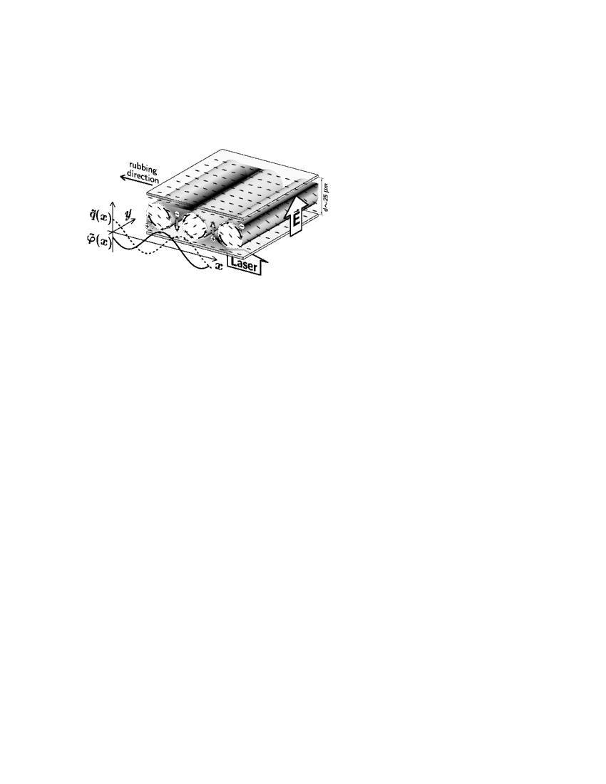
Figure 1: Schematic drawing of the convection rolls and director field in a nematic sandwich cell. A snapshot of the spatial modulations of director and charge fields $(\tilde{\varphi},\tilde{q})$ in the cell midplane is sketched.

The experimental geometry is sketched in Fig. 1. The ground state with the nematic director (optic axis) uniform along an easy axis in the cell plane is achieved by proper surface treatment of the cell plates. An electric field is applied normal to the cell plane. Nematic material with negative dielectric anisotropy $\Delta\epsilon$ is chosen to prevent the splay Fréedericksz instability. In the electric field, the dielectric torque stabilizes the ground state, but small thermal fluctuations of the director field in connection with an anisotropic conductivity of the nematic generate a periodic space charge modulation in the cell plane. The interaction of these space charges with the electric field lead to convective flow which in turn generates a destabilizing viscous torque on the director field. Above a threshold voltage U${}_{\text{c}}$, this torque exceeds the stabilizing dielectric and elastic torques and a periodic pattern of convection rolls and corresponding director deflections is formed. In the simplest case, the wave vector of the first instability is along the director (normal rolls). The roll structure appears in optical transmission as an array of parallel stripes in the cell plane (Fig. 1).

Electroconvection is conventionally driven with a periodic AC voltage (to avoid sample degradation in DC fields). For the understanding of the mechanism of pattern formation it is essential to note that director and charge fields respond on different time scales to the alternation of the electric field. The symmetry of the dynamic equations requires that their time dependence with respect to a periodic driving field is antisymmetric. This is reflected in the existence of two different types of patterns. In the low frequency ’conduction’ regime, charge relaxation is fast compared to the AC frequency. The charge density alters its sign with the applied field, the sign of the director deflection is preserved. The voltage for the onset of conduction rolls increases monotonously with frequency. At the cut-off frequency $f_{c}$, the threshold voltage curve intersects that of the ’dielectric’ patterns. In the dielectric regime above $f_{c}$, the director deflections alternate with the field while the charge density modulation retains its sign. Figure 2 shows the stability diagram for the system studied in this paper. Figure 2(a) gives the onset voltage for the first instability, towards normal rolls. The corresponding wave numbers are shown in Figure 2(b).

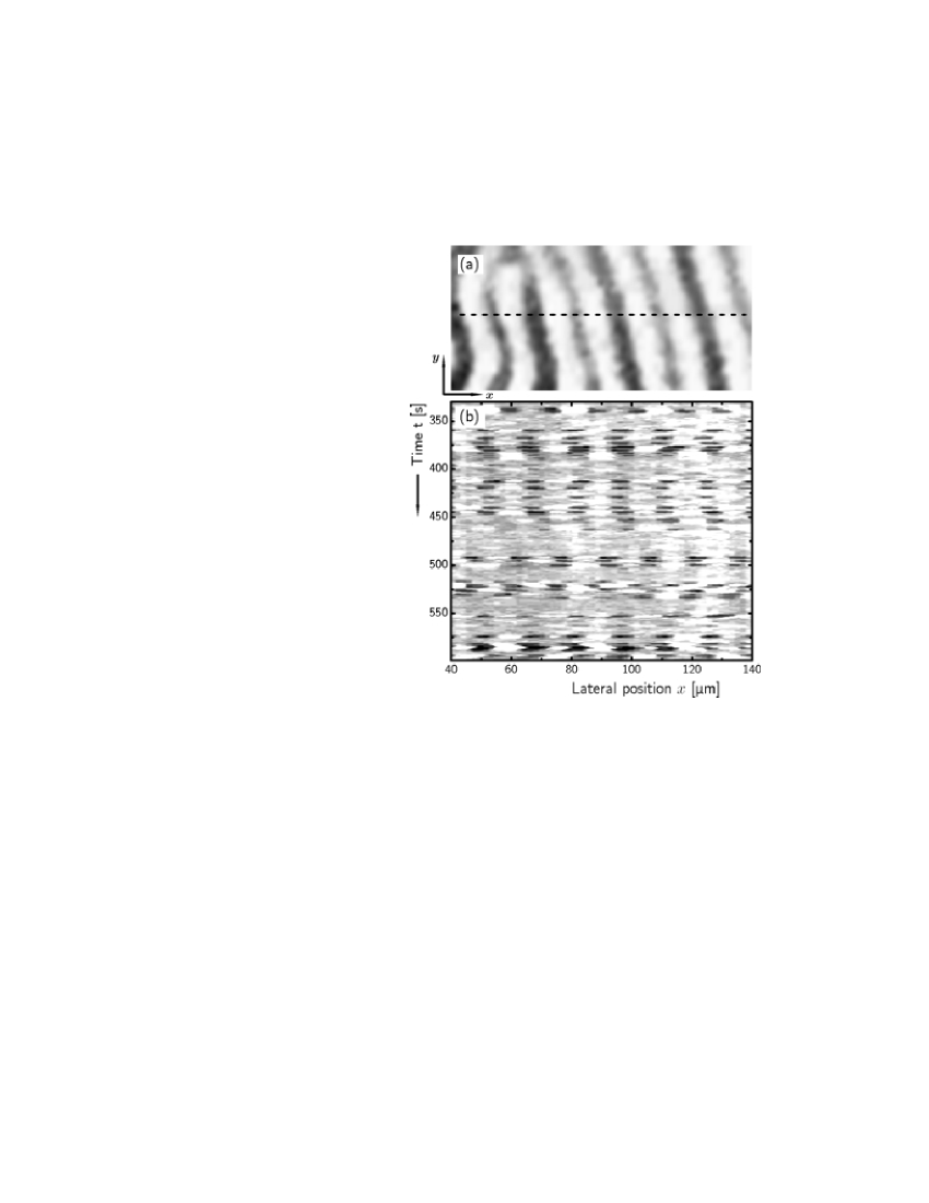
Figure 3: Transmission microscope images of the noise driven pattern during a burst (a) and space-time plot of a cross section along the wave vector (b). The horizontal axis gives the spatial coordinate along the pattern wave vector (director easy axis). Only in adjacent bursts, the spatial phase of the pattern appears correlated, long laminar phases destroy such correlations.

When a stochastic excitation scheme is used where the driving field has no deterministic component (as e.g. the dichotomous Markov process that is considered in this paper) the system does not exhibit a sharp transition from the quiescent to the convective state upon variation of the control parameter but shows intermittent behaviour. Two different regimes are found which have many features in common with the corresponding conductive and dielectric regimes in the deterministic case. At onset of the instability, one of the system’s characteristic times (director or charge relaxation) becomes comparable to the characteristic time of the noise $\tau_{stoch}$. A considerable qualitative change of onset and appearance of the convection patterns Brand85 ; amm97 is observed. A typical snapshot is shown in Fig. 3.

Nevertheless, there was little interest until recently in the quantitative statistical interpretation of the structures at the instability threshold. Main focus of research has been directed to the study of superimposed deterministic and stochastic driving fields and the construction of pattern state diagrams. The empirical concept of a threshold voltage has been applied in previous experimental investigations of noise driven EHC Kai79 ; Kawa81 ; Brand85 ; Kai87a ; Kai87b ; Kai89b and statistical methods have been applied to test various stability criteria Behn85a ; Behn85b ; Behn85c ; Behn85d ; Behn98 . The largest Lyapunov exponent $\lambda$ of the trajectories of the system variables, which is analytically known Behn98 , provides a quantitative measure for the instability threshold, but the crucial problem is the experimental determination of the threshold in a system with limited dynamical range and additive noise. The statistical analysis of the intermittent trajectories provides an experimental tool to characterize the stability threshold, $\lambda=0$ John .

The observation and quantitative characterization of the dissipative patterns under stochastic excitation is achieved in this study by exploring the phase grating formed by the spatially periodic deformed director field. The laser scattering profile resulting from the nematic convection patterns is recorded. A two-dimensional (2D) detector allows to observe the complete scattering profile of the transmitted laser light and to study the wave vector orientation and wavelength selection process with a sampling rate of 25 s^-1, and alternatively a photo diode positioned at the scattering reflex enables us to record the trajectory of the dominant mode with faster sampling rate and higher intensity resolution.

II Sample preparation and Experiments

II.1 Sample preparation

We use the nematic mixture Mischung 5 (Halle) which consists of four disubstituted alkyl(oxy)phenyl-alkyloxybenzoates. This material has been used in previous EHC experiments John ; amm97 ; amm98 ; bohatsch . The mixture is nematic at room temperature, its clearing point is 70.5 ^∘C. The commercial sandwich cells (LINKAM) used in the experiments have cell gaps of 25.8 $\mu$m. The glass plates are covered with transparent Indium-Tin-Oxide electrodes (5 mm$\times$5 mm), they are polyimide coated and antiparallelly rubbed for planar surface alignment. The temperature of the samples is controlled by a Linkam heating stage with an accuracy of 0.1 K. The sample temperature has been set to 32^∘C in all experiments.

II.2 Material Parameters

All relevant material parameters for the simulation of the electrohydrodynamic equations except for some viscosities have been measured in independent experiments amm99 ; MGRS . The conductivity of the nematic samples differs by about 20% between individual cells, values for a given cell are almost constant in time. In order to prevent long-term trends of the conductivity, we reheat the material into the liquid phase between subsequent runs of the experiment, similar procedures have been proposed in Bisang98 ; Bisang99 . All measurements presented in the diagrams of this paper have been performed consecutively with the same cell, in order to obtain quantitatively comparable results for the different statistical investigations. Differences in conductivity between individual cells may lead to variations of the respective thresholds but do not influence the statistical characteristics.

In order to complete the parameter set for the numerical simulations, we fitted the threshold curves and critical wave numbers for deterministic square wave excitation where the experiment yields sharp thresholds towards the first instability. With a fixed parameters set (Table I), good agreement between numerical results and experimental data is achieved across the whole frequency range investigated (Fig. 2). The same parameter set is used thereafter for the calculation of the Lyapunov exponents and stochastic trajectories.

II.3 Excitation

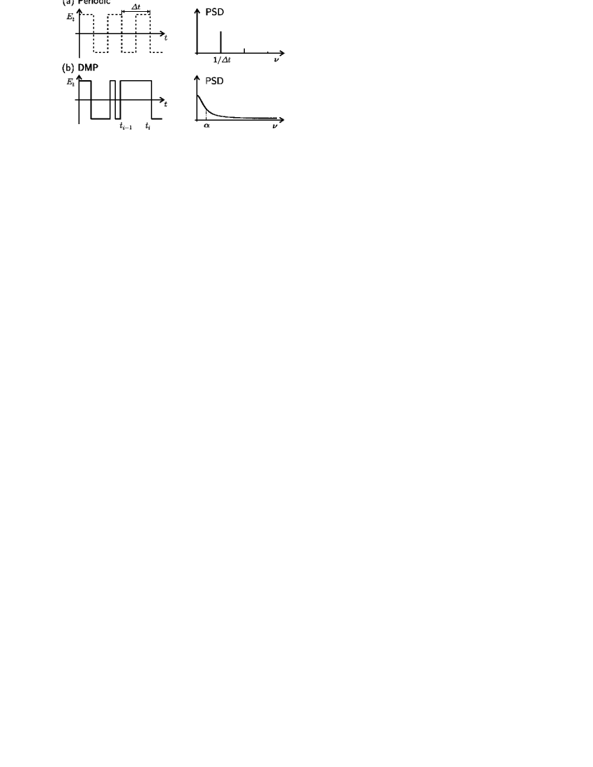
Figure 4: Excitation waveforms and corresponding power spectral densities for periodic square wave (a) and DMP (b).

The waveform of the driving electrical voltage is synthesized by a computer and subsequently amplified. We generate the driving voltage curve with a sampling rate of 10 kHz. Although the spectrum of this waveform is in principle discrete, we can consider it as quasi-continuous in the frequency range relevant in the experiments (below $500$ Hz). Within this study, we have used a few special waveforms, which are detailed in the following, Figure 4 visualizes their signal shapes and shows the respective power spectra.

Periodic square wave excitation is used to construct the stability diagram for deterministic driving. We exploit the sharp threshold towards the first instability for the adjustment of system parameters and test of the long term stability of the samples. For example, the cut-off frequency is a sensitive measure to reveal even small changes of the sample conductivity.

The Dichotomous Markov process (DMP) is the stochastic waveform used in all experiments presented below. It is characterized by random jumps of the electric field between the two values ${+E}$ and ${-E}$, with an average jump rate $\alpha$. The time intervals between consecutively jumps are distributed as $\Delta t_{i}=-1/\alpha\,\ln x_{i}$, where $x_{i}\in(0,1]$ is a uniformly distributed random number. In analogy to a deterministic square wave excitation with frequency $\nu$, we define the ’average frequency’ $\nu=\alpha/2$. The DMP power spectrum is Lorentzian with its maximum at frequenzy zero and a half width related to the jump rate by $\alpha/\pi$ (Fig. 4(b)). An important feature that facilitates the numerical calculations is that all terms quadratic in the electric field are time independent in the DMP. An analytical calculation of the sample stability threshold and the critical wave numbers have been performed Behn98 . Technically, identical realizations of the stochastic process can be reproduced with the computer. This allows us to use identical noise sequences for experiment and simulations when details of the trajectories of pattern amplitudes are of interest.

Other stochastic processes have been tested in additional experiments. While the DMP randomizes the phases of a periodic square wave, another stochastic process can be synthesized that randomizes the amplitudes of the square wave but keeps the jumps equidistant. This randomization of the amplitude can be combined with a random phase of the jumps. Such processes do not complicate the numerical simulations, the electric field is piecewise constant and the equations of motion can be integrated straightforwardly. It turns out that the statistical properties of the trajectories and the derived scaling laws for these stochastic processes are in full accordance with those for the DMP. Therefore, we will discuss only the DMP results being representative for other types of stochastic excitation.

II.4 Data acquisition

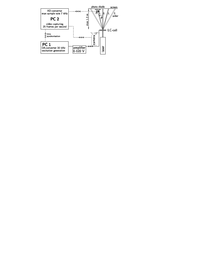
Figure 5: Sketch of the experimental setup.

The sample cell is irradiated by a He-Ne laser with wavelength $\lambda_{\text{laser}}$=632.8 nm at normal incidence. The beam diameter is about 1 mm. The scattered light is monitored on a screen in a distance of maximum 1.3 m from the cell (Fig. 5). When the sample is in the ground state (zero electric field), only a weak background scattering $A_{0}(t)$ is observed around the primary beam. Since we are interested in scattering from spatially deformations of the director field, we correct the raw data with a time averaged intensity $\overline{A_{0}}$ by $A(t)=|A_{\text{raw}}(t)-\overline{A_{0}}|$. This correction is marginal since the background signal is in general three orders of magnitude smaller than the amplitude of the scattering reflex at the position of the photo diode.

From the two-dimensional scattering images, wavelengths and orientations of the patterns can in principle be continuously extracted. However, because of bandwidth limitations in signal processing we use two different equipments to record the scattering data.

A commercial video camera is employed to take 2D scattering images with an acquisition rate of 25 frames per second and 8 bit intensity resolution. This enables us to study the evolution of the mode spectrum and to access the full wave vector information, although time and intensity resolution are limited.

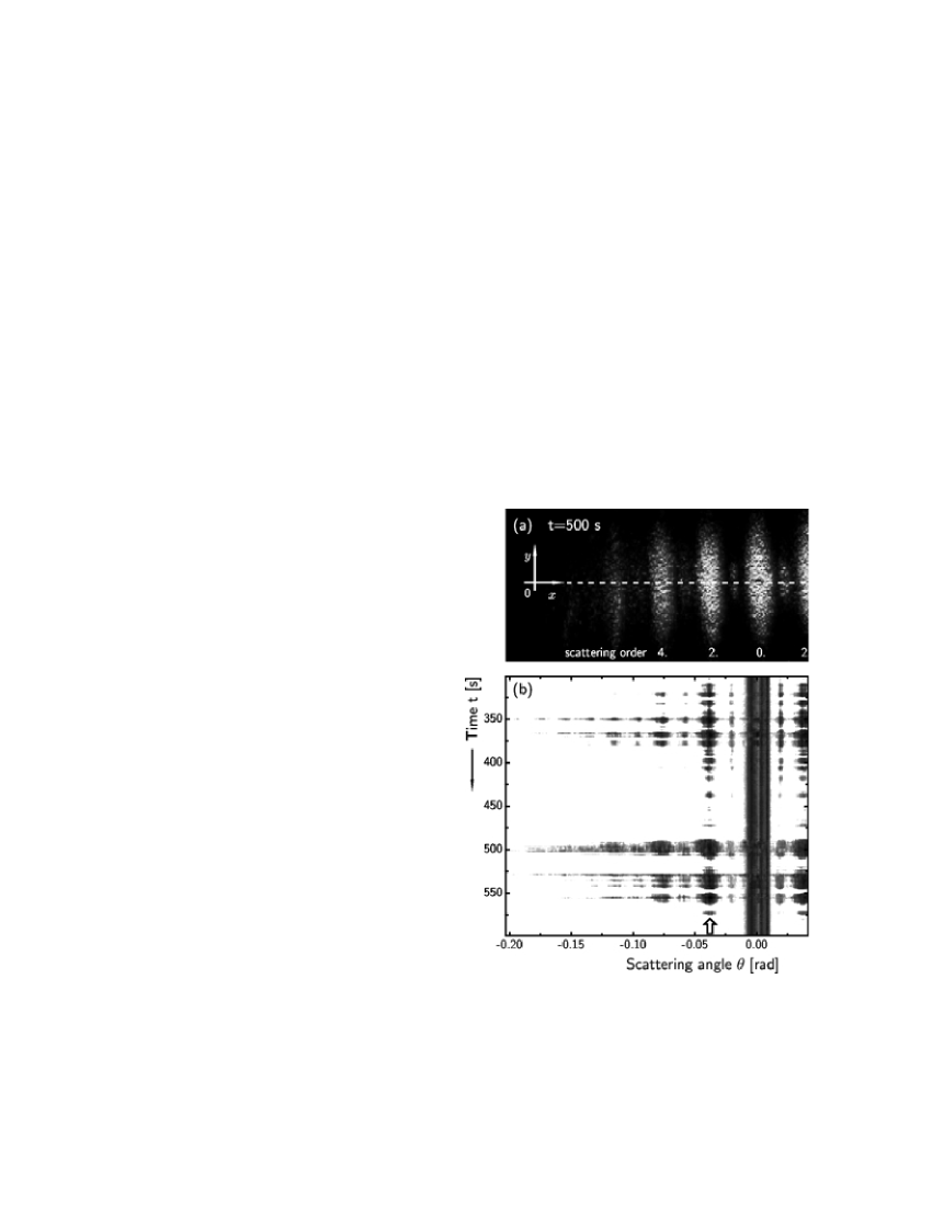
Figure 6: Scattering image at $\alpha=2\nu=160$ s^-1 (jumps per sec) DMP excitation recorded with CCD camera. (a) 2D snapshot during an intensive burst at $t=500$ s, (b) scattering angle-time plot of intensity profiles taken at $y=0$, presented in inverse grey scale. The constant angles of the individual reflexes in subsequent bursts reflects the fast and stable wavelength selection mechanism. An arrow marks the position of the photo diode, set to the most intense scattering reflex of the most instable wave number.

The 2D images show that at given frequency, the pattern is dominated by a single mode (see Fig. 6) with fixed wave vector but varying amplitude. Any low order scattering reflex of that mode is representative for the momentary pattern, and it is sufficient to record only the scattering intensity at a fixed position (here, we use one of the two symmetric second order reflexes). For that purpose we employ a photo diode with aperture 7 mm² adjusted to the reflex of interest.

The photo diode signal is digitized and the trajectory is stored in a computer. We use a fast (0.2 ms time resolution) 12 bit AD concerter for measurements with high time resolution as for example the determination of laminar phases, and alternatively a slow (0.1 s) 24 bit ADC for accurate amplitude measurements over large dynamic ranges.

III Optics

The electroconvection rolls in the nematic material produce spatial periodic director deflections

$$\tilde{\varphi}(x,z,t)=\varphi(t)\sin(k_{x}\,x)\sin(k_{z}\,z)$$ (1)

which lead to a modulation of the effective refractive index $n_{\text{eff}}$ for the transmitted extraordinary beam,

$$n_{\text{eff}}(\beta(x,z))=\frac{n_{o}\,n_{e}}{\sqrt{n_{o}^{2}\cos^{2}\beta(x,z)+n_{e}^{2}\sin^{2}\beta(x,z)}},$$ (2)

where $n_{o},n_{e}$ are material parameters and $\beta$ is associated with the angle between the light ray and an optical axis Rasenat89 . A phase and amplitude grating is formed in the cell. There has been some discrepancy in literature about the usage of refractive or ray index in these calculations. For the small fluctuations considered here, both approximations lead to similar results. In order to establish a relation between the experimental observations and the results of the simulations of the director and charge fields, it is necessary to calculate the diffraction efficiency of a given periodic director field. We use the eigenfunctions $\tilde{\varphi}(x,z,t)$ from the linear stability analysis. Using Fermat’s principle it is possible to determine the optical path, the resulting phase difference $\phi(x,t)$ and the intensity profile of light passing the cell Rasenat89 ; vistin ; kondo ; kondo2 ; rehberg3 ; kosmopoulos ; joets1 ; joets2 . At small deflection angles, one can assume that individual light rays pass the cell without deflection, creating a phase grating

$$\phi(x,t)=\frac{2\pi}{\lambda_{\text{laser}}}\int_{0}^{d}n_{\text{eff}}\,\text{d}z\approx$$ (3)

$$\int_{0}^{\pi/k_{z}}\frac{2\pi n_{e}}{\lambda_{\text{laser}}}\left[1-\frac{n_{e}^{2}-n_{o}^{2}}{2n_{o}^{2}}\varphi(t)^{2}\cos^{2}(k_{x}x)\sin^{2}(k_{z}z)\right]\text{d}z.$$

Analytical integration over $z$ along a straight path through the cell Caroll72 yields a periodic phase modulation $\Delta\phi(x,t)$ with twice the wave number $k_{x}$ and a quadratic dependence on the director deflection

$$\Delta\phi(x,t) = \frac{n_{e}\,\pi^{2}\text{ }(n_{e}^{2}-n_{o}^{2})}{2n_{o}^{2}\,k_{z}\lambda_{\text{laser}}}\varphi(t)^{2}\cos^{2}(k_{x}x)$$ (4)

$$\propto \varphi(t)^{2}\cos^{2}(k_{x}x)\propto\,\varphi(t)^{2}\cos(2\,k_{x}x).$$

In this approximation, the intensity modulation with $k_{x}$ due to focussing effects of the inhomogeneous refractive index profile is neglected and only even order reflexes appear in the scattering image. This is in agreement with the experimental observations. The second order reflex dominates the small amplitude patterns, and with increasing amplitude of the director deflections $\varphi(t)$, higher order reflexes can be observed. We note that the amplitude grating (which produces the well known shadowgraph images in conventional orthoscopic microscopy) is effective as well, it is most prominently reflected in the weak first order reflexes (see Fig. 6).

The relation $k_{x}=2\pi\sin\theta_{m}/(m\lambda_{\text{laser}})$ connects the scattering angle $\theta_{m}$ of the $m$th order reflex with the wave number $k_{x}(\theta_{m})$. The scattered light intensity $A(t)$ of the phase grating at the second order reflex is related to the square of the Bessel function of first kind, $J_{1}(\phi_{\max}(t))$, with the amplitude of the phase grating $\phi_{\max}$ in the argument Caroll72 ; Kashnow72 ; Papadopoulos99 ; Bouvier00 ; Zenginoglou89 ; Smith77 . For small director deflections $\varphi(t)$, the intensity at the second order reflex is proportional to the fourth power of $\varphi$

$$A(t)\propto J_{1}^{2}(\phi_{\max}(t))\propto\phi_{\max}^{2}(t)\propto\varphi^{4}(t).$$ (5)

By numerical integration of the nonlinear Euler-Lagrange equations we have calculated the actual propagation of light beams through the sample. The numerical integration allows for the deflection of light and thus for intensity modulations by focussing effects. These simulations confirm the relation $A(t)\propto\varphi(t)^{4}$ even for large director deflections $\varphi(t)\lesssim 1$.

The numerical simulation of EHC patterns yields $\psi=\partial_{x}\varphi$, (see below) which represents the director deflection for a given mode. For comparison of simulated $\varphi$ and experimental intensities we use the relation

$$A^{\text{th}}(t)=\text{const}\varphi^{4}(t).$$ (6)

We emphasize that we compare the experimental and simulated pattern amplitudes only on a relative level, since no efforts have been made to relate calculated absolute scattering intensities to voltages measured by the photosensor. Since the simulations use a linear model, absolute scaling of pattern amplitudes is not relevant for the fundamental statistical properties of the system.

IV Numerical simulations

Basic Equations

The basic equations for the charge and director fields and the method for analytical derivation of the Lyapunov exponents in the electrohydrodynamic instability have been described in detail in Behn98 .

The important quantities describing the system dynamics are the charge density $\tilde{q}$ and the amplitude of the director deflection $\tilde{\varphi}$ (see Fig. 1). A standard technique to describe the time evolution of small amplitude periodic patterns is the use of linearized differential equations and a two-dimensional mode ansatz for the two involved quantities,

$$\tilde{\varphi}(x,z,t) = \varphi(t)\sin(k_{x}\,x)\sin(k_{z}\,z),$$ (7)

$$\tilde{q}(x,z,t) = q(t)\cos(k_{x}\,x)\sin(k_{z}\,z).$$ (8)

In the relevant parameter range, the pattern is spatially periodic along the director easy axis ($x$ direction) This result of the linear stability analysis is in agreement with the experimental observations. Therefore, we consider only the stability of modes with the wave vector parallel to the $x$ axis. The (stress free) boundary conditions for the director field at the glass plates $\tilde{\varphi}(z=0)=\tilde{\varphi}(z=d)=0$ are satisfied by $k_{z}=\pi/d.$ For convenience, the director deflection $\tilde{\varphi}$ is substituted by the curvature $\tilde{\psi}=\partial_{x}\tilde{\varphi}$. A system of two ordinary differential equations is derived from the torque balance, Navier-Stokes and Maxwell equations. After linearization we obtain an ordinary differential equation system in time for the vector ${\bf z}\left(t\right)=(q\left(t\right),\psi\left(t\right))^{T}$,

$$\frac{\text{d}}{\text{d}t}{\bf z}\left(t\right)=-\left(\begin{array}[]{cc}1/T_{q}&\sigma_{\text{H}}E(t)\\ aE(t)&\Lambda_{1}-\Lambda_{2}E(t)^{2}\end{array}\right){\bf z}(t),$$ (9)

where $\Lambda_{1},\Lambda_{2},T_{q},\sigma_{H}$ and $a$ are parameters related to the viscous, elastic and electric properties of the liquid crystal as well as to the wavelength $k_{x}$ of the modes Behn98 . The electric field amplitude $E(t)$ $=$U$(t)/d$ corresponds to the excitation voltage U$(t)$. In case of piecewise constant excitation (as the deterministic square wave and DMP described above), $E(t)$ assume only two values $\pm E$, and all elements of the matrix are constant between consecutive jumps. Within a time interval $\Delta t_{i}$ of constant excitation field, integration of the differential equation gives a solution in the form of a sum of two exponentials. The solution ${\bf z}_{i}$ from the $i$th integration step is taken as the starting value for the $(i+1)$st step. The complete trajectory for given $k_{x}$, $E$ and set of (random) times $\Delta t_{i}$ for jumps of the excitation voltage is calculated with an initial vector ${\bf z}_{0}=(q,\psi)|_{t=0}$. At the discrete jump times $t_{n}$, the solution is

$${\bf z}(t_{n}) = {\bf T}^{(s_{n})}(\Delta t_{n})\cdots{\bf T}^{(s_{1})}(\Delta t_{1})\;{\bf z}(0),$$ (10)

$$\Delta t_{i} = t_{i}-t_{i-1}\;;\;s_{i}=\text{sign}\,E(t_{i}>t>t_{i-1}),$$

$${\cal T}_{n} = \prod_{i=1}^{n}\,{\bf T}^{(s_{i})}(\Delta t_{i}),$$ (11)

where ${\bf T}^{(s_{i})}(\Delta t_{i})$ is the 2$\times$2 time evolution matrix for the $i$th interval.

For a detailed statistical analysis of $\psi(t),$ in particular for the calculation of power spectral densities (PSD), the trajectory can be filled in the intervals between the jumps using the exact exponential solutions ${\bf T}^{(s_{i})}(t-t_{i-1})$.

In the particular system studied here, the eigenvalues ${\bf Eigenval}{}\,{\cal T}_{n}(E,k_{x})$ are real and positive. For periodic square wave driving, all intervals $\Delta t_{i}$ are equal and the product is ${\cal T}_{n}=(T^{+}T^{-})^{n/2}$. For the calculation of the Lyapunov exponents it is sufficient to consider ${\bf Eigenval}{}\,(T^{+}T^{-})$. This reproduces the well known results of classical theory using Floquet methods orsay ; duboisviolette .

In the case of stochastic excitation all the $\Delta t_{i}$ are different and the calculation of the Lyapunov exponents leads to an infinite product of 2$\times$2 random matrices Behn98 . This system yields two real Lyapunov exponents $\lambda_{1}>\lambda_{2}$ which are related to the eigenvalues of the product of stochastic matrices ${\cal T}_{n}$. In particular, the largest Lyapunov exponent (in the following denoted by $\lambda$) is found from

$$\lambda=\lim_{n\rightarrow\infty}\frac{1}{t_{n}}\ln\{\max({\bf Eigenval}{}\,{\cal T}_{n})\}.$$ (12)

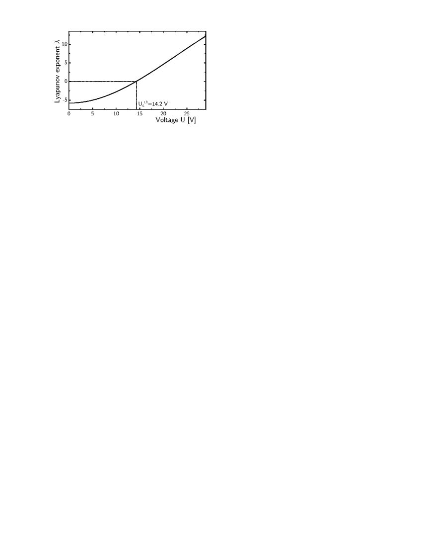
Figure 7: Analytically calculated Lyapunov exponent $\lambda$ of the most instable mode, $k_{c}=0.204$ $\mu$m^-1, for DMP excitation with $\nu=80$ s^-1. Material parameters are taken from the fit of periodic excitation thresholds and wavelengths. The value $\lambda=0$ defines the critical voltage $\text{U}_{\text{c}}^{\text{th}}=14.2$ V.

For DMP excitation, the Lyapunov exponents can be obtained analytically Behn98 . Figure 7 shows the Lyapunov exponent for the critical wave length calculated with the parameters specified above. In the linear model, $|{\bf z}|$ is growing to infinity ($\lambda>0$) or shrinking to zero ($\lambda<0$), depending on the value of the largest Lyapunov exponent. The selected wavelengths and threshold voltages for a given frequency and set of material parameters are calculated from the neutral curve. The wave number is varied and the minimum $E_{c}$ of the neutral curve provides the critical wave number $k_{c}$.

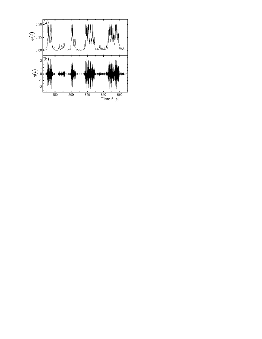
Figure 8: Details of a simulated trajectory of $\psi$ and $q$ at $\nu=80$ s^-1, at $\lambda=0$ (’conductive’ regime) for a constant lower boundary $\psi_{\min}=5\times 10^{-3}$, see Eq. (13). In the low frequency regime the slow variable $\psi(t)$ keeps its sign, whereas $q(t)$ oscillates synchronously with the applied field $E_{t}$.

Because of the symmetries of Eq. (9), one of the system variables ($q,\psi$) keeps its sign while the other variable has to change its sign with the polarity of the applied field. At periodic excitation, the system is synchronized with the applied field and the conduction ($q$ alternating periodically) and dielectric ($\psi$ alternating periodically) regimes are distinguished. In case of DMP excitation, the support of one of the variables still preserves the sign and the two regimes can still be distinguished Behn98 . In the following, we will discuss only the low frequency conduction regime, Fig. 8 shows details of a simulated trajectory. The slow variable is the director deflection which is directly related to the measured quantity, the scattering intensity. Due to the coupling of ($q,\psi$), both the director deflection and the envelope of the charge density curves show the same long term ($t>1/\nu$) characteristics.

Boundaries

In the linear description, the trajectories tend to infinity or zero for all values of $\lambda\neq 0$. However, a realistic description of the experiments has to consider boundaries for ${\bf z}$. Nonlinearities in the system limit the excursion of the system variables ${\bf z}$ to large values while additive noise prevents their unlimited decay. In order to compare the results of simulations and experiments, we introduce limits for the director deflection (curvature $\psi$) by clipping each time step

$$\psi(t_{i})=\begin{cases}\psi_{\max}&\text{if $\psi(t_{i})>\psi_{\max}$},\\ \psi_{\min}&\text{if $\psi(t_{i})<\psi_{\min}$},\\ \psi(t_{i})&\text{else}.\end{cases}$$ (13)

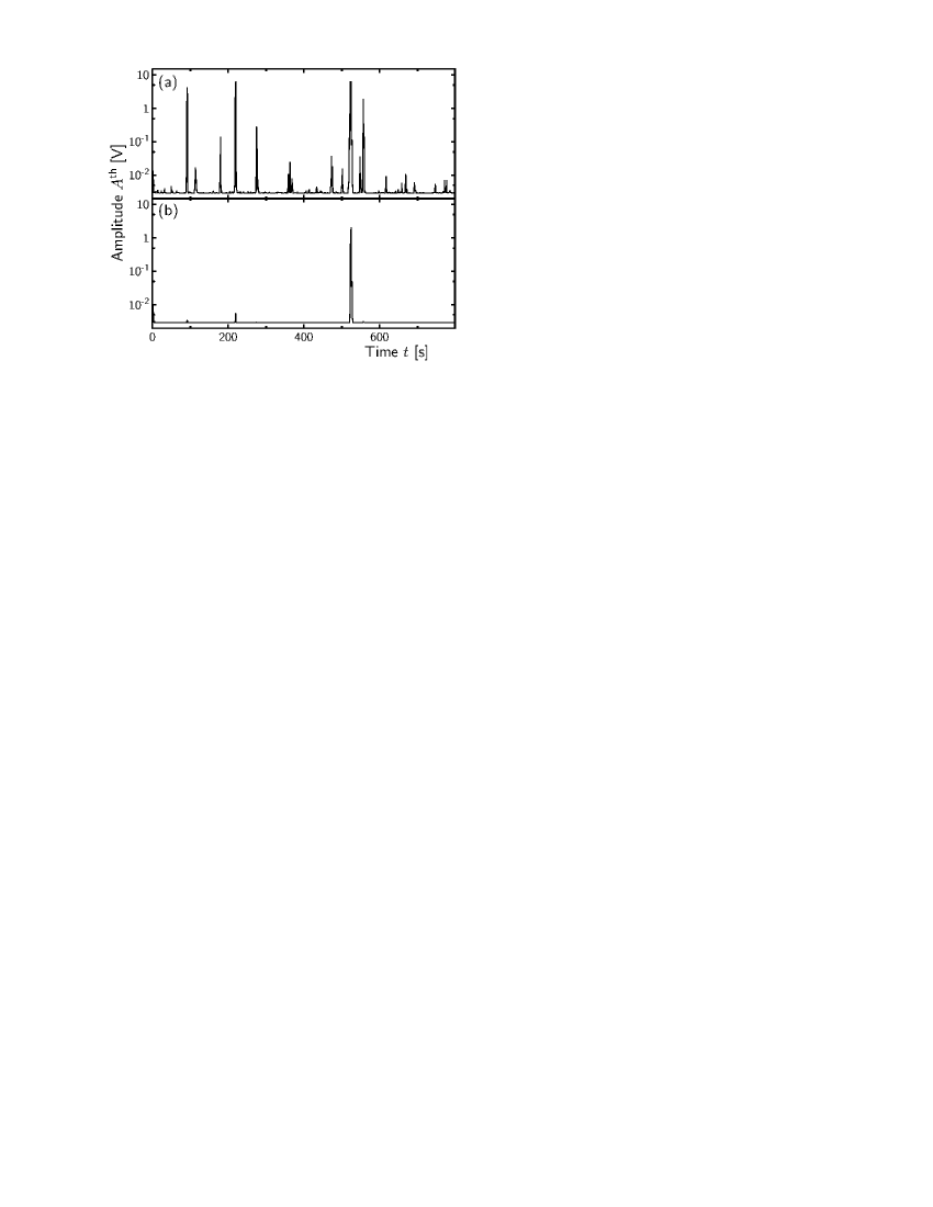
Figure 9: Two simulated trajectories at $\lambda<0$ for different constant background levels (a) $\psi_{\min}=5\times 10^{3}$ and (b) $\psi_{\min}=5\times 10^{4}$. The trajectories appear to be significantly different, whereas the statistical analysis produce the same fundamental power laws.

Because of the linearity of the ODE system (Eq. (9)), only the ratio of the upper and lower thresholds is important. A constant factor in the amplitudes is irrelevant for the statistical properties and scaling laws. Here, we assume that the dynamic range is two orders of magnitude, $5\times 10^{-3}<\psi(t_{i})<0.5$. This dynamical range reflects approximately the situation of a thermal background stimulation $\langle\varphi^{2}\rangle^{1/2}\sim\gamma_{1}/K_{11}k_{x}^{2}\sim 5$ mrad Bisang99 ; Bisang98 ; Rehberg91 and an upper limit of 0.5 rad. For negative Lyapunov exponents, the lower boundary is necessary to prevent the unlimited decay of $\psi(t)$. The choice of the value of the lower boundary has strong effect to the number of burst per unit time (see Fig. 9), but only small effects on the fundamental statistical laws (see below).

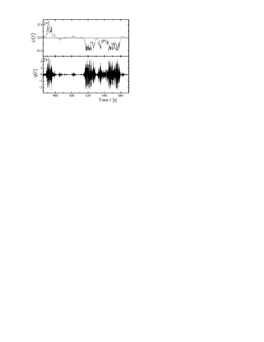
Figure 10: Same as in Fig. 8 but with background additive noise in $\psi(t)$. With additive noise, $\psi(t)$ can change its sign occasionally. The pattern amplitude as well as the optical scattering intensities are, however, insensitive to the sign of $\psi$.

The assumption of a well defined lower limit is of course artificial and cannot describe the actual experimental behaviour for very small pattern amplitudes. A more realistic assumption considers low amplitude additive noise in the variable $\psi(t_{i})$. We have studied this case by adding Gaussian random numbers with a given variance $D$ Fox88 at each time step. For zero electric field, Eqs. (9) decouple and $\psi$ describes an Ornstein-Uhlenbeck process (OUP) which is characterized only by $D$ and the exponentially decaying autocorrelation with the correlation time $\tau_{\text{OUP}}\propto 1/\lambda$ related to the Lyapunov exponent at zero voltage (see Fig. 7). One consequence of such additive noise is that the simulated trajectories for the slow variable $\psi(t)$ can change sign (see Fig. 10), in contrast to Eq. (13). This is not relevant for the comparison with the scattering experiment which is insensitive for the spatial phase of the pattern. If the variance $D$ is chosen such that the mean square amplitude of $\psi$ in absence of electric fields gives $\langle\psi^{2}\rangle^{1/2}=\psi_{\min}$, the statistical properties of $|\psi|$ are qualitatively identical with the simulations using conditions (13).

V Results and Discussion

V.1 Pattern images

The conventional technique to observe pattern formation in EHC is the shadowgraph method Rasenat89 in combination with a transmission microscope. An instant picture of a pattern burst, recorded by means of orthoscopic microscopy, is shown in Fig. 3(a). The dynamics of this pattern can be visualized best when the intensity in a cross section perpendicular to the rolls is scanned and a spatio-temporal plot as in Fig. 3(b) is analyzed. Some bursts, in particular those which appear in fast sequence, are correlated in their spatial phase. After long laminar phases, however, there is in general no spatial correlation remaining between the bursts. For stationary rolls, this loss of correlation is a consequence of additive noise in the system, it triggers new modes whenever the pattern amplitude reaches thermal noise level. In such cases, the new fluctuation mode has an arbitrary spatial phase with respect to the previous convection pattern. On the other hand, there are sequences of bursts in Fig. 3(b) which preserve spatial correlation. They can be attributed to amplifications of the same mode which has disappeared in the optical image but has not reached the level of additive noise during the intermediate laminar phase.

V.2 Scattering images

Figure 6(a) shows a snapshot of the scattering image originating from a burst in a DMP driven d=25.8 $\mu$m thick nematic cell, taken with the 2D camera detector. The image shows the primary beam at $\theta=0$ and diffuse scattering spots from the periodic spatial director modulation in the cell. The scattering reflexes concentrate on the $k_{x}$ axis, i.e. normal electroconvection rolls are observed. A wave number $k_{x}$ of the pattern producing this image of 0.2 $\mu$m^-1 is derived from the spot positions, the director period is $\lambda_{dir}=2\pi/k_{x}=32$ $\mu$m. Below the scattering image, in Fig 6(b), the time dependence of the intensity profile taken along the horizontal symmetry axis of the profile ($k_{y}=0$) is plotted. For better reproduction, the image is plotted with inverse gray scale, dark spots correspond to high amplitudes of scattered light and consequently to large director modulations (bursts). The bursts are characterized by a narrow wavelength band and the reflexes remain approximately at the same positions, i.e. in all bursts the patterns have nearly the same wavelengths. The wavelength selection process itself is not observable in the images, it is obviously fast compared to the video rate of 25 Hz and occurs below the level of optical sensitivity of our camera. The information about the spatial phase of the patterns gets lost in the scattering image, therefore we cannot determine from the scattering images whether the convection rolls of subsequent bursts appear spatially phase correlated or not. The essential information taken from the 2D images is that the wavelength of the noise driven patterns is constant and the scattering image consists of reflexes at fixed scattering angles with varying amplitudes. Thus, we achieve a considerable data reduction by restricting to the strongest scattering reflex. In particular, the detector is placed at the second order scattering reflex of the most critical wave number, indicated by the arrow in Fig. 6(b).

V.3 Trajectories

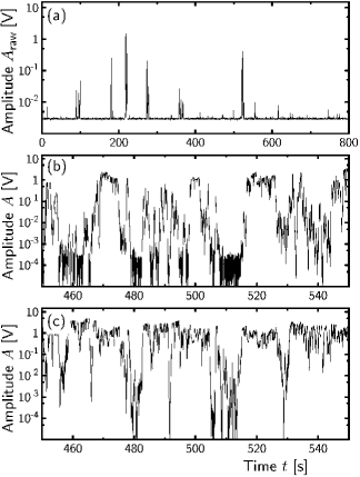
Figure 11: Trajectories recorded with a photo diode positioned at the most intense second order reflex and 24 bit ADC, the excitation is identical with that in Fig. 6. (a) At low voltage (U=12.2 V) the measured raw signal $A_{\text{raw}}$ fluctuates around a background level $\overline{A_{0}}$, interrupted by infrequent bursts. (b) Corrected intensity $A(t)=|A_{\text{raw}}(t)-\overline{A_{0}}|$ at U=12.9 V where we assume $\lambda=0$ (see statistical analysis). The up-down symmetry of the curve is recognized. The experimental dynamic range is limited by saturation for large amplitudes and by background noise for small amplitudes. (c) At U=13.6 V the on-state is dominant, intermitted infrequently by breakdowns to the quiescent off-state.

The intensity of scattered light at the position of the second order scattering reflex of the first unstable mode is shown in Fig. 11. The curves have been digitized by means of the 24 bit AD converter. The random electric excitation field $E_{t}$ uses identical realizations of the stochastic process for all three trajectories, with different amplitudes $E$. Concerning the effects of the multiplicative noise in the system, details of the three curves can be directly compared. The characteristic frequency $\nu$ was 80 Hz, corresponding to an average of 160 jumps/s of the sign of $E_{t}$. Fig. 11(a) shows the raw signal from the detector for a voltage below the critical U${}_{\text{c}}^{\text{exp}}$. The contributions of (additive) background fluctuations to the detector signal are of the order of $10^{-3}$ V around a constant offset $\overline{A_{0}}=3\times 10^{-3}$ V. Bursts of the spatially periodic pattern that exceed the background noise level occur infrequently. From arguments discussed in the next sections we conclude that the excitation voltage is below the stability threshold (defined by the Lyapunov exponent $\lambda=0$). In Fig. 11(b), the voltage is approximately equal to the critical voltage ($\lambda=0$). The characteristic feature of the trajectory is its mirror symmetry of high and low amplitude excursions of the scattering intensity $A(t)$ on logarithmic scale. Rise and decay sections of the graph are symmetric. We note that in a linear presentation of the same plot $A(t)$, the high amplitudes will appear as prominent bursts out of the background level, and the typical intermittent behavior is acknowledged. At higher voltages (Fig. 11(c)), the trajectory will be predominantly in the saturation region (’on’ state), interrupted by short laminar phases. These intrinsic symmetries reflect theoretical predictions for on-off intermittent behaviour Cenys97 .

Amplitudes in Figs. 11(b,c) have been corrected for the background intensity, $A=|A_{\text{raw}}-\overline{A_{0}}|$. This correction attempts to separate the constant (stray light) background signal and additive (thermal) noise in the trajectories. Since these contributions are comparably small, the correction effects only the low amplitude sections of the trajectories. It faciliates the identification of laminar phases and enables us to visualize the symmetry of burst and quiescent periods in the logarithmic scale.

V.4 Distribution of Laminar Phases

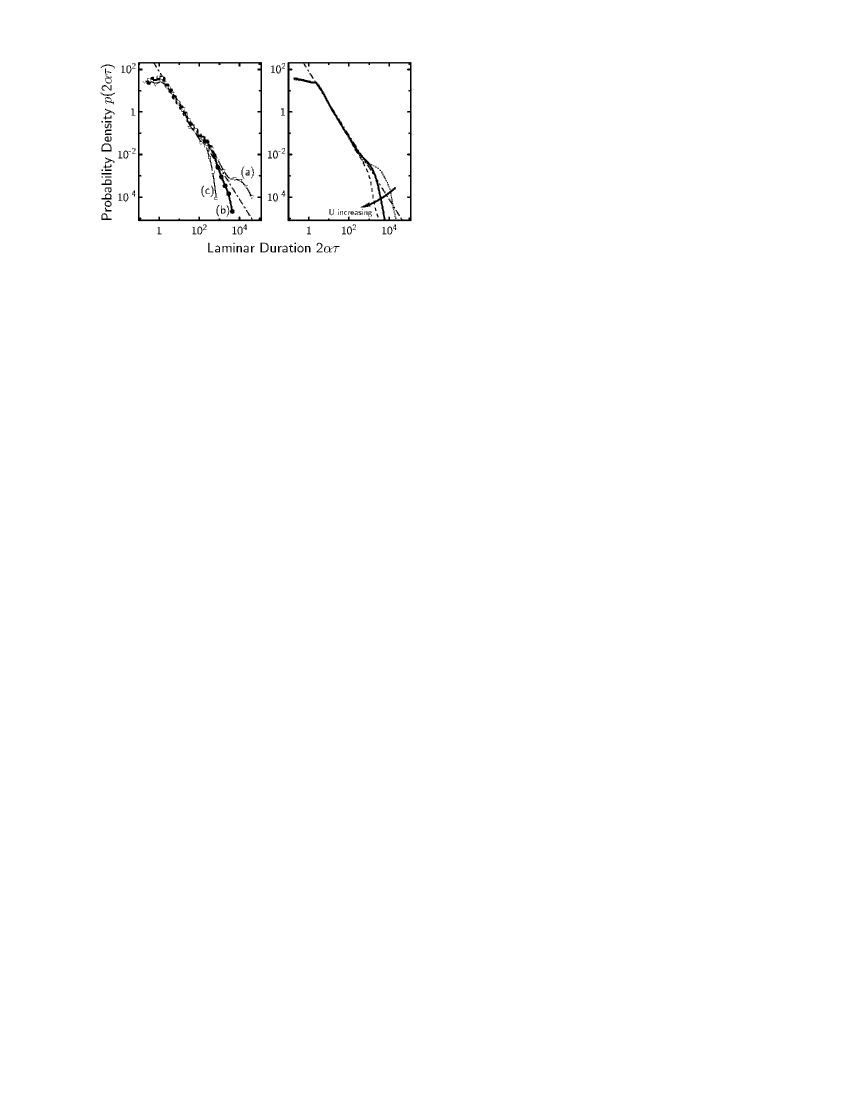
Figure 12: Normalized distribution $p(2\alpha\tau)$ of durations $\tau$ of laminar phases from experimental (left) and simulated (right) trajectories, voltages as in Figs. 11(a-c). Here the trajectories were recorded in 12 bit resolution with a 1 ms sampling rate. The time axis was scaled with the jump rate $\alpha=2\nu$. The threshold $A_{\text{on}}$ is set to 0.05 V. The $\tau^{-3/2}$ power law holds over several decades, best agreement is found at $\text{U}=\text{U}_{\text{c}}^{\text{exp}}$ which we assign to $\lambda=0$.

The statistics of experimental and simulated trajectories can be compared on a quantitative level. In the experiment, the distribution of laminar phases is calculated by introducing an arbitrary threshold intensity $A_{\text{on}}$, and the durations of periods where the intensity curve stays completely below that threshold are determined. A threshold $A_{\text{on}}=0.05$ V has been chosen here, it corresponds to the geometrical average of lower and upper bound of the photo sensor signal. As expected in on-off intermittency, the choice of the actual threshold value is not critical. Fig. 12 (left) depicts the distribution of the laminar phase durations extracted from trajectories for DMP excitation with three different voltages, the same values as in Fig. 11. The time axis is scaled with the jump rate $\alpha$ of the DMP. These distributions were extracted from 4200 sec runs of the experiment, each trajectory has been recorded with a sampling rate of 1000 s^-1 (with the fast AD converter), so that a range of 6 orders of magnitude in $\tau$ is resolved. The dash-dot line indicates a $\tau^{-3/2}$ dependence, which is predicted theoretically exactly at the sample stability threshold, $\lambda=0$, when no additive noise is present. In the short time range, for $2\nu\tau<1$, the curve deviates from this predicted fundamental dependence, because one approaches the time scale of the driving DMP process and specific details of the driving process become important. In the long time limit of the curve, the power law behaviour of the experimental trajectories breaks down mainly because of the lower boundary (additive noise level) for the system variables. For long periods at least one of the variables ($q,\varphi$) reaches a (thermal) noise level which prevents excursions of the system variables to values much below $A_{\text{on}}$, trajectories are practically reflected there. This lead to faster injections of the next burst above $A_{\text{on}}$, and thus to a lower probability of long duration periods. The flat shoulder indicated in Fig. 12 is the outcome of this effect Platt .

Figure 12 (right) shows the results of the corresponding simulations. Limits to the system parameters were set as given in Eq. (13). The voltages used in the simulation are U${}_{\text{c}}^{\text{th}}$=14.2 V (corresponding to the critical value $\lambda=0$), and U${}_{\text{c}}^{\text{th}}\pm$0.7 V chosen in the vicinity of this threshold. The critical voltage in the simulated curves is derived from the analytically calculated Lyapunov exponent Behn98 . It is in perfect agreement with the numerical simulation of the trajectories in absence of upper and lower limits. In the experiment, it has been proposed earlier that a reasonable definition of the critical voltage can be found when the statistical distribution of the laminar phases duration is analyzed. Thus we assume that the experimental critical driving voltage U${}_{\text{c}}^{\text{exp}}$ is reached when the distribution of laminar phases durations is most adapted to a $\tau^{-3/2}$ dependence John . Knowledge of the relation (6) between director deflection amplitudes and scattering intensities is not necessary for the determination of the distribution of laminar phases. On the other hand, the laminar phase distribution is not the most sensitive criterion for the determination of the sample stability threshold as will be shown in the next section.

V.5 Distribution of Pattern Amplitudes

Another fundamental prediction for the statistics of on-off intermittent processes is the distribution of amplitudes in the trajectory. It has been shown Fuji85a ; Fuji85b ; Fujisaka00 ; Nakao that the distribution of the amplitudes of the intermittent variable $\tilde{A}$ should follow a power law

$$p(\tilde{A})\propto\tilde{A}^{-1+\eta}$$ (14)

in the vicinity of the threshold $\lambda=0$. The parameter $\eta\propto\lambda$ vanishes at the threshold of the instability.

A statistical analysis of the recorded trajectories requires knowledge of the quantitative relation (6) between the measured scattering intensity $A$ and the amplitude of the pattern $\varphi$. One can easily show that a similar power law as for the amplitude distributions of the intermittent variable $\varphi$ holds also for quantities $A(\varphi)$ that depend on the $m$th power of $\varphi$. When $p(\varphi)\propto\varphi^{-1+\eta}$ and $A\propto\varphi^{m}$ then

$$p(A)\propto A^{-1+\eta/m}.$$ (15)

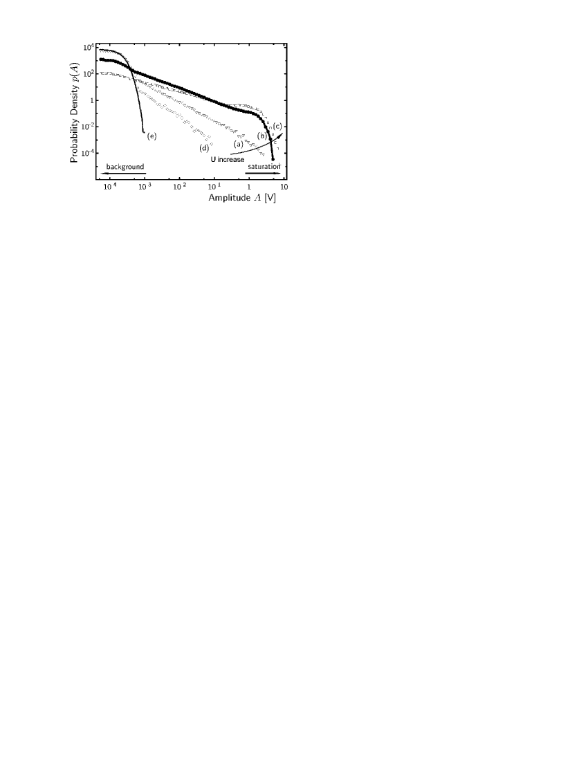
Figure 13: Distribution density of the burst amplitudes $A(t)$ measured over 4200 sec for same DMP voltages as in Figs. 11(a)-(c). (d) for U=11.8 V (large negative $\lambda$ and (e) background at zero excitation voltage. In their middle parts, the distributions fit to a power laws $A^{-1+\eta}$ . From the curve with slope -1 we find the experimental voltage corresponding to $\lambda=0$ .

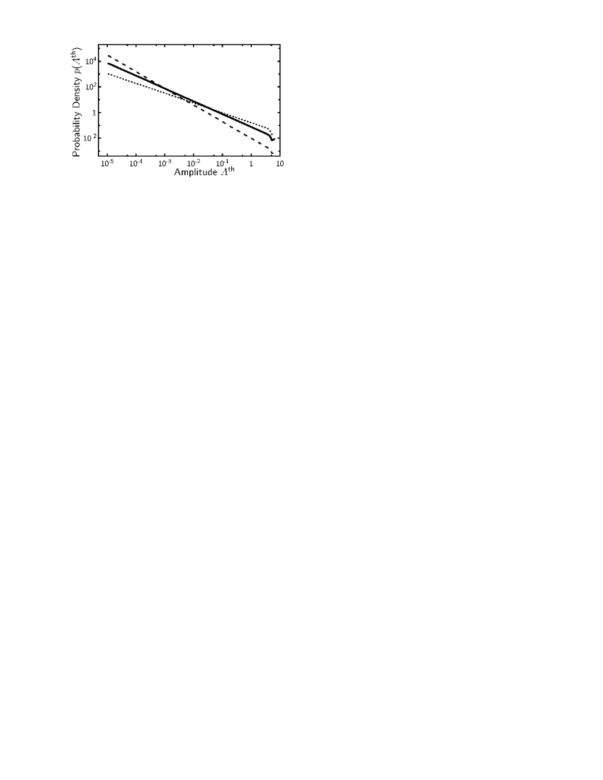
Figure 14: Amplitude distribution densities $p(A^{\text{th}})$ of the simulated trajectories. The power law holds in the complete dynamical range, the fixed boundaries (Eq. (13)) generate abrupt edges in the support of $p(A^{\text{th}})$. The critical voltage U${}_{\text{c}}^{\text{th}}=14.2$ V deviates somewhat from the experimental value. The graphs represent U=14.2 V (solid), 14.9 V (dotted) and 13.5 V (dashed).

The hyperbolic dependence at the threshold $\lambda=0$ is preserved. Our observable $A(t)$, the scattered intensity in the $2$nd order reflex, is related to the director deflection amplitude in first approximation by Eq. (5), and this relation provides another opportunity to determine the critical voltage U${}_{\text{c}}$. Fig. 13 shows the distribution of scattering amplitudes $A(t)$ for zero driving voltage and four representative voltages in the vicinity of the stochastic threshold U${}_{\text{c}}$. A power law can be fitted to the middle part of all these distributions. For low scattering amplitudes, the curve deviates from the fit because of the superimposed background scattering. For large amplitudes, the power law breaks down because of the saturation of the system variables and because the optical characteristics, Eq. (5), is not valid for large director deflections. In the numerically simulated trajectories, Fig. 14, where hard boundaries, cf. Eq. (13) have been used, these effects are condensed in the edges of $p(A)$. $A^{\text{th}}$ is computed from $\varphi$ by means of Eq. (6).

In Fig. 13(b), the amplitude for U=12.9 V is closest to the exponent -1 in the power law, therefore we assign this voltage to the experimental threshold voltage U${}_{\text{c}}^{\text{exp}}$. This value is in good coincidence with the critical voltage found from the best fit of the laminar phase distributions to a $\tau^{-3/2}$ law. Both statistical definitions of the experimental threshold voltage agree consistently, and the numerical simulations confirm the equivalence of the thresholds determined from the distributions of amplitudes and laminar phase durations.

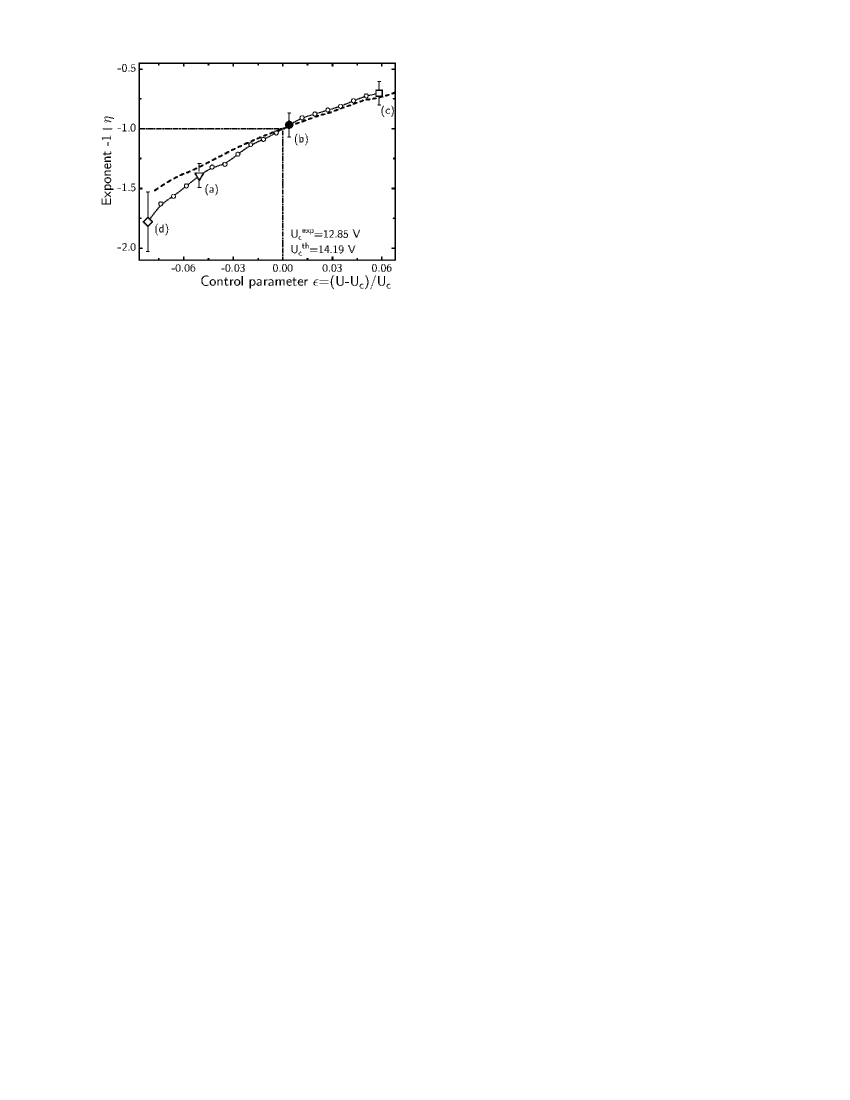
Figure 15: Voltage dependence of the exponent $-1+\eta$ ($\circ$ experiment, - - - simulation). The empirical error bars illustrate the uncertainty of the fit and variations between individual runs of the measurements. For $\epsilon<0$, burst appear infrequently and the statistic is rather poor. A scattering efficiency according to Eq. (6) has been used to relate measured optical data to the simulations ($\tilde{A}\propto|\varphi|\propto A^{1/4}$) and assumed the dash-dotted line the Lyapunov exponent is zero and we correspond this voltage to $\epsilon$=0. Bigger symbols indicate the applied voltages depict in Fig. 13.

At voltages near the threshold, the power law still holds and the exponents $-1+\eta$ can extracted. Typical amplitude distributions are depicted in Figs. 13(c,d). The exponents extracted from experimental data as well as from simulated trajectories are shown in Fig. 15. In accordance with the natural scales of the system, the axis was normalized with the critical voltage to obtain a control parameter $\epsilon$. The optical relation (6) has been applied to retrieve pattern amplitudes $\tilde{A}$ which can be compared to the simulation from experimental scattering intensities $A$. The good agreement in the slopes of the $\eta(\epsilon)$ curves at $\epsilon\geq 0$ justifies the application of the optical relation Eq. (6).

V.6 Power Spectral Density

Finally, we discuss the power spectrum of the intermittent process. The main general theoretical prediction for the power spectral density (PSD) for $\lambda=0$ is a square root frequency dependence miyazaki ; Venkataramani96 ; venka2 ; Fujisaka00 in a certain frequency range. If any quantity with a power law dependence on the intermittent variable is observed, this prediction is equally valid Venkataramani96 . The PSD predicted for a process driven with multiplicative noise is qualitatively different from a process where noise couples additively to the system variables.

In the range of very small frequencies, a constant PSD is expected because any time correlation in the system variables is destroyed by additive noise and the limited dynamical range of ($q,\psi$). In the high frequency tail, a $\text{PSD}\propto\omega^{-2}$ dependence is expected, similar to that of a simple stochastic process with exponentially decaying autocorrelation function. The relation for the high frequency limit $\omega\rightarrow\infty$ can be obtained analytically (from Eq. (50) in Venkataramani96 )

$$\text{PSD}\propto\begin{cases}\text{const}&\text{if $\omega<\omega_{1}$},\\ \omega^{-1/2}&\text{if $\omega_{1}<\omega<\omega_{2}$},\\ \omega^{2}&\text{if $\omega>\omega_{2}$}.\end{cases}$$ (16)

The crossover frequencies $\omega_{1}$, $\omega_{2}$ where the asymptotic exponent changes depend upon the Lyapunov exponent and specific properties of the additive and multiplicative noise.

Fig. 16 displays the PSD of experimentally recorded trajectories $A(t)$ for three voltages (same as in Fig. 12). It was obtained from Fourier transformation of 4.2$\times 10^{6}$ data points of the optical trajectories in an interval of 4200 s. In the logarithmic plot, the curves have been smoothed by averaging the spectral energy over intervals $\Delta\omega$ proportional to $\omega$.

At the threshold voltage $\text{U}_{\text{c}}^{\text{exp}}$ (b), the $\omega^{-1/2}$ and $\omega^{-2}$ regions are well separated, and the existence of a constant PSD in the low frequency wing seems to be indicated. In the high frequency wing, influences of the mean frequency of the driving process, $\nu=80$ Hz, are observable.

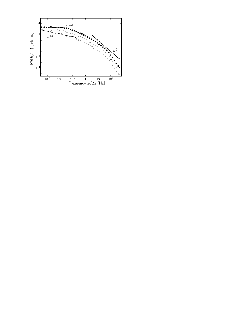
Figure 17: Simulated power spectrum at U${}^{\text{th}}_{\text{c}}$ with different lower bounds ( $\psi_{\min}=5\times 10^{-3}$  ($\bullet$), $10^{-10}$  ($\triangle$), $10^{-100}$  ($\circ$)), upper limit $\psi_{\max}=0.5$. The theoretical exponent -1/2 is found only for unrealistically low background.

The PSD obtained from the numerical simulation (see Fig. 17) are not in agreement with the experiment, in particula the square root dependence is not reproduced. Only when the dynamical range is chosen unrealistically large, we obtain a PSD $\propto\omega^{-1/2}$. The choice of a realistic lower bound (Eq. (13)), i.e. additive noise with reasonable amplitude, destroys any long time correlations. Therefore, a simulation of the PSD with similar parameters as in Figs. 14 yields a pronounced constant low-frequency region.

VI Summary

On-off intermittency in stochastically driven electroconvection of nematic liquid crystals in the conductive regime has been investigated experimentally and by numerical simulations. Results have been presented for excitation with the dichotomous Markov process, but the resulting fundamental statistical behaviour is qualitatively similar for many other types of stochastic excitations.

Laser scattering has been used to determine the wavelengths and time resolved pattern amplitudes. It has been shown experimentally, and confirmed in the simulation of the electro-hydrodynamic equations that under stochastic excitation the pattern selects its wavelength within a narrow band, therefore the intensity of scattered laser light at a fixed scattering angle can used to characterize the temporal behavior of the pattern amplitude. The resulting trajectories have been analyzed quantitatively and their statistical properties have been extracted.

The statistical analysis confirms that the distribution density of laminar phase durations $\tau$ is in full agreement with theoretical predictions. In particular, the $\tau^{-3/2}$ power law describes the statistics of laminar phase durations at the stability threshold in the conduction regime over four decades in $\tau$.

The distribution density of pattern amplitudes $A$ in the vicinity of the instability threshold is also in quantitative agreement with the predicted power law. Deviations are found in the experiment in the limits of low and high pattern amplitudes where additive noise (small A) and nonlinearities in the dynamic equations (large A) influence the dynamical behaviour of the system variables. With increasing voltage the exponent $-1+\eta$ increases. Theory predicts a relation $\eta\propto\lambda$ for on-off intermittence, which allows us to define a critical voltage $\text{U}_{\text{c}}^{\text{exp}}$ from the slopes of the amplitude distribution functions. The critical voltage obtained with this method agrees with the value derived from the analysis of the laminar phase durations, i.e. the two definitions characterize consistently the experimental system as well as the numerically simulations. This provides, irrespective of the fact that the Lyapunov exponent is not directly accessible in the experiment, a quantitative criterion for the stability threshold $\text{U}_{\text{c}}^{\text{exp}}$ of stochastically driven EHC patterns. From a practical aspect, the distribution density of the pattern amplitudes is the more sensitive measure for the determination of $\text{U}_{\text{c}}^{\text{exp}}$.

In the simulations of the corresponding model system, trajectories which are characterized by the $\tau^{-3/2}$ and $A^{-1}$ power laws are obtained when the driving parameters are chosen such that the Lyapunov exponent is zero (sample stability threshold Behn98 ). This result coincides with theoretical predictions of the universal behaviour of on-off intermittency Heagy . In the vicinity of the critical voltage the linear dependence of the exponent $-1+\eta$ on $\lambda$ is also in quantitative agreement with the numerical simulation. In the experiment, we cannot relate the exponent of the amplitude distribution to a Lyapunov exponent. However, the functional dependence of $\eta$ on the reduced voltage $\epsilon$ is in satisfactory agreement with the calculated data (see Fig. 15).

We note that although the statistical characterization of experimental and simulated data are in good quantitative agreement, the experimental and calculated threshold voltages and wave numbers can differ on an absolute scale by roughly 10% (see Fig. 2). This is mainly the consequence of the simplified assumptions of director and flow modes in the model, it is not relevant for the description of on-off-intermittent behaviour.

In the power spectrum of the experimental trajectories, a $\omega^{-1/2}$ dependence is indicated in a small frequency range, in agreement with predictions of general theories miyazaki ; Venkataramani96 , in the high frequency tail, the PSD adopts an $\omega^{-2}$ behavior (Fig. 16). In the numerical simulations with boundaries to the system variables, (Fig. 17) we did not find the $\omega^{-1/2}$ dependence, it is reproduced only when boundaries of the trajectory are disregarded and a simulation with quasi unlimited dynamical amplitude range is performed. This discrepancy leads us to the conclusion that the PSD is particularly sensitive to additive noise and the full nonlinear dynamical equations. The appearance of the $\omega^{-1/2}$ range in the experimental data in apparent agreement with general predictions should therefore not be overestimated.

We note that although the investigated experimental system represents a spatially extended dissipative system, it has been shown in this study that its fundamental statistical properties can be reproduced in simulations of a 2$\times$2 evolution matrix model with global pattern amplitude, thus neglecting spatial details of the pattern. In the case of a global driving parameter, the spatial phase does not play a role as long as other noise sources are excluded. Additive noise, however, may introduce phase drifts in the system Fuji01 ; Fujipriv and is responsible for a complex spatio-temporal characteristics. A detailed spatio-temporal description of the system represents an ongoing interesting task.

Thanks is due to Hirokazu Fujisaka for stimulating discussions.

The authors acknowledge financial support from the Deutsche Forschungsgemeinschaft (Grant Be 1417/4) and SFB 294.

Parameter		Simulation input		Exp. value
$n_{\text{o}}$		1.	4935	1.	4935
$n_{\text{e}}$		1.	6315	1.	6315
$\varepsilon_{\scriptscriptstyle\parallel}$		6.	24	6.	24
$\varepsilon_{\scriptscriptstyle\perp}$		6.	67	6.	67
$\sigma_{\scriptscriptstyle\parallel}$	$[\mbox{s}^{-1}]$	90.	0	117.	0
$\sigma_{\scriptscriptstyle\perp}$	$[\mbox{s}^{-1}]$	60.	0	90.	0
$\alpha_{1}$	$[\mbox{g\thinspace cm}^{-1}\mbox{s}^{-1}]$	0.	1
$\gamma_{1}$	$[\mbox{g\thinspace cm}^{-1}\mbox{s}^{-1}]$	3.	3	3.	6
$\gamma_{2}$	$[\mbox{g\thinspace cm}^{-1}\mbox{s}^{-1}]$	-3.	3
$\beta$	$[\mbox{g\thinspace cm}^{-1}\mbox{s}^{-1}]$
$\eta_{1}$	$[\mbox{g\thinspace cm}^{-1}\mbox{s}^{-1}]$	3.	62
$\eta_{2}$	$[\mbox{g\thinspace cm}^{-1}\mbox{s}^{-1}]$	1.	0
$K_{11}$	$[\mbox{g\thinspace cm\thinspace s}^{-2}]$	14.	9 $\times 10^{-7}$	14.	9$\times 10^{-7}$
$K_{33}$	$[\mbox{g\thinspace cm\thinspace s}^{-2}]$	13.	76 $\times 10^{-7}$	13.	76$\times 10^{-7}$

Table 1: Material parameters (cgs) used in the simulations. The parameter set for the simulations of stochastic trajectories is taken from the fit of threshold voltage and wave number characteristics for periodic AC driving, see also Fig. 2. Experimentally data for Mischung 5 taken from amm99 ; MGRS

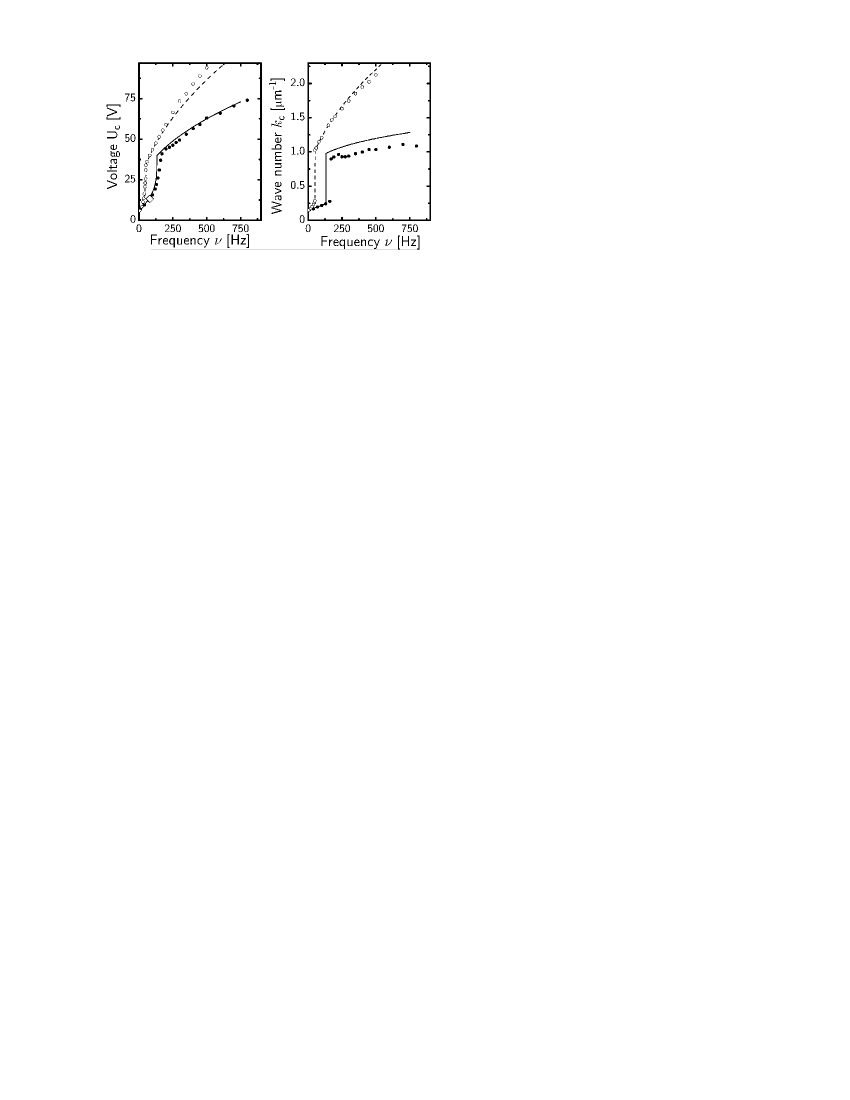
Figure 2: Threshold voltages and wave numbers for driving with periodic and stochastic (DMP) square waves of (mean) frequency $\nu$. Periodic excitation: experiment ($\circ$), theory (- - -), stochastic excitation: experiment ($\bullet$), theory (-​-​-​-​-). The method for the experimental determination of stochastic thresholds is explained in the text. The symbol $\diamond$ indicates the frequency, where the stochastic measurements presented below have been performed.

Figure 16: Power spectral density of trajectories (a)-(c) in Fig. 12. AD-converter with 1 ms sample time and 12 bit resolution was used. General predictions for the PSD in on-off intermittency are an exponent zero for very low frequencies, (-1/2) for medium frequencies and (-2) for high frequencies, see Eq. (16). Near the critical voltage U${}_{\text{c}}^{\text{exp}}$, the experimental data indicate such a behaviour. The curve has been smoothed by averaging the density over intervals proportional to frequency.

References

- (1) Y. Pomeau and P. Manneville, Phys. Lett. A 75, 1 (1979).
- (2) H. G. Schuster, ’Deterministic Chaos’, Ch. 4 (VCH, Weinheim, 1987).
- (3) H. Fujisaka and T. Yamada, Progr. Theor. Phys. 74, 918 (1985).
- (4) H. Fujisaka and T. Yamada, Progr. Theor. Phys. 75, 1087 (1985).
- (5) T. Yamada and H. Fujisaka, Progr. Theor. Phys. 76, 582 (1986).
- (6) N. Platt, E. A. Spiegel, and C. Tresser, Phys. Rev. Lett. 70, 279 (1993).
- (7) J. F. Heagy, N. Platt, and S. M. Hammel, Phys. Rev. E 49, 1140 (1994).
- (8) T. Yamada, K. Fukushima, and T. Yazaki, Progr. Theor. Phys. Suppl. 99, 120 (1989).
- (9) D. L. Feng, C. X. Yu, J. L. Xie, and W. X. Ding, Phys. Rev. E 58, 3678 (1998).
- (10) F. Rödelsperger, A. Čenys, and H. Benner, Phys. Rev. Lett. 75, 2594 (1995).
- (11) T. John, R. Stannarius, and U. Behn, Phys. Rev. Lett. 83, 749 (1999).
- (12) H. Fujisaka, S. Matsushita, T. Yamada, and H. Tominaga, Phys. Reports 290, 27 (1997).
- (13) H. L. Yang and E. J. Ding, Phys. Rev. E 50, R3295 (1994).
- (14) Z. Qu, F. Xie, and G. Hu, Phys. Rev. E 53, R1301 (1996).
- (15) F. Xie and G. Hu, Phys. Rev. E 53, 4439 (1996).
- (16) H. L. Yang, Z. Q. Huang, and E. J. Ding, Phys. Rev. E 54, 3531 (1996).
- (17) W. Yang, E. J. Ding, and M. Ding, Phys. Rev. Lett. 76, 1808 (1996).
- (18) N. Platt and S. M. Hammel, Physica A 239, 296 (1997).
- (19) H. Fujisaka, K. Ouchi, H. Hata, B. Masaoka, and S. Miyazaki, Physica D 114, 237 (1998).
- (20) K. Fukushima and T. Yamada, Phys. Lett. A 237, 141 (1998).
- (21) S. Miyazaki and H. Hata, Phys. Rev. E 58, 7172 (1998).
- (22) S. C. Venkataramani, T. A. Antonson, E. Ott, and J. C. Sommerer, Physica D 96, 66 (1996).
- (23) S. C. Venkataramani, T. M. Antonsen, E. Ott, and J. C. Sommerer, Phys. Lett. A 207, 173 (1995).
- (24) O. V. Gerashchenko, S. L. Ginzburg, and M. A. Pustovoit, Europhys. J. B 15, 335 (2000).
- (25) M. Sauer and F. Kaiser, Phys. Rev. E 54, 2468 (1996).
- (26) H. Fujisaka, H. Suetani, and T. Watanabe, Progr. Theor. Phys. Suppl. 139, 70 (2000).
- (27) H. Nakao, Phys. Rev. E 58, 1591 (1998).
- (28) U. Behn, A. Lange, and T. John, Phys. Rev. E 58, 2047 (1998).
- (29) R. Williams, J. Chem. Phys. 39, 384 (1963).
- (30) E. F. Carr, J. Chem. Phys. 38, 1536 (1963).
- (31) W. Helfrich, J. Chem. Phys. 51, 4092 (1969).
- (32) Orsay Liq. Cryst. Group, Phys. Rev. Lett. 26, 1642 (1970).
- (33) E. Dubois-Violette, P. G. de Gennes, and O. Parodi, J. Physique 32, 305 (1971).
- (34) I. W. Smith, Y. Galerne, S. T. Lagerwall, E. Dubois-Violette, and G. Durand, J. Physique Coll. C1, 237 (1975).
- (35) L. Kramer and W. Pesch, Annu. Rev. Fluid Mech. 17, 515 (1995).
- (36) H. R. Brand, S. Kai, and S. Wakabayashi, Phys. Rev. Lett. 54, 555 (1985).
- (37) H. Amm, U. Behn, T. John, and R. Stannarius, Mol. Cryst. Liq. Cryst. 304, 525 (1997).
- (38) S. Kai, T. Kai, M. Takata, and K. Hirakawa, J. Phys. Soc. Jpn. 47, 1379 (1979).
- (39) T. Kawakubo, A. Yanagita, and S. Kabashima, J. Phys. Soc. Jpn. 50, 1451 (1981).
- (40) S. Kai, H. Fukunaga, and H. R. Brand, J. Phys. Soc. Jpn. 56, 3759 (1987).
- (41) S. Kai, H. Fukunaga, and H. R. Brand, J. Stat. Phys. 54, 1133 (1989).
- (42) S. Kai, in Noise in nonlinear dynamical systems, edited by F. Moss and P. V. E. McClintock (Cambridge University Press, Cambridge, 1989), p. 22.
- (43) U. Behn and R. Müller, Phys. Lett. 113A, 85 (1985).
- (44) R. Müller and U. Behn, Z. Phys. B 69, 185 (1987).
- (45) R. Müller and U. Behn, Z. Phys. B 78, 229 (1990).
- (46) A. Lange, R. Müller, and U. Behn, Z. Phys. B 100, 447 (1996).
- (47) H. Amm, M. Grigutsch, and R. Stannarius, Z. Naturforschung A 53a, 117 (1998).
- (48) H. Bohatsch and R. Stannarius, Phys. Rev. E 60, 5591 (1999).
- (49) H. Amm, R. Stannarius, and A. Rossberg, Physica D 126, 171 (1999).
- (50) M. Grigutsch and R. Stannarius, unpublished.
- (51) U. Bisang and G. Ahlers, Phys. Rev. Lett. 80, 3061 (1998).
- (52) U. Bisang and G. Ahlers, Phys. Rev. E 60, 3910 (1999).
- (53) S. Rasenat, G. Hartung, B. L. Winkler, and I. Rehberg, Experiments in Fluids 7, 412 (1989).
- (54) S. S. Y. L. K. Vistin, A. Yu. Kabaenkov, Sov. Phys. - Crystallogr. 26, 70 (1981).
- (55) K. Kondo, A. Fukuda, and E. Kuze, Jpn. J. Appl. Phys. 20, 1779 (1981).
- (56) K. Kondo, A. Fukuda, E. Kuze, and M. Arakawa, Jpn. J. Appl. Phys. 22, 394 (1983).
- (57) I. Rehberg, F. Horner, and G. Hartung, J. Stat. Phys. 64, 1017 (1991).
- (58) J. A. Kosmopoulos and H. M. Zenginoglou, Appl. Optics 26, 1714 (1987).
- (59) A. Joets and R. Ribotta, Opt. Commun. 107, 200 (1994).
- (60) A. Joets and R. Ribotta, J. Physique I 4, 1013 (1994).
- (61) T. O. Carroll, J. Appl. Phys. 43, 767 (1972).
- (62) R. A. Kashnow and J. E. Bigelow, Applied Optics 10, 2302 (1973).
- (63) P. L. Papadopoulos, H. M. Zenginoglou, and J. A. Kosmopoulos, J. Appl. Phys. 86, 3042 (1999).
- (64) M. Bouvier and T. Scharf, Opt. Eng. 39, 2129 (2000).
- (65) H. M. Zenginoglou and J. A. Kosmopoulos, Applied Optics 28, 3516 (1989).
- (66) H. M. Smith, Holographic Recording (Springer, Berlin, 1977).
- (67) I. Rehberg, S. Rasenat, M. de la Torre Juárez, W. Schöpf, F. Hörner, G. Ahlers, and H. R. Brand, Phys. Rev. Lett. 67, 596 (1991).
- (68) R. F. Fox, I. R Gatland, R. Roy, and G. Vemuri, Phys. Rev. A 38, 5938 (1988).
- (69) A. Čenys, A. N. Anagnostopoulos, and G. L. Bleris, Phys. Rev. E 56, 2592 (1997).
- (70) H. Fujisaka, K. Ouchi, and H. Ohara, Phys. Rev. E 64, 036201 (2001).
- (71) H. Fujisaka, priv. information.