Euler–Poincaré Characteristic and
Phase Transition in the Potts Model

Abstract: Recent results concerning the topological properties of random geometrical sets have been successfully applied to the study of the morphology of clusters in percolation theory. This approach provides an alternative way of inspecting the critical behaviour of random systems in statistical mechanics.

For the 2d $q$-states Potts model with $q\leq 6$, intensive and accurate numerics indicates that the average of the Euler characteristic (taken with respect to the Fortuin-Kasteleyn random cluster measure) is an order parameter of the phase transition.

Key words: Cluster Morphology, Euler-Poincaré characteristic, Phase Transition.

1 Introduction

Recently, new insights in the study of the critical properties of clusters in percolation theory have emerged based on ideas coming from mathematical morphology [Se] and integral geometry [Ha, S, Sch]. These mathematical theories provide a set of geometrical and topological measures allowing to quantify the morphological properties of random systems. In particular these tools have been applied to the study of random cluster configurations in percolation theory and statistical physics [MW, O, J, Wa1, M1].

One of these measures is the Euler-Poincaré characteristic $\chi$ which is a well known descriptor of the topological features of geometric patterns. It belongs to the finite set of Minkowski functionals whose origin lies in the mathematical study of convex bodies and integral geometry (see [Ha, S, Sch]). These measures, as we shall explain below, share the following remarkable property: any homogeneous, additive, isometry-invariant and conditionally continuous functional on a compact subset of the Euclidean space $\mathbb{R}^{d}$ can be expressed as a linear combination of the Minkowski functionals. This is the well known Hadwiger’s theorem [Ha] of integral geometry which has a wide scope of applications in mathematical physics due its rather general settings.

The use of these measures in image analysis [Gra], problems of shape recognition [Se], determination of the large scale structures of the universe [Wa2], modelling of porous media [AKPM], microemulsions [HK] and fractal analysis [M2] has been a topic of growing interest recently.

The application of these description tools for the study of random systems in statistical mechanics has already provided interesting results. In [MW, O], the computation of the Euler-Poincaré characteristic $\chi$ for a system of penetrable disks in several models of continuum percolation has led to conjecture new bounds for the critical value of the continuum percolation density. In [MW], an exact calculation of $\chi$ has shown that a close relation exists between the zero of the Euler-Poincaré characteristic and the critical threshold for continuum percolation in dimensions $2$ and $3$.

Of similar interest in the same domain, let us recall that for the problem of bond percolation on regular lattices, Sykes and Essam [SyEs] were able to show, using standard planar duality arguments, that for the case of self-dual matching lattices (e.g. $\mathbb{Z}^{2}$), the mean value of the Euler-Poincaré characteristic changes sign at the critical point (this even led them to announce a proof for the existence of the critical probability of bond percolation on $\mathbb{Z}^{2}$), see also [Gri].

More recently, Wagner [Wa1] was able to compute the Euler-Poincaré characteristic on the set of all plane regular mosaics (the $11$ archimedean lattices) as a function of the site occupancy probability $p\in[0,1]]$ and showed that a close connection exists between the threshold for site percolation on these lattices and the point where the Euler-Poincaré characteristic (expressed as a function of $p$) changes sign.

The aim of this article is to further investigate the role played by this morphological indicator in statistical physics and to present new results concerning its behaviour in the case of the 2-dimensional Potts model. Namely we present here clear evidence, based on Monte Carlo simulations, that for the 2d Potts model, the Euler-Poincaré characteristic is an order parameter of the phase transition. Namely we find that for $q=2,...,4$ it changes sign continuously at the transition point while, for $q=5,6$ it has a first order transition at the critical point. As far as we know, this is the first example of a discontinuous behaviour of this parameter in a physical model.

The paper is organized as follows. In Section 2 we introduce a minimal background concerning Minkowski functionals and the necessary definitions for our model, the numerical results are presented in Section 3 followed by some comments and discussion in Section 4.

2 The model

We first briefly summarize the basic facts from integral geometry and give the definition of the Minkowski functionals including the Euler-Poincaré characteristic, see [Ha, S, Sch] for more complete expositions. We will then show how to compute the Euler-Poincaré characteristic in the case of a random configuration of sites and bonds produced by a Fortuin-Kasteleyn (FK) transformation of the partition function of the Potts model [FK].

Minkowski Functionals

In the most abstract setting, the Minkowski functionals are defined as integrals of curvatures in the framework of the differential geometry of smooth surfaces in compact sub–domains of the Euclidean space $\mathop{\rm I\!R}^{d}$ [Ha].

Another way to introduce these measures is as follows. First define the Euler-Poincaré characteristic $\chi$ as an additive functional on subsets of $\mathop{\rm I\!R}^{d}$ such that for $A,B\subset\mathop{\rm I\!R}^{d}$ (see example in Fig. 1)

$$\chi(A\cup B)=\chi(A)+\chi(B)-\chi(A\cap B)$$ (2.1)

with

$$\chi(A)=\begin{cases}1,\;\mbox{if}\;A\neq\emptyset\mbox{, A convex}\\ 0,\;A=\emptyset.\end{cases}$$

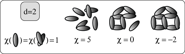
Figure 1: Examples of calculation of the Euler-Poincaré characteristic in dimension $d=2$ for some combinations of convex subsets of $\mathop{\rm I\!R}^{2}$.

The set of Minkowski functionals is then defined by (see e.g. [Gra, MW])

$$W_{\alpha}(A) = \int\chi(A\cup E_{\alpha})\,d\mu(E_{a}),\;\;\;\alpha=0,...,d-1$$ (2.2)

$$W_{d}(A) = \omega_{d}\,\chi(A):\;\;\;\omega_{d}=\pi^{d/2}/\Gamma(1+d/2)$$ (2.3)

where $E_{\alpha}$ is an $\alpha$-dimensional plane in $\mathop{\rm I\!R}^{d}$, $d\mu(E_{a})$ its density normalized such that, for the $d$-dimensional ball $B_{d}(r)$ with radius $r$, $W_{\alpha}(B_{d}(r))=\omega_{d}\,r^{d-\alpha}$ and $\omega_{d}$ is the volume of the unit ball in $\mathop{\rm I\!R}^{d}$.

Obviously, additivity of the Minkowski functionals is inherited from (2.1), furthermore they are conveniently normalized through

$$M_{\alpha}(A)=\frac{\omega_{d-\alpha}}{\omega_{d}\,\omega_{\alpha}}W_{\alpha}(A)$$

The computation of these normalized functionals in dimensions $1,2,3$ in term of the usual geometric measures (length, area, volume,…) is given in Table 1.

$d$	$\;\;\;M_{0}\;\;\;$	$\;\;\;M_{1}\;\;\;$	$M_{2}$	$M_{3}$
1	$L$	$\chi_{1}/2$	$\cdots$	$\cdots$
2	$S$	${\cal C}$	$\chi_{2}/\pi$	$\cdots$
3	$V$	$S$	$H/2\pi^{2}$	$3\chi_{3}/4\pi$

Table 1: Values of the normalized Minkowski functionals for $d$-dimensional subsets of $\mathop{\rm I\!R}^{d},d=1,2,3$ in terms of geometric measures, $L$: length, $S$: area, $V$: volume, ${\cal C}$: circumference, $H$: integral mean curvature, $\chi_{d}$: Euler-Poincaré characteristic.

Hadwiger’s completeness theorem asserts that, under not too restrictive and furthermore physically reasonable assumptions, namely: additivity, motion invariance (under translations and rotations) and conditional continuity (which states that any convex body can be smoothly approximated by convex polyhedra), any functional ${\cal M}$ decomposes as a linear combination of the finite set of Minkowski functionals

$${\cal M(A)}=\sum_{\nu=0}^{d}c_{\nu}\,M_{\nu}(A)$$

where the $c_{\nu}$ are real coefficients.

This theorem has very important practical consequences, we refer to [Ha, S, Gra], we shall only mention the principal kinematic formula (see [S, M1])

$$\int_{\cal G}M_{\alpha}(A\cup gB)dg=\sum_{\beta=0}^{\alpha}{\binom{\alpha}{\beta}}M_{\alpha-\beta}(B)M_{\beta}(A),\;\alpha=0,...,d$$

where integration is over the group of motions (i.e. rotations and translations, $g=(r,\Theta)$). This formula is very useful to calculate mean values of Minkowski functionals for random distributions of objects. For instance, it can be applied to the computation of the excluded volume of convex bodies (leading, in case of spherical objects, to Steiner’s formula), which has been used to estimate the critical thresholds in continuum percolation theory [Ba, PS].

In the following, we will be mainly interested in the evaluation of the Euler-Poincaré characteristic for random bond configurations on regular lattices $\Lambda\subset{\mathbb{Z}}^{d}$ which, as we shall see, is equivalent to compute Euler formula for planar graphs made of ${\cal S}$ sites (or nodes), ${\cal B}$ bonds (or links) and ${\cal P}$ plaquettes (or faces) [Ag, Be], i.e.

$$\chi={\cal S}-{\cal B}+{\cal P}$$

It is indeed one of the topics of algebraic topology to show that the above general definitions of Minkowski functionals extend to cell complexes (see Appendix) to which random bond configurations on regular lattices belong.

Because of the growing interest in the use of these morphological measures, we thought that it was important to recall briefly their definitions and main properties.

Potts Model

The partition function for the $q$-states Potts model on $\Lambda\subset\mathbb{Z}^{d}$ at inverse temperature $\beta$ reads

$$Z_{\beta,q}^{\rm Potts}(\Lambda)=\sum_{\boldsymbol{\sigma}}\exp\bigg{\{}\beta\sum_{<i,j>\subset\Lambda}\delta(\sigma_{i},\sigma_{j})\bigg{\}}$$ (2.4)

where the first sum runs over all configurations $\boldsymbol{\sigma}\subset\{1,\dots,q\}^{|\Lambda|}$, the second one is over each nearest neighbour pair of Potts spins on $\Lambda$ and $\delta$ is the Kronecker symbol. We remind that, whenever $q$ is large enough, in any dimension $d\geq 2$, this model exhibits a unique (inverse) temperature $\beta_{c}$ where the mean energy is discontinuous (see [K, LMR, KLMR]). In dimension $d=2$ for $q\geq 5$ this is an exact result [Bax] and it is expected to be true, in $d=3$, for $q\geq 3$ [Wu].

After performing the (FK) transformation [FK], the partition function (2.4) leads to the following random cluster representation

$$Z_{\beta,q}^{\rm FK}(\Lambda)=\sum_{X}(e^{\beta}-1)^{N^{1}(X)}q^{N_{\Lambda}(X)}$$ (2.5)

Here the summation is over all graphs $X$ which can be drawn inside the domain $\Lambda$, $N^{1}(X)$ is the number of bonds of the configuration $X$ and $N_{\Lambda}(X)$ is the number of connected components of $X$ (including isolated sites). We will call $N^{0}(X)$ the number of sites which are endpoints of a bond in $X$ and $N^{2}(X)$ the number of plaquettes of the configuration $X$, i.e. the set of cells in $\Lambda$ having 4 occupied bonds on its boundary (see Fig. 2).

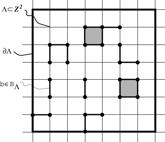
Figure 2: A bond configuration $X\subset B_{\Lambda}$ with 25 sites, 19 bonds and 2 plaquettes.

In this framework, the Euler-Poincaré formula [Ag] leads to the following definition of the Euler-Poincaré characteristic

$$\chi(X)=N^{0}(X)-N^{1}(X)+N^{2}(X)$$ (2.6)

This expression will allow us to compute the mean value of the Euler-Poincaré characteristic with respect to the FK measure.

In algebraic topology, one is interested in classifying geometric objects (or spaces) up to some transformations acting on these spaces (homeomorphisms) by means of simple invariant quantities. It turns out that this program can be achieved and such invariants of a space are the homology groups of these spaces. In this framework, the Euler-Poincaré characteristic (as the other Minkowski functionals) can be expressed in terms of these invariants and lead to a definition for $\chi$ equivalent to the one given by (2.6) (see Appendix).

3 Numerical Results

We have performed Monte Carlo simulations of the 2-dimensional $q$-state Potts model for $q$ ranging from $2$ to $6$. We have always simulated the models near the critical temperature, whose value can be exactly determined through the well known formula: $\beta_{c}(q)=J/kT_{c}(q)=\log(1+\sqrt{q})$. In order to extract a value of the Euler characteristic $\chi$ as close as possible to the value at the infinite volume limit, we have taken rather large lattices: for the three models with a continuous transition ($q=2,3,4$) we arrived at lattice sizes up to $2000^{2}$. The algorithm we used is the Wolff cluster update [Wo]. The identification of FK cluster configurations has been performed via the Hoshen–Kopelman algorithm [Ho]; we always considered free boundary conditions for the cluster labeling.

The Wolff algorithm is the less efficient the bigger the number $q$ of states. Particularly dramatic is what happens when one passes from the 2-state (Ising) to the 3-state model: in the former case, on the $2000^{2}$ lattice it is enough to perform few updates ($5-10$) to get uncorrelated configurations for the cluster variables, in the latter one needs about 1000 updates! Because of that, the simulations for $q=3,4$ on the $2000^{2}$ lattice were very slow, and the relative data could not reach a high statistics. Nevertheless, as we will see, we can get useful indications out of them.

If $\chi$ changes sign at the threshold, on a finite lattice the values measured at each iteration would be distributed around zero, provided the lattice is large enough. Therefore one would see both positive and negative values. For this reason, it is helpful to look at the distribution of $\chi$. In the following we present separately the results for $q=2,3,4$ and $q=5,6$.

3.1 Results for the models with a continuous phase transition

The first case we consider here is the Ising model. Fig. 3 shows the $\chi$ distribution for three different lattice sizes: $500^{2}$, $1000^{2}$ and $2000^{2}$. In each case we have taken 20000 measurements. The peak of the distribution shifts towards $\chi=0$ the larger the lattice. The average values of $\chi$ are: $\chi(500^{2})=0.00101(2)$, $\chi(1000^{2})=0.00053(2)$, $\chi(2000^{2})=0.00024(1)$. We notice that the averages are quite small and decrease sensibly if we go to larger sizes, reducing themselves to about the half when we pass from a lattice to the next one. This approximate linear scaling of $\chi$ with the lattice side suggests that the Euler characteristic at the infinite volume limit indeed vanishes.

Let us now examine the case $q=3$. In Fig. 4 we again plot the $\chi$ distribution for the same three lattice sizes we have considered for the Ising model.

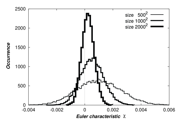
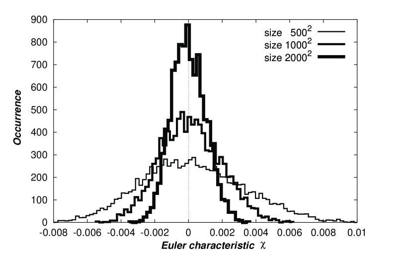
Figure 3: Distribution of $\chi$ for the FK cluster configurations of the 2d Ising model at the critical point.

Figure 4: Distribution of $\chi$ for the FK configurations of the 2d, 3-state Potts model at the critical point.

Since we collected a different number of measurements for the different lattices, for a real comparison of the distributions we needed to renormalize the total number of measurements on each lattice to the same value: we decided to renormalize all data sets to the number of measurements on the $500^{2}$ lattice (10000). The distributions are broader than the Ising ones but they appear almost exactly centered at $\chi=0$. The average values are in fact much smaller than before: $\chi(500^{2})=0.00024(4)$, $\chi(1000^{2})=0.00012(3)$, $\chi(2000^{2})$ is zero within errors. We then deduce that also for $q=3$ $\chi=0$ at the critical point.

To complete our analysis we studied the case $q=4$. In Fig. 5 we present a comparison of the $\chi$ distributions for two lattice sizes, $800^{2}$ and $2000^{2}$.

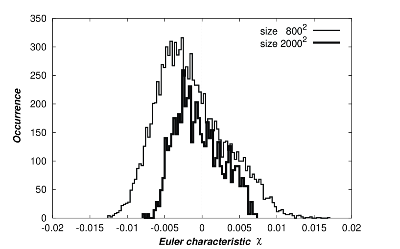
Figure 5: Distribution of $\chi$ for the FK cluster configurations of the 2d, 4-state Potts model at the critical point.

There is a clear shift of the center of the distribution towards zero when one goes from the smaller to the larger lattice. The average values of the Euler characteristic in the two cases are $\chi(800^{2})=-0.00145(8)$ and $\chi(2000^{2})=-0.0006(2)$. Also here there is no apparent convergence to some value, even if the lattices are rather large: $|<\chi>|$ reduces itself to less than its half by changing the lattice size. From all this we also deduce that the Euler characteristic of the FK clusters of the 2-dimensional 4-state Potts model vanishes at criticality.

3.2 Results for the models with a first order phase transition

For $q>4$ the 2d $q$-state Potts model undergoes a first order phase transition, i.e. the thermal variables vary discontinuously at the critical threshold. The magnetization, for instance, makes a jump, varying from zero to a non-zero value. Because of that, we expect that the cluster configurations change abruptly at the critical point, and that the cluster variables exhibit as well discontinuities. In particular, the Euler characteristic may jump from a value to another.

We analyze here the 5- and 6-state Potts models. In both cases we have performed simulations on a $300^{2}$ lattice. In Figs. 6 and 7 we compare the distribution histograms of the magnetization $M$ and the Euler characteristic $\chi$ at three different temperatures: above, near and below $T_{c}$. We define the magnetization by taking the excess of sites in the majority spin state with respect to the value $1/q$ in the paramagnetic phase, when all spin states are equally distributed. Therefore we always measure $M>0$. Looking at the magnetization histograms one clearly sees the spontaneous symmetry breaking by reducing the temperature. The characteristic double peak structure of $M$ around $T_{c}$ indicates that the transition is first order, as it is known. The corresponding histograms of the Euler characteristic show a perfectly analogous pattern. As we expected, the two coexisting FK-phases at $T_{c}$ are characterized by two different values of the Euler characteristic (double peak in the figures). The ordered phase is made of bonds between Potts spins of the same color at $T_{c}$. We then deduce that $\chi$, like $M$, varies discontinuously at the threshold. The result is valid for the 5-state and the 6-state Potts model, so it is likely to be valid also for $q>6$, when the discontinuity of $M$ at the threshold is sharper. Looking at both figures we remark that the centers of the peaks of $\chi$ look approximately symmetric with respect to zero. If this symmetry exists, it would be an interesting feature, and at the moment we have no arguments to justify it. In order to determine with some accuracy the values of $\chi$ in the two coexisting phases we would need to increase considerably the size of the lattice, but the required computer time would increase dramatically for the reasons we explained at the beginning of this section.

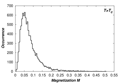
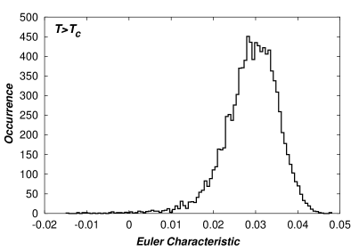
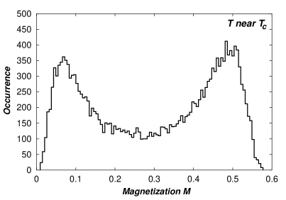
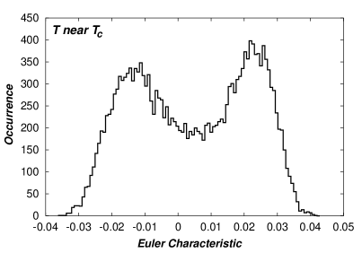
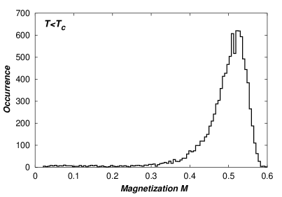
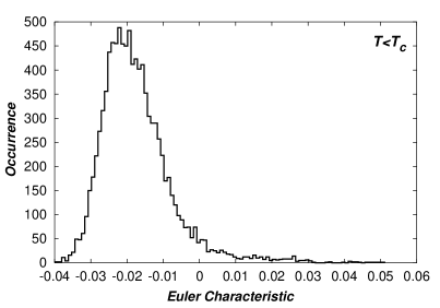
Figure 6: Distribution histograms of the magnetization $M$ and the Euler characteristic $\chi$ for the 2-dimensional 5-state Potts model at three different temperatures. The lattice size is $300^{2}$. The behaviour of $\chi$ is driven by $M$.

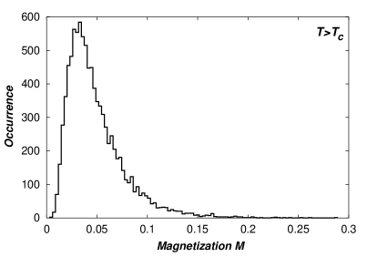
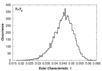
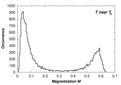
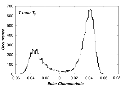
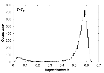
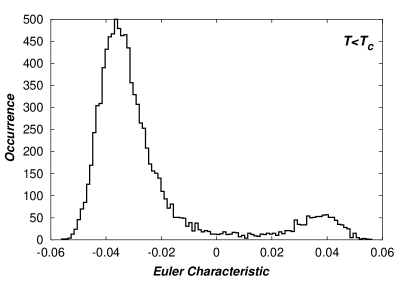
Figure 7: Distribution histograms of the magnetization $M$ and the Euler characteristic $\chi$ for the 2-dimensional 6-state Potts model at three different temperatures. The lattice size is $300^{2}$. The behaviour of $\chi$ is driven by $M$.

4 Conclusions

This work clearly indicates and confirms that the Euler-Poincaré characteristic is indeed an important indicator of a phase transition, playing the role of an order parameter for the $2$-$d$ Potts model, to the extend of the cases ($q=2,...,6$) studied here. For this model, it reveals that the topology of cluster configurations has a deep meaning concerning criticality.

The fact that $\chi$ changes sign at $T_{c}$ can be understood in the following way. Let us consider the 2D Ising model: from $T_{c}$ up to $T=\infty$ the system is in its disordered phase and the only excitations one can get in the FK-bond representation are made of isolated bonds (the probability to see any plaquette vanishes exponentially). Applying (6.1) (see Appendix), one sees that $\chi$ behaves like $\beta^{0}(X)$ times a term of the order of the volume of the system. However, from $T_{c}$ down to $T=0$, the system is in its ordered phase and the corresponding FK-configuration is (with high probability) made of $O(1)$ connected bond components. Missing bonds constitute the excitations and their number scales with the volume of the system so, using again (6.1), one gets that $\chi$ behaves like $-\beta^{1}(X)$ times a term of the order of the volume of the system. This explains in the case of the Ising model the change of sign of $\chi$ at $T_{c}$.

Other spin systems have to be investigated in order to see whether this property of the Euler-Poincaré characteristic is shared by models with continuous symmetries such as the $X$-$Y$-model or the Widom-Rowlinson model.

Another important question concerns the critical behaviour in gauge models. For example a similar study could provide some insights concerning the deconfining transition in SU(N) gauge theory. Indeed, some works [Sa] tend to indicate that this transition could be probed by percolation of some physical clusters related to color fields in lattice QCD. These models have been thoroughly investigated in the past and the tools coming from algebraic topology have been of primary importance to uncover profound duality results concerning their phase structure [We, Wa3].

The interest of the last remark resides in the fact that so far, no suitable order parameter is known that can describe the deconfining transition in SU(N) gauge theory in the case of finite quark masses and it would be interesting to figure out how does the Euler-Poincaré characteristic behave in gauge models.

5 Acknowledgments

We are indebted to H. Wagner who initiated our interests for the topics developed in this paper and to J. Ruiz for fruitful discussions.

Financial support from the BiBoS Research Center (University of Bielefeld), the TMR network ERBFMRX-CT-970122 and the DFG under grant FOR 339/1-2 are gratefully acknowledged.

6 Appendix

The Euler-Poincaré characteristic has another equivalent formulation showing closer connections with the topological properties of configurations. FK bond configurations $X$, together with a suitably defined orientation, can be endowed with a structure of $2$-dimensional (closed) cell-complexes (see [A, Wa3, KLMR]). Sites, bonds and plaquettes are then called, respectively, $0$–cells, $1$–cells and $2$–cells. A cell complex is then defined as a finite collection of $q$–cells, $q=0,1,\dots$

A theorem in Algebraic topology states that (see e.g. [Ag]): the only topologically invariant functions on cell complexes are those which are functions of the Euler-Poincaré characteristic and the dimension of the complexes.

Formal linear combinations of oriented $q$–cells are called $q$-chains and form an additive group. Of primary importance is the definition of a boundary map $\partial_{q}$ acting on a $q$-cell (more generally on $q$-chains) giving rise to a $(q-1)$–cell, $q\geq 1$ (the boundary map of a $0$–cell being defined as a $0$–cell). For example the boundary map acting on an oriented plaquette ($2$–cell) leads to the set of all oriented bonds ($1$-cells) defining its boundary.

Let $c^{(q)}$ a $q$–cell. If $\partial_{q}\,c^{(q)}=0$ then $c^{(q)}$ is called a $q$-cycle and if $c^{(q+1)}$ is a $(q+1)$–cell such that $\partial_{q+1}\,c^{(q+1)}=c^{(q)}$ then $c^{(q+1)}$ is called a $q$–boundary. The set $Z_{q}$ of $q$-cycles and $B_{q}$ of $q$–boundaries form subgroups of the group of $q$–chains. The quotient group $H_{q}=Z_{q}/B_{q}$ is called the $q$-th homology group and it is the topic of algebraic topology to show that the rank of these groups (called the Betti numbers) is invariant under homotopy transformations.

This means, loosely speaking, that there is a way to identify geometric structures through continuous deformations without introducing or suppressing “holes’ in them; for example a sphere in $\mathop{\rm I\!R}^{3}$ is not homotopy equivalent to a point. In our context of clusters of bond configurations, a connected component (collection of plaquettes and bonds) can be shrinked (and so it is homotopy equivalent) to a point. In that case it turns out that the rank of the $0$-th homology group (the $0$-th Betti number) has a very simple meaning, it just gives the number of connected components of the configuration.

If $\beta^{i}$ denotes the $i$–th Betti number, then for two dimensional cell complexes like the one we consider in this paper, one has

$$\chi(X)=\beta^{0}(X)-\beta^{1}(X)$$ (6.1)

Here $\beta^{1}(X)$ (the rank of the first homology group) is the number of holes in the configuration, i.e. cycles which do not surround a connected collection of plaquettes, each of them having 4 bonds on their boundary (see Fig. 8). One can verify that Eq. (6.1) applies to all examples given in Fig. 1.

In dimension $d=3$, $\beta^{2}(X)$ would give the number of cavities inside the cell complex.

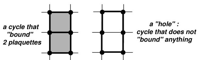
Figure 8: Cycle and hole in FK-configuration.

Equation (6.1) shows that the Euler-Poincaré characteristic of a bond configuration depends only on homotopy equivalence classes of objects and as such, it is an intrinsic property which provides a distinguished signature of its topological features. The fact that it allows to probe the critical behaviour of physical systems makes possible the interpretation of phase transition on purely topological grounds.

This formalism of cell complexes has been shown to be very useful in order to define general duality arguments in several models of statistical mechanics and it is the basis of the algebraic approach of the study of phase transitions [Wa3].

References

- [A] P. S. Alexandroff, Combinatorial Topology, Graylock Press, Rochester, (1956).
- [Ag] M. K. Agoston, Algebraic Topology, Pure and Applied Mathematics, M. Dekker Inc. , New York, (1976).
- [AKPM] C. H. Arns, M. A. Knackstedt, W. V. Pinczewski, and K. Mecke, Phys. Rev. E 63, 31112, (2001).
- [Ba] I. Balberg, Phys. Rev. B 31, 4053, (1985).
- [Bax] R. J. Baxter, J. Phys. C 6, L445, (1973), J. Phys. A 15, 3329, (1982)
- [Be] C. Berge, Graphs and Hypergraphs, North Holland, (1976).
- [FK] C. M. Fortuin and P. W. Kasteleyn, Physica 57, 536, (1972).
- [Gra] S. B. Gray, I.E.E.E. Trans. Comp. 20, 551, (1971).
- [Gri] G. Grimmett, Percolation, Springer, (1999).
- [Ha] H. Hadwiger, Vorlesungen über Inhalt, Oberfläche und Isoperimetrie, Springer, 1957.
- [HK] T. Hofsäss and H. Kleinert, J. Chem. Phys. 86, 3565, (1987).
- [Ho] J. Hoshen, R. Kopelman, Phys. Rev. B 14, 3438 (1976).
- [J] J. P. Jernot and P. Jouannot, in: Mathematical Morphology and Applications to Image Processing. ISMM’94, 35, (1994).
- [K] R. Kotecky and S. Shlosman, Commun. Math. Phys. 83, 493, (1982).
- [KLMR] R. Kotecky, L. Laanait, A. Messager, J. Ruiz, J. Stat. Phys. 58, 199, (1990).
- [LMR] L. Laanait, A. Messager, and J. Ruiz, Commun. Math. Phys. 105, 527, (1986).
- [LMMRS] L. Laanait, S. Miracle-Solé , A. Messager, J. Ruiz, and S. Shlosman, Commun. Math. Phys. 140, 81, (1991).
- [M1] K. R. Mecke, Applications of Minkowski Functionals in Statistical Physics, in Statistical Physics and Spatial Statistics. The Art of Analyzing and Modeling Spatial Structures and Pattern Formation, Lecture Notes in Physics 554, K. R. Mecke and D. Stoyan Eds. Springer (2000).
- [M2] K. R. Mecke, Complete Family of Fractal Dimensions Based on Integral Geometry, submitted to Physica A (2000).
- [MW] K. R. Mecke and H. Wagner, Euler Characteristic and Related Measures for Random Geometric Sets, J. Stat. Phys. 64, 843, (1991).
- [O] B. L. Okun, J. Stat. Phys. 59, 523, (1990).
- [PS] G. E. Pike and C. H. Seager, Phys. Rev. B 10, 1421, (1974).
- [S] L. A. Santalò, Integral Geometry and Geometric Probability, Addison-Wesley, (1976).
- [Sa] S. Fortunato and H. Satz, Polyakov Loop Percolation and Deconfinement in SU(2) Gauge Theory, Phys. Lett. B 475, 311 (2000); S. Fortunato, F. Karsch, P. Petreczky, H. Satz, Effective Z(2) Spin Models of Deconfinement and Percolation in SU(2) Gauge Theory, Phys. Lett. B 502, 321 (2000).
- [Sch] R. Schneider, Convex Bodies: The Brunn-Minkowski Theory, Cambridge University Press, Cambridge (1993).
- [Se] J. Serra, Mathematical Morphology, Academic Press, (1982).
- [SyEs] M. F. Sykes and J. W. Essam, Exact Critical Percolation Probabilities for Site and Bond Problems in Two Dimensions, J. Math. Phys. 5, 1117-1121, (1964).
- [Wa1] H. Wagner, Euler Characteristic for Archimedean Lattices, (2000). (unpublished)
- [Wa2] K. R. Mecke Th. Buchert and H. Wagner, Asrton. Astrophys. 288, 697, (1994).
- [Wa3] K. Drühl and H. Wagner, Ann. Phys. 141, 225 (1982).
- [We] F. J. Wegner, J. Math. Phys. 12, 2259 (1971). (1982).
- [Wo] U. Wolff, Phys. Rev. Lett. 62, 361 (1989).
- [Wu] F. Y. Wu, Rev. Mod. Phys. 54, 235 (1982).