Van Hove Singularity and Superconductivity in Disordered Hubbard Model
Abstract
We apply the Coherent Potential Approximation (CPA) to a simple extended Hubbard model with a nearest and next nearest neighbour hopping for disordered superconductors with –, – and –wave pairing. We show how the Van Hove singularities in the electron density of states enhance the transition temperature for exotic superconductors in a clean and weakly disordered system. The Anderson theorem and pair–breaking effects in presence of Van Hove singularity caused by non–magnetic disorder are also discussed.
pacs:
Pacs. 74.62.Dh, 74.20-zI Introduction
Magnetic and non–magnetic impurities in superconductors always attracted interest and their treatment played the essential role in theories of superconductivity.
Since the Anderson [1] and Abrikosov, Gorkov [2] works the influence of magnetic and non–magnetic disorder on superconductors have been treated in many ways [3, 4, 5, 6, 7, 8, 9]. Their arguments, originally applied to classic BCS superconductors, were reexamined for novel, exotic superconductors [10, 11] with the anisotropic order parameters extended –wave, –wave character [4, 12, 13, 14, 15, 16, 17, 18, 19, 20, 21, 22, 23, 24, 25, 26, 27] and also recently discovered [28, 29, 30, 31] –wave ruthenates [5, 32, 33, 34, 35]
Examining the influence of various kinds of magnetic and non–magnetic disorder caused by structural, substitutional, irradiation defects etc. on properties of conventional and unconventional superconductors has shown that their responses to disorder are quite different. In contrast to conventional materials where only magnetic impurities affect the superconducting properties, for unconventional superconductors the effect of both magnetic and non-magnetic disorder is usually strong [36, 37, 38, 39, 40, 41, 42, 43, 44, 45, 46, 47, 48, 49, 50, 51].
Thus, it is not surprising, that the response to disorder become the fundamental criterion of unconventionality of the physical mechanism leading to superconductivity. Moreover, effects of disorder are of interest because the high temperature superconductors have to be doped (La2-x SrxCuO4 with Strontium , YBa2Cu3O7-x with Oxygen ) to show the optimal critical temperature and doping is always accompanied by disorder.
On the other hand in these quasi two dimensional layered materials the Fermi energy has been found in the vicinity of Van Hove singularities of the electron density of states [52, 53, 54, 55, 56, 57, 58, 59, 60, 61, 62, 63, 64, 65, 66, 67]. This has lead to formulation of Van Hove scenario for high temperature superconductors which says that optimal critical temperature is reached when chemical potential passes through the Van Hove singularity in the density of states [52, 53, 58, 19]. Doping with charge carriers does not only change the density in the system but also smear the density of states eliminating its singularities and, specially for anisotropic superconductors, introduce the electron pair–breaking phenomenon [12, 4, 6, 20].
Thus, one has to investigate the effect of rise and fall of the critical temperature near the Van Hove singularities very carefully, simultaneously, taking into account the effects of disorder. Clearly disorder reduces the critical temperature by elimination of singularities in the density of states and, at the same time, by braking pairs. The present paper is the extension of the previous ones [19, 20, 34] where the electron hopping was introduced only between nearest neighbour lattice sites. Here following Refs. [68, 69] we introduce the hopping to next nearest sites (i.e. the ratio of hopping parameters , for YBaCuO was suggested to be ) and investigate the effect of disorder on superconducting properties.
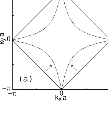
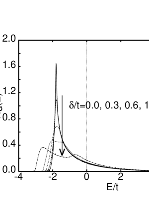
In the normal states the nonzero hopping to the next neighbour sites introduces the distortion of the Fermi surface (Fig. 1a) which results in considerable changes in the electron density of states (Fig 1b). Note, in case the central Van Hove singularity produces the stronger enhancement of the density of states ( for ) than for (Fig. 1b). Moreover, the other Van Hove singularity associated with the bottom edge of the band creates the second peak in the density of states . Thus, depending on the band filling, the additional electron hopping should have the effect on critical temperature , rising it to higher value. On the other hand, the distorted Fermi surface with the stronger dependence on (Fig. 1a) seems to be less stable in the presence disorder as is not a good quantum number in disordered system.
The present paper is organized as follows. In Section II the discussion starts with the extended attractive Hubbard model defined on the square lattice which has the extended – – and – wave order parameter solutions. Than we shortly overview and classify various types of Van Hove singularities in electron density of states of one band model and their influence on the superconducting critical temperature . In Section III we investigate disordered superconducting systems and apply the Coherent Potential Approximation (CPA) for attractive Hubbard model. The Anderson theorem for non-magnetic impurity effect on isotropic –wave solutions and the pair–breaking effect in case of anisotropic pairing is also discussed. Section IV is devoted to the examination of the disorder effect on the superconducting critical temperature . Finally, Section V contains conclusions and remarks.
II The role of Van Hove singularities in the clean system
A Bogoliubov–de Gennes Equation
We start with the single band Hubbard model with an attractive extended interaction which is described by the following Hamiltonian [68, 69, 70]:
| (1) |
In the above is the charge on site labeled , is the chemical potential. Disorder is introduced into the problem by allowing the local site energy to vary randomly from site to site, and are the Fermion creation and annihilation operators for an electron on site with spin , is the amplitude for hopping from site to site (with ) and finally is the attractive interaction () which causes superconductivity and can be either local () or non-local (). Starting from Eq. (1) we apply the Hartree–Fock–Gorkov [71] approximation, which results in the Bogoliubov–de Gennes equation for a singlet (– or – wave) superconductor:
| (2) |
where and are electron and hole wave functions with up anti parallel spins and respectively. The usual singlet one particle Green function, in the Nambu space , at the Matsubara frequency satisfies:
| (3) |
where the pairing potentials will be taken to be non zero only when the sites and coincide (), for on site interaction , or are nearest neighbours, for off diagonal interaction . On the other hand in case of triplet, –wave, paring instead the Eq. 2 we have:
| (4) |
while the analogue of the equation of motion for the Green function in Eq. 3 should be rewritten as:
| (5) |
with the spin dependent 44 Green function. Each of its components is defined as:
| (6) |
The order parameter for triplet paring reads:
| (7) |
We assume that the hopping integrals can take a nonzero values for the nearest and next nearest neighbours. For a clean system can be expressed in -space by Fourier transform: as:
| (8) |
where represents the nearest neighbour site amplitude of electron hopping, while corresponds to next nearest neighbour hopping, denotes the lattice constant, is the chemical potential equal to Fermi energy in zero temperature ( for ). We shall refer to the Greens function matrix as which will be of 22 or 44 size for singlet or triplet solution. The above equations have to be completed by the self-consistency condition for pairing potential:
| (9) |
for singlet pairing case and
| (10) |
for triplet one, where is a positive infinitesimal, is the inverse of temperature and Boltzman constant (in the units we use here ). To simplify matters we have assumed that the Hartree term can be absorbed into the hopping integral and dropped it from Eqs. (2,3) and (4,5). As usual Eqs. (9) and (10) are to be solved together with the corresponding equations for the chemical potential that satisfy the following:
| (11) |
for singles or
| (12) |
for triplets, where is the number of electrons per unit cell.
Here we do not wish to be very specific about the physical nature of the point defects represented by the site energies . We are rather going to provide a reliable analysis of the simplest possible non trivial model. Thus we take them to be independent random variables defined to have values and with equal probability, , on every site [19, 20]. As might be expected we shall be interested in the average of over the above ensemble. To calculate we shall make use of the Coherent Potential Approximation (CPA) which is the best method at hand for the mean field theory of disorder [72].
B Van Hove singularities in clean superconductors
Let’s assume that the sites form a square lattice. Then for clean system ( for all ), in the normal state, where , the spectrum is given by (Eq. 8). It has a saddle point Van Hove singularity at , resulting in the logarithmic divergence of the density of states (Fig. 1b) The density of states for a normal state is defined as:
| (13) |
where is an element of Fermi surface (Fig. 2b) reaches its maximum if Fermi surface satisfy the relation . Finally, density of states can be also expressed by the elliptic function of a first kind [65]:
| (14) |
Van Hove singularities in density of states (Eq. 13,14) correspond to three characteristic flat regions of , where . In Fig. 2a we have plotted band energy (Eq. 8). For cuprates the value of next nearest neighbour hopping term is usually considered as . Here we have chosen (Eq. 8). One can easily determine Van Hove singularities for saddle points: , and these corresponding to band edges: the bottom as well as top one . Three isoenergetic contours ’3’, ’2’, ’1’ have been marked in Fig. 2a for , , . They correspond to Fermi surfaces (Fig. 2b) for three values of band filling , , respectively. Note that for , the Fermi surface has hole like characteristics while for , it corresponds to electron like system. For the Fermi energy passes through the Van Hove saddle point singularity.
For the ’on-site’ attraction (negative ) the linearized gap equation (Eq. 9) at can be written as:
| (15) |
where , and is a critical temperature.
If the interaction is off diagonal then the Fourier transform of leads to following expression:
| (16) |
where
| (17) | |||||
| (18) |
The pairing parameters for corresponding symmetry of solution: extended – – or –wave one have the following form:
| (19) | |||||
| (20) | |||||
| (21) |
and is a Fourier transform of the matrix (Eq. 7). Despite of different types possible solutions described by Eqs. (3,5,20) the linearized gap equation for the critical temperature can be written in a compact form:
| (22) |
depending on the solution symmetry .
The normal density of states and the corresponding projected densities (, and ) used in Eq. (22) can be expressed in terms of Green functions of the normal system as follows:
| (23) | |||||
| (24) | |||||
| (25) | |||||
| (26) |
To calculate the above densities of states we have used the recursion method described in the Appendix A. The appropriate densities of states for the clean system , are plotted in Fig. 3a. Figure 3b shows the –wave projected density in comparison to .
The full line, in Fig. 3a, corresponds to the electron density of states with the spectral dependence of (Eq. 4) and . The position of the central Van Hove singularity (Fig. 2) corresponds to band filling . Apart from that singularity one can see another sharp peak in the lower edge of band and much smoother one in the upper edge. Both of them are singularities of band edges: bottom and top respectively. For the ’on site interaction’ the shape of in Fig. 3a and the gap equation (Eq. 15) indicates that the critical temperature should be enhanced effectively around first two singularities for relatively low electron densities . As a matter of fact such situation can be seen in calculations of (Fig. 4, clean system for curves denoted by ’1’). The critical temperature obtained from the Eqs. (22,24) for various symmetries of the order parameter are depicted in Fig. 4a-c by lines denoted by ’1’ as a function of band filling . Figure 4a corresponds to extended –, – wave cases while Fig. 4b shows to the –wave solution. In this case there exists a maximum in projected density of states close to Van Hove singularities in but it is not so sharp as in or and because of the additional smearing term in the formula for (Eq. 24 ). Nevertheless, this secondary peak also produces the enhancement of critical temperature (Fig. 4b). For comparison, in Fig. 4c we present for an isotropic ’on-site’ – wave solution. Clearly, these calculations support the Van Hove singularity scenario. Note that for relatively low temperature Van Hove singularity is passing at (Figs. 2, 3a). The lack of the particle-hole symmetry results in the shift of maximum value of to higher value of electron densities so in the optimal doping the superconductor is hole superconductor.
Moreover for we observe the degradation of critical temperature . In in this limit of slowly changing density of sates we can apply the result for the constant density of states:
| (27) |
where denotes the bandwidth and is the Heaviside step function.
For small ’on site’ attractive interaction , the critical temperature is given by the analytic formula [68, 70]:
| (28) |
In our case, due to the asymmetry of the electron density of states for the degradation of is faster .
The Van Hove singularities in the spectrum show up also in the projected densities of states , (Fig. 3a). Due to the factors and (Eqs. 18,24) the dependences are severely modified (Fig. 4a, curve ’1’). Moreover, the maximum value of (Fig. 3b) is also close to the Van Hove singularity and it results in the optimum of (Fig. 4b, curve ’1’).
It is worthwhile to notice here that singularities in the band edges are important for an extended –wave case while the saddle point one, located in the middle of the band, for –wave pairing, similarly to an isotropic –wave case.
The positions of the Van Hove singularities result in the strong band filling dependence of (Fig. 2b). Again the pairing dominates in selected regions of . In case of –wave it is the middle region of while for extended –wave pairing it is rather low electron densities region (). The high electron density ( ) is also possible however the is much smaller. Same relation, as in the ’on-site’ pairing case, governs the basic behaviour (Eq. 28). However should be substituted by the corresponding projected density of states . Thus, away the Van Hove singularity, ():
| (29) |
In all cases the Van Hove singularities play the mayor role and could be identified as the source of a critical temperature raise. Its dependence on doping should be described rather by strongly changing function contrasting with the case of a constant density of states (Eq. 14) where is simply .
However it is also worthwhile to note that depending on the paring symmetry different Van Hove singularities can matter and because of non symmetric character of densities of states this effect is approximate. Due to the this asymmetry we observe the additional shift of the optimal doping toward the center of a band. Interestingly, different Van Hove singularities and corresponding shifts depend on solution type and the interaction range. Eventually, an extend ed –wave solution appears to be an electron superconductor while –wave can be identified as hole one.
The formulae for a critical temperature (Eqs. 22) are based on the integral over the appropriate DOS which posses Van Hove singularities. The effect of shift is stronger for smaller where hyperbolic tangent is smearing the function under integrals. It is also worth to note that Van Hove scenario is working better for superconductors with relatively small transition temperature (which corresponds to a small interaction parameter ). This can easily be seen from the following function:
| (30) |
present in the gap equations (9,12). It can be interpreted as leading to a natural cut-off around the chemical potential . Note that if the temperature is small then the function is non zero in the narrow range of energies around only. In fact in the limit it tends to the Dirac delta function () and the cut-off is limited to the neighbourhood of the point. Note, that for finite , . Consequently, for the logarithmic Van Hove singularity in the density of states near has the form:
| (31) |
and we get the Labbe–Bok formula for [55, 58, 56]:
| (32) |
III CPA for disordered Hubbard Model
As mentioned above, the technical question we shall answer in this paper is what happens to above behaviour when the site energies are not the same on all sites but are randomly distributed. For example in a binary alloy, , we have random distribution of site energies: depending on occupation at the site by atom or with probabilities and respectively. Such problem have been dealt with within the Coherent Potential Approximation (CPA) on a number of occasions in the past [73, 74, 75, 76, 77, 78, 18, 19, 20, 34]. Here we shall follow the usual arguments generalized as appropriate. In short, we shall take the CPA to mean that the coherent potential [72], in a site approximation, is defined by the zero value of an averaged t-matrix . Namely
| (33) | |||||
| (34) |
where specifies the occupation of the site and hence the disordered potential .
In case of ’on site attraction’ (Eq. 1 with ). In the limit of small fluctuations in the paring potential (), a constant averaged value
| (35) |
can be applied.
Using now CPA equations equations (Eqs. 33 and Appendix B) it can be readily shown that due to the disorder and in the clean limit is renormalized to and in the same way
| (36) | |||||
| (37) |
On account of the general symmetry between the the averaged Green function elements and that of the coherent potential , for complex energies, it follows that
| (38) |
| (39) |
Note that one can write Eq. (36) in terms of Matsubara frequencies ():
| (40) |
where
| (41) |
Eventually Eq. (39) leads to the linearized gap equation (Appendix B):
| (42) |
This equation relates directly to the similar one of the clean case (Eq. 15) with the difference due to the substitution of the density of states for the pure system by the averaged one of the doped material . Evidently, assuming small fluctuations in the the pairing potential (Eq. 35) one gets a critical temperature weakly depending on disorder. This is the content of the Anderson theorem [3, 79] which rests on the assumption that pairing potential does not fluctuate in space for all . However, it should be noted that in short coherence length limit the situation can be opposite. In that case allowing the spatial fluctuations of the pairing amplitude induced by the site energy disorder or introduced by the randomly distributed attractive centers ( for some lattice sites ) the Anderson theorem breaks down even for conventional, on site, –wave superconductors [78, 77].
For a constant pairing parameter as in Eq. (35) the generic consequence of disorder in the system with on site attraction is the smearing of the structure in the averaged density of states (Eq. 42). To illustrate the consequences of it in our model we have calculated using the standard CPA procedure [76, 19, 20] for , , .
The results for various values of the scattering strength leading to the smearing of the Van Hove singularities in the averaged density of states , are shown in Fig. 5a. Van Hove singularities are still present here for a relatively weak disorder strength while for stronger one one can notice additional splitting of singularities caused by the model of disorder. This is the so called the split band regime [72, 78]. Namely the two peaks are the remnant of the Van Hove singularities of the two, A and B, pure metals.
Let us now examine a disordered system with the inter-site attraction . Here we assume that inter-site pairing parameter can be substituted by its average [18, 19, 20]. Thus, in the case of a singlet paring (extended – or – wave), the on site impurity potential can be expressed as
| (43) |
while the coherent potential matrix has the form:
| (44) |
Naturally, the averaged Green function, can be expressed as follows:
| (45) |
In case of triplet pairing (–wave) instead Eqs. (43-45) the following notation should be introduced [34, 35]
| (46) |
for the impurity potential and the coherent potential
| (47) |
respectively. Again the averaged Green function is given by
| (48) |
while the conditionally averaged Green function at the impurity site ( or ) has the following form:
| (49) |
The averaged paring parameters can be written as in (Eqs. 20):
| (50) | |||||
| (51) | |||||
| (52) |
| (53) |
for singlets (extended – and – wave) and
| (54) |
for triplets (–wave) cases.
From Eqs. (45) and (48) it follows that off diagonal elements of the Green function are
| (55) |
for singlets and
| (56) |
for triplets, where or .
Interestingly, the linearized gap equation can be written as in a way similar to that for the clean system (Eq. 22):
| (57) |
where the imaginary parts of define the projected densities of states for a disordered system , and discussed in Appendix A. Moreover, as in case of clean system (Eqs. 24):
| (58) |
where or depending on the symmetry of solution: extended –, – and –wave. Figures 5b–d show the corresponding projected densities of states of a disordered system (Eq. 58): , and . Like for (Fig. 5a) for weak disorder, Van Hove singularities survive. Thus, it is clear that the smearing of the Van Hove singularity in Figs. 6a-d implies a weakening of the Van Hove enhancement of the critical temperature .
For our simple model of disorder of binary alloy AcB1-c with c=0.5 the coherent potential , satisfies the following CPA equation [72]:
| (59) |
In Fig. 6a,b we also show the corresponding self energy which in one site CPA depends only on energy but not on the wave vector . One can see that for a relatively weak disorder strength the maximum of is exactly at Van Hove singularity as in the Born approximation [12, 19, 20]:
| (60) |
The above result is valid also below the critical temperature because for off diagonal pairing [19, 20] and (Eq. 59) is still valid.
In case with a larger disorder strength the maximum of is located in some other energy according to the model of disorder we use (Eqs. 1, 43-49). Simultaneously the real part of self energy is changing with energy renormalizing the chemical potential (Eq. 58).
Let us investigate the additional effect of disorder visible in Eq. (57). Comparing this equation with the clean system one (Eq. 22) one can notice the difference in the denominator, where in case of disordered system there is an additional strong scattering term .
To examine it further let us rewrite the gap equation in terms of Matsubara frequencies :
| (61) |
for – – and –wave symmetry.
Now, let us approximate the normal state self energy and projected density of states by:
| (62) | |||||
| (63) | |||||
| (64) |
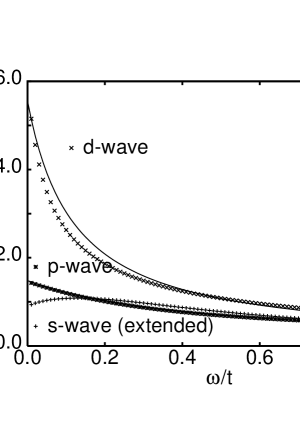
In Fig. 7a we have plotted the densities versus imaginary part of energy for Fermi energy chosen at Van Hove singularity ().
Note that in that region we can roughly approximate the corresponding projected densities by a simple formula
| (65) |
where and are constants depending on the pairing symmetry . Introducing Eq. (65) and Eqs. (62,63) into Eq. (61) we get:
| (66) |
Now we have to perform the summation over for clean and disordered cases . After some algebra (Appendix C) we get the approximate pair–breaking formula:
| (67) |
Note that in the limit the constant density of states const. (Eq. 65), , we get automatically the the standard Abrikosov–Gorkov formula [3] with a characteristic pair–breaking parameter :
| (68) |
In Eqs. (67 and 68) denotes the critical temperature in a clean system, while is the critical temperature in dirty one.
In Fig. 7b we plot versus for few values of . Here the chemical potential was fixed at the saddle point Van Hove singularity . Interestingly, the slop of the curve (Fig. 7b) is increasing with decreasing indicating that in presence of Van Hove singularities for a disordered system we get weaker decreasing of than for a flat density of states. Thus, for -wave pairing and for –wave superconducting phase is more stable than in case of extended –wave pairing, where (Fig. 7a). This is the main result obtained in this section. In spite of very rough approximation used here the results show that the Van Hove singularity influences the pair–breaking effect. Namely it makes superconductivity more robust increasing the critical strength of disorder needed to break the Cooper pairs.
IV Critical Temperature for Disordered superconductors
Let us now turn to the case where both superconductivity and disorder are present[73, 74, 75, 76] and calculate the critical temperature self-consistently. Although the full CPA program can be implemented for the problem defined by Eqs. (9-10 and B.1-B.4) [76, 78] and the specification of the site energy ensemble, it is convenient to make the approximation, valid when the coherence length is much larger then the lattice spacing, that the pairing potential does not fluctuate very much and replace it in equations (3 and 5) by its average value [79]. For conventional isotopic –wave pairing the gap equation at takes the simple form (Eq. 42). Thus, the critical temperature at the optimal doping should be only slightly reduced by disorder due to smearing of the density of states . The results of numerical calculations for four different values of a disorder strength in case of the ’on site’ attraction is presented in Fig. 4c. Clearly, in this case the critical temperature is sightly reduced by the effect of the density of states.
On the other hand for the ’off diagonal’ attraction case the linearized gap equation, in presence of disorder, is given by the formula (Eq. 57). Solving it for extended – – and – wave pairing symmetries we get the critical temperature versus band filling. The results for various are presented in Fig. 4a (extended – and –wave) and 4b (–wave). Here, we observe significant degradation of in all three anisotropic pairing cases. Moreover, in some regions of electron concentration, disappearing of a supercondacting phase can be noticed for relatively weak disorder (). Especially this happens to the –wave case with high electron concentration and as well as the –wave case for (Fig. 4a). The dramatic degradation of extended –wave superconductivity for can be also seen for stronger disorder (). In that region of electron concentration , due to the binary alloy model of disorder AcB1-c and , the position of energy for the maximum of a pair–breaking term (Fig. 6) coincides with the chemical potential making the pair–breaking mechanism very efficient. Similar behaviour can be seen for –wave superconductor (Fig. 4b). Clearly, for large enough (Fig. 4a–b) the superconductivity is destroyed by the pair-breaking effect shrinking the region of for . In the same time the corresponding projected densities are not strongly effected (Fig. 5). The results for anisotropic paring in Figs. 4a–b are contrasting with Fig. 4c where we plotted the results for the on site solution with . Here, (Fig. 4c) the region of band filling , where a superconducting solution exists, does not change with disorder at all.
V Conclusions and Remarks
We have analyzed the effect of disorder on disordered Hubbard model with local and non-local, nearest neighbour, interactions as well as nearest and next neighbour electron hopping terms. We have got numerical and analytical results confirming previous works on the similar model with a simple band energy [19, 20] . Such dispersion relation, introduces the electron-hole symmetry for half filled band and locates the saddle point Van Hove singularity exactly in the center of the band (Figs. 1a,b). Including the additional hopping , we break the electron hole symmetry in the densities of states, resulting in shifting the central Van Hove saddle point singularity to the bottom of the band. In the same time another Van Hove singularity, located at the bottom band edge, appears to be important. Thus the effect of Fermi surface distortion make place both of singularities very close to each other For some of band filling values both of singularities play important roles. It is clear after analyzing the appropriate projected densities of states . Moreover various pairing symmetries choose different Van Hove singularities. -wave symmetry is favored in case of the regions of band fillings with chemical potential near the saddle point singularity while extended – wave pairing symmetry is more likely as far as the bottom edge singularity is concerned. Interestingly, on account of the non-symmetricity of electron density of states the Van Hove scenario is fulfilled only approximately. Here we observe a small interaction dependent, shift of the optimal doping electron concentration towards the center of the band. As a result of the above we conclude that Van Hove singularity is important for all discussed symmetries of order parameter. Interestingly, in presence of an additional electron hopping to the next nieghbour lattice site , the shift of the saddle point Van Hove singularity in the density of states explains that the superconductor with an extended –wave symmetry is rather of electron type while with –wave symmetry case is of hole nature. Note also that, the positions of the maximum value of , , (Fig. 5) are not affected by small disorder. In spite of small density of states effects leading to smearing peaks in corresponding densities: , and (Eq. 58, Fig. 5), the critical temperature , plotted in Figs. 4a–b, is degradated strongly with disorder. This is due to the pair–breaking term (Eq. 61). In the negative , ’on-site’, interaction there is a quite different situation. Here disorder causes only small decrease of (Fig. 4c) via a density of states effect (Fig. 5a). So, the most interesting effect arises from Eqs. (61,66), where acts as a pair breaker.
Concluding our results we would like to stress that the Van Hove singularity does not make the decrease in more pronounced as one can expect (because of singularities are present in the self energy , Fig. 6). In fact singularities make it weaker. We have analyzed this effect very carefully in Sec. III finding an approximate pair–breaking formula (Eq. 67). Here, the Van Hove singularity influenced the pair–breaking Abrikosov–Gorkov curve, changing its slope of the versus . Similar effect has been observed in the experimental results for Zn–doped LSCO [49]. Alternatively, this effect can be also explained assuming anisotropic scattering potentials [6, 7].
Finally, we observed the dependence of on band filling . Our results for –wave superconductor show that the Van Hove scenario is valid even in presence of weak disorder (Figs. 4). Similar experimental results were obtained by measuring , in various cuprate compounds, as a function of hole concentration where Cu were substituted by Zn [41, 42]. The concentration of Zn was there the measure of disorder.
It should be however noted that high cuprates are strongly correlated electron systems and the mean field approach basing on the effective intersite attraction , presented here has a limited applicability [69]. Strictly speaking a more realistic model should posses, beside an intersite attraction, a strong Coulomb repulsion term. Although the approximations we used in the present paper aimed to explain the effect of the Van Hove singularity in a presence of disorder in a weak coupling regime, the preliminary calculations using simultaneously slave boson technique and CPA [81] seams to support the general arguments of the Van Hove singularities significance for superconducting cuprates conjectured here.
A Appendix
In this Appendix we apply the recursion method to calculate appropriate densities of states. Let us investigate the projected densities if states , , and the corresponding Green functions: , and :
| (A.1) | |||||
| (A.2) | |||||
| (A.3) |
where and were defined in Eq. 11.
Noting trigonometric identities:
| (A.4) | |||||
| (A.5) | |||||
| (A.6) |
the Green functions , and can be easily found as a combination of diagonal and off diagonal Green functions , see the notation in the schematic picture (Fig. 8):
| (A.7) | |||||
| (A.8) | |||||
| (A.9) |
Function , and have been calculated using the recursion method [80, 19, 20].
B Appendix
In this Appendix we apply CPA equations (Eqs. 20-27) to the disordered Hubbard model with the ’on site attraction’ Eq. 1 () and discuss the Anderson theorem [1, 79]. The averaged Green function, can be expressed as follows:
| (B.1) |
while conditionally averaged Green function has the form
| (B.2) |
The disordered potential in Eq. 20 has the following form [76, 77, 78]:
| (B.3) |
where or corresponds to different site energies of the lattice site while or relates to the different paring potential in an alloy .
Clearly, the coherent potential can be written as
| (B.4) |
Function can be obtained from Eq. B.1
| (B.5) |
substitution of Eq. B.6 and B.7 into the right and left hand sides of Eq. B.5 respectively an equation on and :
| (B.8) |
Using B.6 and factorizing of above we get:
| (B.9) |
In the limit of small paring potential fluctuations it can be used as a constant to satisfy the Anderson theorem. Then
| (B.10) |
and renormalized quantities of and reads as:
| (B.11) | |||||
| (B.12) |
This lead to the same renormalization in the pair potential and energy :
| (B.13) |
| (B.14) | |||||
| (B.15) |
and the linearized gap equation
| (B.16) |
where denotes normal state DOS:
| (B.17) |
C Appendix
In this Appendix we apply CPA to anisotropic superconductor and evaluate the approximate formula of the pair–breaking effect. Starting from the clean system we assume that the linearized gap equation can be written (Eqs. 63-68) by:
| (C.1) | |||||
| (C.2) |
where is a cut-off in the summation (C.1) As is very large, it yields
| (C.3) |
On the other hand for disordered system we have:
| (C.4) | |||||
| (C.5) |
Similarly (to Eqs. C.1,C.3) it leads to
| (C.6) |
and finally comparing Eqs. (C.3 and C.6) we get
| (C.7) |
where is a pair–breaking parameter
| (C.8) |
and is the critical temperature for a clean superconductor.
ACKNOWLEDGMENTS
This work has been partially supported by KBN grant No. 2P03B09018. A part of this work has been done during the stay in the Abdus Salam International Centre for Theoretical Physics in Trieste. The author would like to thank Prof. K.I. Wysokinski, Prof. B. L. Györffy and Dr. J.F. Annett for helpful discussions.
REFERENCES
- [1] P.W. Anderson, J. Phys. Chem. Solids 11, 26 (1959).
- [2] A.A. Abrikosov and L.P. Gorkov, Sov. Phys. JETP 8, 1090 (1959).
- [3] K. Maki in Superconductivity, edited by R.D. Parks (Marcel Dekker, New York 1969) Vol. 2, Chapter 8.
- [4] Y. Sun and K. Maki, Phys. Rev. B 51, 6059 (1995).
- [5] K. Maki, S. Haas, Phys. Rev. B 62 R11962 (2000).
- [6] G. Harań and A.D. Nagi, Phys. Rev. B58, 12 441 (1998).
- [7] G. Harań and A.D.S. Nagi, Phys. Rev. B 6301, 2503 (2001).
- [8] D. Belitz and T.R. Kirkpatrick, Rev. Mod. Phys. 66, 261 (1994).
- [9] A. Ghosal, M. Randeria, and N. Trivedi, Phys. Rev. B 6303 7301 (2001).
- [10] J.F. Annett, N. Goldenfeld and A.J. Leggett in Physical Properties of High Temperature Superconductors, edited by D.M. Ginsberg (World Scientific, Singapore, 1996) Vol. 5.
- [11] J.F. Annett Physica C 323, 146 (1999).
- [12] L.P. Gorkov and P.A. Kalugin, JETP Lett. 41, 253 (1983).
- [13] S.V. Pokrovsky and V.L. Pokrovsky, Phys. Rev. B 54, 13275 (1996).
- [14] A.A. Neresysyan, A.M. Tsvelik, and F. Wenger Phys. Rev. Lett. 72, 2628 (1994).
- [15] A.A. Nersesyan, A.M. Tsvelik, and F. Wenger, Nuc. Phys. B 438, 561 (1995).
- [16] A.A. Nersesyan and A.M. Tsvelik, Phys. Rev. Lett. 78, 3981 (1997).
- [17] R. Fehrenbacher, Phys. Rev. Lett. 77, 1849 (1996).
- [18] F. Wenger, Z. Phys. B 98, 171 (1995).
- [19] G. Litak, A.M. Martin, B.L. Györffy, J.F. Annett, and K.I. Wysokiński, Physica C 309 257 (1998).
- [20] A.M. Martin, G. Litak, B.L. Györffy, J.F. Annett, and K.I. Wysokiński, Phys. Rev. B 60 7523 (1999).
- [21] R.J. Radtke, K. Levin, H-B. Schuttler, M.R. Norman, Phys. Rev. B 48, 15957 (1993).
- [22] B.C. Den Hertog and M.P. Das, Phys. Rev. B58, 2838 (1998).
- [23] L.A. Openov, Pis’ma Zh. Eksp. Teor. Fiz. 66, 627 (1997).
- [24] L.S. Borkowski and P.J. Hirschfeld, Phys. Rev. B 49, 15404.
- [25] L.A. Openov, Phys. Rev. B 58, 9468 (1998).
- [26] C. Buhler, S. Yunoki, A. Moreo, Phys. Rev. B 62 R3620 (2000)
- [27] V.M. Loktev, Yu. G. Pogorelov, preprint cond-mat/0104581.
- [28] Y. Maeno, H. Hashimoto, K. Yoshida, S. Nishizaki, T. Fujita, J.G. Bednorz and F. Lichtenberg, Nature 372, 532 (1994).
- [29] G. Baskaran , Physica B 224, 490 (1996).
- [30] D.F. Agterberg, T.M. Rice and M. Sigrist, Phys. Rev. Lett. 78 3374 (1997).
- [31] Y. Maeno, T.M. Rice, and M. Sigrist, Physics Today 54 (2001) 42.
- [32] K. Myake and O. Narikiyo, Phys. Rev. Lett. 83, 1423 (1999).
- [33] E. Puchkaryov, K. Maki, Physica C 341 727 (2000).
- [34] G. Litak, J.F. Annett, B.L. Györffy, Acta Phys. Pol. A 97 (2000) 249.
- [35] G. Litak, J.F. Annett, B.L. Györffy in Open Problems in Strongly Correlated Electron Systems edited by J. Bonca et al. (Kluver, Dordrecht 2001) p. 425.
- [36] K. Westerholt and B. Von Hedt, J. Low. Temp. Phys. 95 123 (1994).
- [37] N. Peng and W.Y. Liang. Physica C 233, 61 (1994).
- [38] K. Uchinokura, T. Ino, I. Teresaki, and Tsakuda, Phyica B 205, 234 (1995).
- [39] E.R. Ulm, J.T. Kim, T.R. Lemberger, S.R. Foltyn and X.D. Wu, Phys. Rev. B 51, 9193 (1995).
- [40] G. Xiao, M.Z. Cieplak, J.Q. Xiao and C. L. Chien, Phys. Rev. B 43, 1245 (1990).
- [41] C. Bernhard, J.L. Tallon, C. Bucci, R. De Renzi, G. Guidi, G.V.M. Williams, and Ch. Niedermayer, Phys. Rev. Lett. 77, 2304 (1996).
- [42] J.L. Tallon, C. Bernhard, G.V.M. Williams, and J.W. Loram, Phys. Rev. Lett. 79 5294.
- [43] Y.K. Kuo, C.W. Schneider, M.J. Skove, M.V. Nevit, G.X. Tessema, and J.J. McGee, Phys. Rev. B 56, 6201 (1997).
- [44] G.V.M. Williams, and J.T. Tallon, Phys. Rev. B 57, 10 984 (1998).
- [45] J. Giapintzakis, D.M. Ginsberg, M.A. Kirk, and S. Ockers, Phys. Rev. B 50, 15967 (1994).
- [46] V.F. Elesin, K.E. Kon’kov, A.V. Krasheninnikov, and L.A. Openov, Sov. Phys. JETP 83, 395 (1996) [Zh. Eksp. Teor. Fiz. 110, 731 (1996)].
- [47] M.Z. Cieplak, K. Karpińska, J. Domagała, E. Dynowska, M. Berkowski, A. Malinowski, S. Guha, M. Croft, and P. Lindenfeld, App. Phys. Lett. 73 2823 (1998).
- [48] K. Karpińska, P-A Vieillefond, M.Z. Cieplak, F. Rullier–Albenque A. Malinowski, and M. Berkowski, Mol. Phys. Reports 20, 91 (1997).
- [49] K. Karpińska, M.Z. Cieplak, S. Guha, A. Malinowski, T. Skośkiewicz, W. Plesiewicz, M. Berkowski, B. Boyce, T.R. Lemberger, and P. Lidenfeld, Phys. Rev. Lett. 84, 155 (2000).
- [50] Z.Q. Mao, Y. Mori, Y. Maeno, Phys. Rev. B 60 610 (1999).
- [51] R.P. Macenzie, R.K.W. Haselwimmer, A.W. Tyler, G.G. Lonzarich, Y. Mori, S. Nishizaki and Y. Maeno, Phys. Rev. Lett. 80, 161 (1998).
- [52] R.S. Markiewicz, J. Phys. Chem. Solids 58, 1173 (1997).
- [53] J. Friedel, J. Phys. Conden. Matter 1, 7757 (1989).
- [54] I.E. Dzialoshinskii, Zh. Eksp. Teor. Fiz. 93 1487 (1987) [Sov. Phys. JETP 66 848 (1987)].
- [55] J. Labbé, J. Bok, Europhys. Lett. 3, 1225 (1987).
- [56] C.C. Tsuei, D.M. Newns, C.C. Chi, and P.C. Pattnaik Phys. Rev. Lett. 65 2724 (1990).
- [57] J. Bok, J. Bouvier, Physica C 282–287, 294 (1997)
- [58] J. Bouvier, J. Bok, in The Gap Symmetry and Fluctuations in High Temperature Superconductors, edited by J. Bok et al., (Plenum, New York 1998).
- [59] J. Bok, J. Bouver, J. Supercond. 13 781 (2000).
- [60] Z. Szotek, B.L. Györffy, W.M. Temmerman, O.K. Andersen, Phys. Rev. B 58 522 (1998).
- [61] O.K. Andersen, O. Jepsen, A.I. Liechtenstein, Phys. Rev B 49, 4145 (1994).
- [62] D.L. Novikov and A.J. Freeman, in Recent Developments in High Temperature Superconductivity, edited by J. Klamut, B.W. Veal, B.M. Dabrowski, P.W. Klamut, M. Kazimierski (Springer, Berlin 1996).
- [63] W.E. Pickett, Physica C 289, 51 (1997).
- [64] D.M. Newns, C.C. Tsuei and P.C. Pattnaik, Phys. Rev. B 52, 13611 (1995).
- [65] D. Quesada, A. Rubio–Ponce, R. Baquero, R. Pena, and C. Trallero–Giner, preprint cond-mat/9905081.
- [66] D. Quesada, R. Peña, C. Trallero–Giner, Physica C 322 169 (1999).
- [67] D.H. Lu, M. Schmidt, T.R. Cummins, S. Schuppler, F. Lichtenberg, and J.G. Bednorz, J. Low Temp. Phys. 105 1587 (1996).
- [68] R. Micnas, J. Ranninger, S. Robaszkiewicz, Rev. Mod. Phys. 62, 1 (1990)
- [69] R. Micnas, S. Robaszkiewicz, in High- Superconductivity 1996: Ten Years after the Discovery, edited by E. Kaldis, E. Liarokapis, K.A. Müller (Kluver, Dordrecht 1997) p. 31.
- [70] R. Micnas, J. Ranninger, S. Robaszkiewicz, S. Tabor, Phys. Rev. B 37, 9410 (1988).
- [71] M. Tinkham, Introduction to Superconductivity (McGraw-Hill New York, 1975).
- [72] R.J. Elliot, J.A. Krumhansl, and P.L. Leath, Rev. Mod. Phys. 46, 465 (1974).
- [73] H. Lustfeld, J. Low. Temp. Phys. 12, 595 (1973).
- [74] G. Kerker and K.H. Bennemann, Solid State Commun. 14, 365 (1974).
- [75] K.I. Wysokiński, and A.L. Kuzemsky, J. Low Temp. Phys. 52, 81 (1983).
- [76] G. Litak, K.I. Wysokiński, R. Micnas, S. Robaszkiewicz, Physica C 199, 191 (1992).
- [77] G. Litak, B.L. Györffy, Phys. Rev. B 62, 6629 (2000).
- [78] R. Moradian, J.F. Annett, B.L. Györffy, and G. Litak, Phys. Rev. B 6302 4502 (2001).
- [79] B.L. Györffy, G. Litak and K.I. Wysokiński, in Fluctuation Phenomena in High Temperature Superconductors, edited by M. Ausloos and A.A. Varlamov (Kluver, Dordrecht 1997) p. 385.
- [80] G. Litak, P. Miller, B.L. Györffy, Physica C 251, 263 (1995).
- [81] M. Krawiec, T. Domański, G. Litak and K.I. Wysokiński, Mol. Phys. Reports 34 22 (2001).