Theory of the Quantum Paraelectric – Ferroelectric Transition

Abstract

A realistic theory of the quantum paraelectric – ferroelectric transition is presented, involving parameters determined from band calculations and a renormalization group treatment of critical fluctuations. The effects of reduced dimensionality and deviations from cubic symmetry are determined. Expressions for the pressure dependence of $T_{c}$ as well as $p$ and $T$ dependence of the specific heat are derived, and evaluated for realistic materials parameters for the systems BaTiO₃ and PbTiO₃. In these materials the ferroelectric soft mode dispersion apparently exhibits a very strong cubic anisotropy, which affects results in an important, albeit quantitative, manner. A change in order parameter orientation from (100) to (111) is predicted as quantum criticality is approached.

I Introduction

Ferroelectrics and the closely related high dielectric constant materials are important in many areas of modern technology including memory, sensor and electronic applications, and are of fundamental scientific interest Lines77 . The ferroelectric phase change belongs to a class of structural transitions, generally termed ferrodistortive, triggered by zone-center soft modes of lattice motion. Characteristically the ferroelectric transition involves the condensation of an optically active lattice mode which causes the appearance of long-range polar order and the breaking of the inversion symmetry of the ‘high-temperature’ prototype lattice. One important issue is the ferroelectric quantum critical point, i.e. the physics occurring when, by varying a control parameter $r$ (applied pressure or change of chemical composition), the transition temperature of a ferroelectric is driven to zero. Although a quantum critical point occurs at $T=0$, the fluctuations associated with the critical point may control behavior over a range of temperature and pressure. For example K. A. Müller Mueller79 coined the term “quantum paraelectric” to describe materials in which ferroelectric ordering is prevented by quantal fluctuations. A material just on the disordered side of the $T=0$ ferro-paraelectric transition is therefore an example of a “quantum paraelectric”. The important feature of quantal ($T=0$) phase transitions is that temporal fluctuations must be treated on the same footing as thermal ones Hertz73 ; Sachdev99 . This raises the effective dimensionality and makes the critical behavior more mean-field-like but with temperature dependence controlled by ‘dangerous irrelevant operators’ Millis93 .

Ferroelectric transitions may be described by bosonic field theories with undamped dynamics (if the effect of free carriers may be neglected) and complicated dispersions arising from the long range of the dipolar interaction. Quantum critical phenomena associated with undamped bosonic field theories with short ranged interactions have been extensively studied Sachdev99 . The effect of long range (dipole) forces was studied by Rechester Rechester71 and by Khmel’nitskii and Shneerson Khmelnitskii71 within an approximation equivalent to the self-consistent one loop approximation of Moriya Moriya85 . Aharony and Fisher Fisher73 studied the classical ferroelectric transition and found that anisotropies associated with the dipolar interaction led to a new universality class. In this paper we reexamine the issue in light of recent developments in the theory of quantum critical phenomena. We formulate a realistic action for the ferroelectric soft modes, show how estimates of the parameters may be obtained from ab initio calculations and study quantitatively the consequences of the dipolar-induced anisotropies. Our results agree in essentials with those of Rechester and Khmel’nitskii and Shneerson, but we obtain a more detailed and quantitative picture of the phase boundary, of the effect of anisotropy, and of the logarithmic corrections arising at the marginal dimensionality, which lead to an evolution of the anisotropy as the ordered phase is approached.

II Order parameter and action

The order parameter of our theory is the local polarization ${\bm{\phi}}$. Taking into account the effective dipole charges $e_{i}^{*}$ of the soft modes, ${\bm{\phi}}$ can be formally written

$${\bm{\phi}}(x,t)=\sum_{i=1}^{5}e_{i}^{*}{\bf r}_{i}(x,t).$$ (1)

Here the index $i$ runs through the atoms of the unit cell of the prototype perovskite lattice with stoichiometry ABO₃; ${\bf r}_{i}$ are the vector displacements of each atom.

We now write a Ginsburg – Landau action describing quantal and thermal fluctuations of ${\bm{\phi}}(x,t)$. The crucial point is that because ${\bm{\phi}}$ corresponds to a dipole fluctuation it generates electric fields which lead to a long-range interaction. We have (in space and imaginary time)

$$S[\phi_{\alpha}(x,\tau)] = \int{d^{d}x\over a^{d}}\int_{0}^{\hbar/T}d\tau E_{0}\Big{[}{a^{2}\over c^{2}}\left(\partial_{\tau}\phi_{\alpha}(x,\tau)\right)^{2}$$

$$+ a^{2}\left(\nabla\phi_{\alpha}(x,\tau)\right)^{2}+\phi_{\alpha}(x,\tau)r_{\alpha\beta}\phi_{\beta}(x,\tau)$$

$$+ \int{d^{d}x^{\prime}\over a^{d}}\phi_{\alpha}(x,\tau)F_{\alpha\beta}(x-x^{\prime})\phi_{\beta}(x^{\prime},\tau)$$

$$+ \sum_{\alpha\beta}\left(u+v_{\alpha}\delta_{\alpha\beta}\right)\phi_{\alpha}^{2}(x,\tau)\phi_{\beta}^{2}(x,\tau)\Big{]}+...$$

Here $a$ is the lattice constant, $c$ is the speed of the phonons in the softest direction, and $E_{0}=\hbar c(\pi/a)$ is the typical energy scale of ferroelectric fluctuations in the (100) direction; our choice of units is such that the field, mass and coupling constants are dimensionless. The term proportional to $F_{\alpha\beta}(x)=(d-2)(x^{2}\delta_{\alpha\beta}-dx_{\alpha}x_{\beta})/x^{d+2}$ represents the dipole interaction. In momentum space Fisher73

$$F_{\alpha\beta}(q) = \int d^{d}xF_{\alpha\beta}(x)e^{i{q\over a}\cdot x}=\left(r_{0\alpha}+f_{\alpha}q_{\alpha}^{2}\right)\delta_{\alpha\beta}$$

$$+\left(g_{\alpha\beta}-q^{2}h_{\alpha\beta}\right){q_{\alpha}q_{\beta}\over q^{2}}+{\mathcal{O}}(q^{4}),$$

where $r_{0\alpha}$, $f_{\alpha}$, $g_{\alpha\beta}$, and $h_{\alpha\beta}$ depend on details of the underlying lattice. We assume that the non-local quadratic terms represented by $g_{\alpha\beta}$ and $h_{\alpha\beta}$ obey the same symmetry as the local quartic interaction terms $u+v_{\alpha}\delta_{\alpha\beta}$. Thus, in general, we will have $g_{\alpha\beta}=g+g_{I}\delta_{\alpha\beta}$; $g_{I}>0$ lowers the symmetry to Ising. The term $r_{0\alpha}$ combined with local bare mass terms makes up $r_{\alpha\beta}$ in Eq. (II). We shall consider cubic and tetragonal symmetry, so $r_{\alpha\beta}=r_{\alpha}\delta_{\alpha\beta}$. In Eq. (II) and in all of the following we use dimensionless momenta $q_{\alpha}\in[-\pi,\pi]$.

Diagonalization of the quadratic part of the action yields the phonon modes, and the paraelectric – ferroelectric transition occurs when the lowest zone center mode frequency vanishes. The gradient term in Eq. (II), along with $f_{\alpha}$ and $h$, controls the dispersion of modes. Note that $f_{\alpha}\neq 0$ implies an anisotropic derivative $\sum_{\alpha}(\nabla_{\alpha}{\bm{\phi}}_{\alpha})^{2}$; in a spherically symmetric system $f_{\alpha}=0$. For simplicity we refer to the case $g_{I}=0$, $f_{\alpha}>0$ as Heisenberg also, because the order parameter exhibits a continuous rotational symmetry. Previous renormalization group studies of the classical paraelectric – ferroelectric transition have treated the $f_{\alpha}$-terms as a small perturbation Fisher73 ; Khmelnitskii71 . Khmel’nitskii and Shneerson Khmelnitskii71 argue that although $f_{\alpha}$ in typical materials (e.g. BaTiO₃) is of the same order of magnitude as $g_{\alpha\beta}$ and $h_{\alpha\beta}$, the anisotropy of observable quantities is usually weak. Because band theory calculations indicate that in many ferroelectric systems $f_{\alpha}>1$ are quite large we present here a treatment valid for any $f$.

The $u$ and $v_{\alpha}$ terms represent local anharmonic interactions. The materials of main interest here have cubic symmetry in which case $v_{\alpha}=v$. The quartic interaction in Eq. (II) (dropping momentum and energy integrals for simplicity) becomes

$$S^{(4)}[{\bm{\phi}}]=u\left(\sum_{\alpha}\phi_{\alpha}^{2}\right)^{2}+v\sum_{\alpha}\phi_{\alpha}^{4}$$ (4)

The term proportional to $u$ is rotationally invariant and insensitive to the polarization orientation, and the sign of the second term determines the polarization orientation in the ordered phase. At the mean field level the action Eq. (II) is minimized by polarization of magnitude

$$P^{2}=\sum_{\beta}\phi_{\beta}^{2}=-{dr\over 2(du+v)}$$ (5)

When $v<0$ Eq. (II) is minimized by a polarization along (111) with $\phi_{x}=\phi_{y}=\phi_{z}=P/d$ whereas for $v>0$ the polarization is along (100) with $\phi_{x}=\phi_{y}=0$, $\phi_{z}=P$. The values of the quartic interaction are in each case

$$S^{(4)}[{\bm{\phi}}]={(dr)^{2}\over 4(du+v)}\times\begin{cases}\left(u+v/27\right),&v<0\\ \left(u+v\right),&v>0\end{cases}$$ (6)

The condensation energy is of order $r^{2}/u$ and as $v\to 0$ the energy barrier separating different symmetry-allowed polarization directions is a factor of order $v/u$ smaller than the condensation energy. The condition for the stability of a quartic interaction is the positive definiteness of Eq. (4) which (in cubic symmetry, dimensionality $d$ and at the mean field level) translates into

$$u+v >0$$ (7a)

$$du+v >0$$ (7b)

If these conditions fail, sixth order terms in ${\bm{\phi}}$ have to be included and the transition may be first-order.

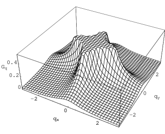
Figure 1: Generic ferroelectric propagator Eq. (10) in the static limit $\varpi=0$ with cubic symmetry and large anisotropy; $q_{z}=0$, $r=0$, $f=5.0$, $\Lambda=\pi$.

III Propagator and modes

Eq. (II) and Eq. (II) define a model for the phase transition in a ferroelectric near a quantum critical point. In the absence of nonlinearities, the Heisenberg order parameter correlation function $G^{0}_{\alpha\beta}=\langle\phi_{\alpha}\phi_{\beta}\rangle_{0}$ is Fisher73

$$G_{\alpha\beta}^{0} ={1\over r_{\alpha}+\varpi^{2}+q^{2}+f_{\alpha}q_{\alpha}^{2}}$$ (8a)

$$\times\left(\delta_{\alpha\beta}-{(g-hq^{2})q_{\alpha}q_{\beta}\over\left[q^{2}+(g-hq^{2})Q\right][r_{\beta}+\varpi^{2}+q^{2}+f_{\beta}q_{\beta}^{2}]}\right)$$

$$Q =\sum_{\gamma}{q_{\gamma}^{2}\over r_{\gamma}+\varpi^{2}+q^{2}+f_{\gamma}q_{\gamma}^{2}}$$ (8b)

Here $\varpi=2n\pi(T/E_{0})$ is a dimensionless bosonic Matsubara frequency, and in our conventions $G$ is dimensionless.

The nature of the modes defined by the poles of Eq. (8a) can be best understood by considering the polarization of the ferroelectric fluctuation vector ${\bm{\phi}}$. For every ${\bf q}$ there are $d-1$ transverse and one longitudinal polarizations, all orthogonal to each other. The longitudinal mode is always stiff with $\varpi_{\parallel}={\mathcal{O}}(g)$, and $h$ only enters the dispersion of the longitudinal mode; both $g$ and $h$ are irrelevant to the critical behavior. The remaining $d-1$ modes are soft and in the case of cubic symmetry have the general dispersion

$$\varpi^{2}_{\lambda}(q)=r_{\lambda}+q^{2}\left[1+fA_{\lambda}(\Omega_{q})\right]$$ (9)

where $\Omega_{q}$ is the set of angles defining the direction of ${\bf q}$ and $A_{\lambda}$ are lengthy expressions derived from Eq. (8a). Eq. (9) includes all modes with the convention $r_{\perp}=r$, $r_{\parallel}=r+g$. For all ${\bf q}$ such that the polarization of a transverse mode points along a crystal axis the respective dispersion softens additionally ($A_{\lambda}(\Omega_{q})=0$) if $f>0$. The effect of $f$ is most easily seen by setting $q_{z}=0$ and considering only the $XY$ block. The resulting transverse mode propagator

$$G(\varpi,q)=\left(r+\varpi^{2}+q_{x}^{2}+q_{y}^{2}+2f{q_{x}^{2}q_{y}^{2}\over q_{x}^{2}+q_{y}^{2}}\right)^{-1}$$ (10)

is shown in Fig. (1). The dipolar anisotropy ($f$) leads to ridges suggestive of quasi one dimensional behavior.

	$\hbar c$ [$m$eV-Å]	$E_{0}$ [$m$eV]	$f$	$u$	$v$
BaTiO3	6.36	5.00	4.7	1.25	0.68
PbTiO3	6.79	5.37	1.1	0.26	-0.09

Table 1: Numerical values of the parameters used in the action Eq. (II). The values for $u$ and $v$ are initial conditions for the RG flow of the two interaction constants in Eq. (II).

IV Interaction renormalization

Figure 2: One loop diagrams for the renormalization of (a) the quartic interaction $u$ and (b) the masses $r_{\alpha}$.

We obtain the parameters $c$, $r_{\alpha}$, $f_{\alpha}$, $g$ and $h$ in Eq. (II) by fitting the poles of Eq. (8a) to first-principles phonon dispersion curves such as those in Ref. Ghosez99 . We fit the numerically calculated mode frequencies near the zone center to the modes predicted by Eq. (8a) along crystal symmetry directions. The soft modes’ speed $c$ and mass $r(T=0)$ at the lattice constants used in Ref. Ghosez99 (ambient pressure) are readily obtained by fitting the dispersions along (100) to $\omega=c\sqrt{r/a^{2}}+(1/2)c\sqrt{r/a^{2}}(q/a)^{2}+{\mathcal{O}}(q^{4})$. The anisotropy parameter $f$ is obtained from direct ratios of the curvature of the dispersion along (110) and (111).

The size of the interaction constants $u$ and $v$ can be estimated from first-principles variational studies of a Landau free energy of the system Vanderbilt94 $E({\bf w})=\kappa{\bf w}^{2}+\alpha^{\prime}{\bf w}^{4}+\gamma^{\prime}\sum_{\alpha>\beta}w_{\alpha}^{2}w_{\beta}^{2}$ where $E({\bf w})$ is the free energy per unit cell and ${\bf w}$ is a soft mode lattice displacement. The parameters $\alpha^{\prime}$ and $\gamma^{\prime}$ (Table V in Vanderbilt94 ) studied by these authors are related to $u$ and $v_{\alpha}=v$ in Eq. (II) by $u=(\alpha^{\prime}+\gamma^{\prime}/2)(r/\kappa)^{2}E_{0}$ and $v=-(\gamma^{\prime}/2)(r/\kappa)^{2}E_{0}$. For BaTiO₃ and PbTiO₃ (which have cubic symmetry so $v_{\alpha}=v$ and $f_{\alpha}=f$) we find the results listed in Table 1.

We now study the relevance of quartic interactions in the vicinity of the critical point. The one-loop correction to $u$ and $v$ is given generically by the diagram in Fig. (2a) and the respective renormalization equation Aharony73 is given by

$$\sum_{\alpha\beta}u_{\alpha\beta}^{l+1}\phi^{\alpha}\phi^{\alpha}\phi^{\beta}\phi^{\beta}=\zeta_{l}^{4}b^{-3(d+z)}\Big{[}\sum_{\alpha\beta}u_{\alpha\beta}^{l}\phi^{\alpha}\phi^{\alpha}\phi^{\beta}\phi^{\beta}\\ -4\sum_{\alpha\beta\gamma\delta}u_{\alpha\gamma}^{l}u_{\beta\delta}^{l}\big{(}w_{\gamma\delta\gamma\delta}\phi^{\alpha}\phi^{\alpha}\phi^{\beta}\phi^{\beta}\\ +4w_{\gamma\beta\gamma\delta}\phi^{\alpha}\phi^{\alpha}\phi^{\beta}\phi^{\delta}+4w_{\alpha\beta\gamma\delta}\phi^{\alpha}\phi^{\beta}\phi^{\gamma}\phi^{\delta}\big{)}\Big{]}$$ (11)

where $u_{\alpha\beta}=u+v\delta_{\alpha\beta}$, the external momentum integrations are omitted for brevity, and $w_{\alpha\beta\gamma\delta}$ are the one-loop integrals over fast modes

$$w_{\alpha\beta\gamma\delta}=T\sum_{\varpi_{n}}\int{{\rm d}^{d}q\over(2\pi)^{d}}G^{0}_{\alpha\beta}(\varpi,q)G^{0}_{\gamma\delta}(\varpi,q).$$ (12)

In Eq. (11) $\zeta_{l}=b^{1+d/2}$ is the field renormalization when the fast modes in the shell $\Lambda/b<q<\Lambda$ are integrated out. The diagrammatic version of Eq. (11) is shown in Fig. (3).

Figure 3: Renormalization diagrams to tree and one-loop order for the anisotropic interaction parameter $u_{\alpha\beta}=u+v\delta_{\alpha\beta}$ in Eq. (II). This is the diagrammatic representation of Eq. (11).

In $d=3$ the system is in its marginal dimension and the prefactor in Eq. (11) is $\zeta_{l}^{4}b^{-3(d+z)}$ so that the leading interaction renormalization is quadratic. The generic form of the renormalization equations is

$$-\delta u\sim u^{2}\int_{-\infty}^{\infty}{{\rm d}\varpi\over 2\pi}\int^{\pi}{{\rm d}^{d}q\over(2\pi)^{d}}G^{2}(\varpi,q)\coth{\varpi\over 2T},$$ (13)

where $G$ is a soft eigenmode of the Gaussian ferroelectric propagator. We first consider the simplest case of isotropic interactions ($v_{\alpha}=0$) in an isotropic medium ($f_{\alpha}=0$, $r_{\alpha}=r$) in the low temperature limit, and we also let $h=0$ for simplicity. As explained above, the correlation function Eq. (8a) then has a Heisenberg-like rotationally invariant form with $d-1$ soft eigenmodes $G^{-1}=r+\varpi^{2}+q^{2}=r+Q^{2}$ and one stiff (non-critical) eigenmode $G^{-1}=r+Q^{2}+g$. Including only the soft eigenmodes in Eq. (13) the recursion relation for $u$ is respectively

$$-\delta u\sim\int^{\pi}{u^{2}Q^{d}\over(r+Q^{2})^{2}}dQ\sim u^{2}\left\{\begin{array}[]{lc}\log 1/r,&\quad d=3\\ 1/\sqrt{r},&\quad d=2\\ 1/r,&\quad d=1.\end{array}\right.$$ (14)

Eq. (14) shows that upper critical dimension of a Heisenberg isotropic quantum critical ferroelectric system is $d_{c}=3$.

For a uniaxial (Ising-like) ferroelectric there is a preferred ‘easy axis’ for the orientation of ${\bm{\phi}}$ which brings about a further increase in effective dimensionality Fisher73 . The respective correlation function has the form $G(\varpi,q)=(r+\varpi^{2}+q^{2}+g_{I}q_{z}^{2}/q^{2})^{-1}$ which gives for $\delta u$

$$-\delta u \sim u^{2}\int{\rm d}\varpi\int{\rm d}q\int{q^{d-1}{\rm d}\cos\theta\over(r+\varpi^{2}+q^{2}+g_{I}\cos^{2}\theta)^{2}}$$ (15)

$$\sim {u^{2}\over g_{I}^{1/2}}\int^{\pi}{Q^{d+1}{\rm d}Q\over(r+Q^{2})^{2}}\sim{u^{2}\over g_{I}^{1/2}}\left\{\begin{array}[]{lc}r^{1/2},&\qquad d=3\\ \log 1/r,&\qquad d=2.\end{array}\right.$$ (18)

Thus the upper critical dimension of an Ising isotropic quantum critical ferroelectric system is reduced to $d_{c}=2$. In the case of a preferred ‘easy plane’ of polarization the propagator has the two eigenmodes $G=(r+\varpi^{2}+q^{2})^{-1}$ and $G=(r+\varpi^{2}+q^{2}+g\sin^{2}\theta)^{-1}$ so that the $XY$ -model and Heisenberg ferroelectrics have identical coupling renormalizations which is due to the existence of the same soft mode in both cases.

We now study the possibility that the quasi one dimensional behavior associated with $f>>1$ may modify the criticality. We illustrate the issues using the notationally simpler $d=2$, $g\to\infty$ case, and have verified that our results hold in $d=3$ also. From Fig. (2a) and Eq. (10) we obtain, after integration over $\varpi$ and the magnitude of $q$

$$-\delta u = \left({u\over 4\pi}\right)^{2}\int_{0}^{2\pi}{{\rm d}\varphi\over 1+(f/2)\sin^{2}2\varphi}$$

$$\times\left[{1\over\sqrt{r}}-{1\over\sqrt{r+\Lambda^{2}(1+(f/2)\sin^{2}2\varphi)}}\right]$$

$$\approx {u^{2}\over 8\pi^{2}\sqrt{2fr}}\left[\pi-2\tan^{-1}{\sqrt{r}\over\Lambda}\right]\sim\left\{\begin{array}[]{lr}r^{-1/2},&r<\Lambda^{2}\\ \Lambda/r,&r>\Lambda^{2}.\end{array}\right.$$ (22)

In the second, approximate equality we have taken the large $f$ limit. We see from this that the quasi one dimensional structure does not affect the degree of divergence as $r\to 0$; indeed $f$ only affects prefactors and not the scale $\Lambda^{2}$ to which $r$ should be compared. To summarize, a mean-field treatment of the model Eq. (II) should be qualitatively correct except in the case of a $d=2$ $XY$ ferroelectric, and we exclude this case henceforth.

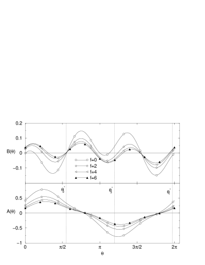
Figure 4: Coefficients of the angular and radial part of the interaction renormalization coefficient Eq. (25) at $T=0$. The stable roots of $B(\theta)$ which determine the nature of the fixed points are marked by vertical dotted lines.

We further study the fixed points of Eq. (11) in its full anisotropic form. The Gaussian propagator Eq. (8a) in the strong dipole interaction limit $g\to\infty$ is

$$G^{0}_{\alpha\beta}(\varpi,q)={1\over r+\varpi^{2}+q^{2}+fq_{\alpha}^{2}}\\ \times\left(\delta_{\alpha\beta}-{q_{\alpha}q_{\beta}\over Q\left(r+\varpi^{2}+q^{2}+fq_{\beta}^{2}\right)}\right)$$ (23)

where $Q$ is defined in Eq. (8b). With the use of cubic symmetry, the possible combinations of $w_{\alpha\beta\gamma\delta}$ are reduced to

$$w_{\alpha\beta\gamma\delta}=\left[\left(A_{1}-A_{2}\right)\delta_{\alpha\gamma}+A_{2}\right]\delta_{\alpha\beta}\delta_{\gamma\delta}\\ +A_{3}\left(1-\delta_{\alpha\beta}\right)\left(\delta_{\alpha\gamma}\delta_{\beta\delta}+\delta_{\alpha\delta}\delta_{\beta\gamma}\right)$$ (24)

The $f$- and $T$-dependent integrals $A_{1,2,3}$ are calculated in the Appendix. Substituting Eq. (24) in Eq. (11) yields coupled nonlinear renormalization equations for $u$ and $v$, similar to those written by Aharony and Fisher Aharony73 for the classical case (but note that Aharony and Fisher expanded the coefficients $A_{i}$ about the limit of small anisotropy whereas we retain their full $f$ dependence). The stability of the Gaussian fixed point $u=v=0$ is most transparently analysed using polar coordinates in the $(u,v)$ plane: $u=\rho\cos\theta$ and $v=\rho\sin\theta$. The renormalization equations for $u$ and $v$ then become

$${{\rm d}\rho\over{\rm d}\ln\Lambda} =-A(\theta,T)\rho^{2}$$ (25a)

$${{\rm d}\theta\over{\rm d}\ln\Lambda} =-B(\theta,T)\rho$$ (25b)

The $\theta$- and $T$-dependent coefficients $A$ and $B$ are given in the Appendix (Eq. (A7)), and their $T=0$ limit is plotted in Fig. (4). These coefficients are to be evaluated at the running temperature $T(\Lambda)=T_{\text{phys}}e^{\ln\Lambda}$ and are derived on the assumption that the physics is dominated by the (Gaussian) quantum critical point; in other words, on the assumption that control parameter $r$, interaction amplitude $\rho$ and temperature are not too large. In particular, the model exhibits a pase transition at a temperature $T_{c}(r)$ discussed in detail below. At temperatures sufficiently near to $T_{c}(r)$ a crossover to physics controlled by a classical, non-Gaussian critical point will occur and the theory used here ceases to apply. To estimate the region of applicability of the equations presented here we follow Millis93 , noting first that the breakdown of the quantum critical theory will occur in the classical region $T(\Lambda)>\Lambda$. In this regime the relevant dimensionless interaction amplitude is $\rho_{\text{classical}}=T(\Lambda)\rho(\Lambda)/\Lambda$ and Eq. (25a) predicts the classical fixed point $\rho^{\star}_{\text{classical}}=\lim_{T\to\infty}T/(\Lambda A(\theta,T))$. We find $\rho^{\star}_{\text{classical}}=\{1.25318,1.47604\}$ for the two fixed lines $\theta_{1}^{\star}$, $\theta_{2}^{\star}$ respectively, shown in Fig. (5), and for $f=1.1$. The $f$-dependence of $\rho^{\star}_{\text{classical}}$ can be be summarized by the linear fits $\rho^{\star}_{\text{classicl}}\approx 1.16+0.11f$ for the $\theta_{1}^{\star}$ fixed line, and $\rho^{\star}_{\text{classicl}}\approx 0.48+0.77f$ for the $\theta_{2}^{\star}$ fixed line. As an estimate of the range of validity of the scaling equations, we argue they apply for $\rho_{\text{classical}}\lesssim(1/2)\rho^{\star}_{\text{classical}}$, which corresponds to the $3D$ Ginzburg criterion $\rho_{\text{classical}}/r^{1/2}_{\text{classical}}\sim 1$.

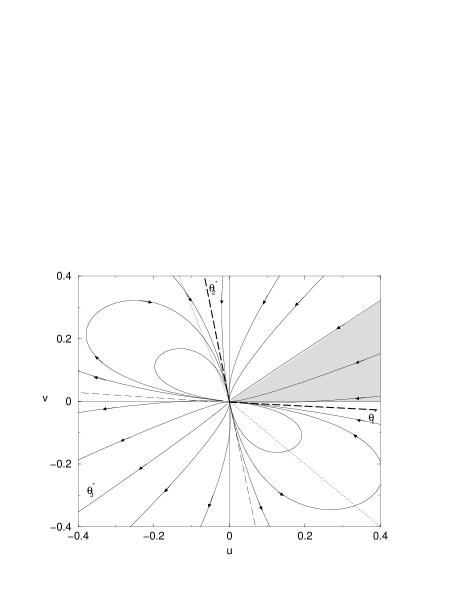
Figure 5: Phase portrait for Eq. (25) with $f=1.1$. The heavy dashed lines indicate the $u/v$ ratios corresponding to stable fixed points of Eq. (25); their continuations (light dashed lines) mark the boundaries of the unstable region where $\rho$ flows to large values. The dotted lines mark the mean-field stability boundaries Eq. (7). The shaded region indicates initial conditions ($u_{0},v_{0}$) which start with Ising-like polarization orientation but eventually flow to the fixed line $\theta^{\star}_{1}$ with nearly Heisenberg polarization orientation along (111).

We wish to study the stability of the fixed point $\rho=0$ in Eq. (25). The solutions of Eq. (25) asymptotically approach the fixed point along ‘invariant lines’ $\dot{\theta}=0$ given by the stable roots $\theta^{\star}$ of $B(\theta,T)$ (Eq. (A7b)). Respectively, Eq. (25) has a stable fixed point $\rho\to 0$ if $A(\theta^{\star},T)>0$. The functions $A(\theta)$ and $B(\theta)$ are shown in Fig. (4) for several values of the anisotropy $f$. It is seen that there are three ‘invariant lines’ of which $\theta^{\star}_{3}$ (the middle in Fig. (4)) is unstable ($A(\theta^{\star}_{3})<0$). The two stable solutions are $\theta^{\star}_{1}\lesssim 0$ corresponding to a nearly Heisenberg fixed point $|u|>>v$; $u<0$, and $\theta^{\star}_{2}\gtrsim\pi/2$ corresponding to an Ising-like fixed point $v>>|u|$, $u<0$. The dependence of $\theta^{\star}_{1,2}$ on $f$ is weak and does not change the qualitative behavior. The nature of the ‘fixed line’ solutions is most clearly seen in Fig. (5) which shows the phase portrait of Eq. (25). The stable fixed lines $\theta^{\star}_{1,2}$ are shown by heavy dashed lines. Above and to the right of the light dashed lines the flows are stable ($\rho\to 0$); below and to the left, unstable ($\rho\to\infty$). The region of stability found in the RG analysis is wider than that found in the mean field approximation (Eq. (7) shown in Fig. (5) as light dotted lines). The physical content of the two fixed lines $\theta^{\star}_{1,2}$ is different: $\theta^{\star}_{1}$ corresponds to a nearly isotropic system with polarization along (111) but a relatively weak barrier against polarization reorientation ($v/|u|\sim 0.15$, but weakly $f$-dependent), whereas $\theta^{\star}_{2}$ corresponds to a strongly anisotropic system with polarization along (100) and a barrier of relative order unity. It is seen in Fig. (5) that there exists a range of initial conditions in the shaded wedge between the $v=0$ axis and the separatrix in the first quadrant, which start with initial values $v_{0}>0$ favoring Ising symmetry but eventually flow to the $\theta^{\star}_{1}$ fixed line with $v<0$ and Heisenberg polarization symmetry.

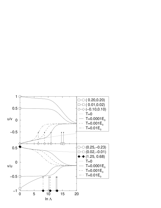
Figure 6: The solutions of Eq. (25) for $f=1.1$ plotted for several different initial conditions. Selected trajectories are shown for several temperatures. The trajectories converge into one of two ‘fixed lines’ also seen in Fig. (5). The top and bottom panels show trajectories converging to $\theta_{2}^{\star}$ and $\theta_{2}^{\star}$ respectively. The two panels are shown with inverted interaction constant ratios relative to each other to capture the significant features of the fixed line approach in each case. The arrows mark the quantum – classical crossover $\rho_{\text{classical}}\sim\rho^{\star}_{\text{classical}}$. Trajectories that undergo polarization reorientation are marked with filled symbols.

We see that the ratio and even the sign of $u/v$ may change under renormalization. In particular, for initial $u>0$, $v>0$ and $u/v$ less than an ($f$-dependent) critical value of the order of unity, the sign of $v$ changes under renormalization, corresponding to a predicted change in the polarization direction as criticality is approached. Unfortunately, the logarithmic nature of the scaling, combined with the numerically small value of $B(\theta,T)$ and the factor of $\rho$ in Eq. (25b) means that at $T=0$ one must approach criticality extraordinarily closely to observe the effect. The scaling turns out to be more rapid in the classical regime $T(\Lambda)>\Lambda$, but as noted above our analysis cannot be extended too far into this regime before the equations break down.

To further illustrate this point and to study how “soon” in RG time this change of ordered state orientation occurs, and each fixed line is reached, we show in Fig. (6) the evolution of the ratio of the two interaction constants along typical trajectories in Fig. (5). It is seen that the trajectories reach their ‘fixed line’ regime relatively late with long temperature dependent transients sensitive to initial conditions. Trajectories that start with Ising symmetry $v_{0}>0$ and ultimately flow to a Heisenberg fixed line with $v<0$ are marked with filled symbols. For example, the initial conditions for BaTiO₃ are within the shaded range in Fig. (5), and the sign reversal is expected to occur for $T=0.0001E_{0}$ at $\ln\Lambda\sim 15$.

The phase portrait Fig. (5) changes only quantitatively with increased anisotropy, e.g. $f=5$: the closed loop trajectories shrink towards the origin as higher anisotropy reduces both interactions $u$ and $v$ (Eq. (A3)), and the slope of the fixed lines changes according to the $\theta$-roots shown in Fig. (4).

V Free energy, specific heat and mass renormalization

Within the Gaussian approximation the free energy per unit cell of the system is given by

$$F=\sum_{\lambda}\int_{q}\left[{1\over 2}E_{0}\varpi_{\lambda}(q)+T\ln\left(1-e^{-\varpi_{\lambda}(q)E_{0}/T}\right)\right]$$ (26)

where $\varpi_{\lambda}$ are the poles of Eq. (8a). The specific heat can be obtained directly from this expression as

$$C=-T{\partial^{2}F\over\partial T^{2}}=\sum_{\lambda}\int{{\rm d}^{d}q\over(2\pi)^{d}}{\left[\varpi_{\lambda}(q)E_{0}/2T\right]^{2}\over\sinh^{2}\left[\varpi_{\lambda}(q)E_{0}/2T\right]}$$ (27)

Using the general form of the eigenmodes in a cubic Heisenberg system with anisotropy Eq. (9) and the isotropic Ising mode $\varpi^{2}(q)=r+q^{2}+g_{I}\cos^{2}\theta$ the asymptotic low-temperature behavior of the specific heat is

$$C_{H} = \sum_{\lambda=1}^{2}\int{{\rm d}\Omega_{q}\over\pi^{3}}{(T/E_{0})^{3}\over\left[1+fA_{\lambda}(\Omega_{q})\right]^{3/2}}\int_{0}^{\infty}{x^{2}\left(\kappa+x^{2}\right){\rm d}x\over\sinh^{2}\sqrt{\kappa+x^{2}}}$$

$$C_{I} = {3\over\pi\sqrt{g_{I}}}\left({T\over E_{0}}\right)^{4}\int_{0}^{\infty}{t(\kappa+t)\over\sinh^{2}\sqrt{\kappa+t}}{\rm d}t$$ (28)

where $H$ and $I$ refer to Heisenberg and Ising respectively and $\kappa=(E_{0}/2T)^{2}r$. As is seen from Eq. (28) in the low-temperature limit the anisotropy $f$ enters only as a multiplicative factor in a $f=0$ expression for the specific heat. The specific heats of a $d=3$ Heisenberg model are shown in Fig. (7) for $r=0$ (main figure) and away from the critical point (inset). We see that except in the unrealistically strong ($f>100$) case the only crossover visible is from the quantal ($C\sim T^{3}$) to classical ($C\sim$ const) behavior as $T$ is increased through the largest zone boundary phonon frequency (shown by arrows in Fig. (7). The crossover from Heisenberg to Ising symmetry is shown in inset b) of Fig. (7) for a set of Ising interaction strengths $g_{I}$.

Figure 7: Main figure: critical point specific heat per unit cell to Gaussian order in units of $k_{B}$ for a $d=3$ Heisenberg model for a set of anisotropy parameters $f$. The vertical arrows mark the points $t=\sqrt{2+f}$ for each respective curve. Inset: a) the $r$-dependence of $C(t)$ for $f=5$; b) Heisenberg to Ising crossover in specific heat, for $f=0$.

Figure 8: Pressure dependence of the ferroelectric critical temperature for the following cases: an Ising model with $g_{I}=10$ and $v_{0}=1$; PbTiO₃ and BaTiO₃ with parameters in Table 1; an isotropic model with $f=0$, $u_{0}=2$.

Finally we study the pressure dependence of the transition temperature. The mass flow equation is given by

$${\rm d}r=2r(\Lambda)\ {\rm d}\ln\Lambda+{\rm d}R(\Lambda)$$ (29)

where ${\rm d}R(\Lambda)$ represents the one loop mass correction Fig. (2b). It is possible to express this diagram in terms of an invariant of Eq. (8a)

$${\rm d}R(\Lambda)=\displaystyle{4\over d}[(d+2)u(\Lambda)+3v(\Lambda)]T\sum_{\varpi_{n}}^{\prime}\int^{\prime}{{\rm d}^{d}q\over(2\pi)^{d}}\ \text{Tr}{\bf G^{0}}$$ (30)

where the $q$-integration and Matsubara frequency summation are performed in narrow shells of width ${\rm d}\Lambda$ for each variable while the other one is held fixed at the bandwidth cutoff, e.g. $\varpi_{n}\in[\Lambda,\Lambda+{\rm d}\Lambda]$ while $q=\Lambda$, and $q\in[\Lambda,\Lambda+{\rm d}\Lambda]$ while $\varpi_{n}=\Lambda$. The trace in Eq. (30) is over the propagator eigenvalues Eq. (A1b). Using the identity

$$T\sum_{\varpi_{n}}{1\over\varpi_{n}^{2}+\omega_{\lambda}^{2}(q)}=\int_{0}^{\infty}{{\rm d}\omega\over 2\omega}\coth{\omega\over 2T}\delta\left(\omega-\omega_{\lambda}(q)\right)$$

we obtain the solution of Eq. (29) for $d=3$ in explicit form

$$r(\Lambda)= e^{2\ln\Lambda}\left\{r_{0}+\int_{0}^{\ln\Lambda}{\rm d}\ln\Lambda^{\prime}e^{-2\ln\Lambda^{\prime}}4\left[{5\over 3}u(\Lambda^{\prime})+v(\Lambda^{\prime})\right]\right.$$

$$\times{\Lambda^{2}\over 16\pi^{3}}\sum_{\lambda}\int{\rm d}\Omega{1\over\sqrt{1+fA_{\lambda}(\Omega)}}$$ (31)

$$\qquad\times\left.\left[\coth{\Lambda\sqrt{1+fA_{\lambda}(\Omega)}\over 2Te^{\ln\Lambda^{\prime}}}+{\coth\Lambda/2Te^{\ln\Lambda^{\prime}}\over 1+fA_{\lambda}(\Omega)}\right]\right\}$$

Here $r_{0}$ is the initial condition for the mass; $u(\Lambda)$ and $v(\Lambda)$ are the solutions to Eq. (25); $A_{\lambda}(\Omega)$ are the angular dependent anisotropic factors of the dispersion from Eq. (9), and $T(\Lambda)=Te^{\ln\Lambda}$ is the flowing temperature while $T$ is the real physical temperature. We find $T_{c}$ from the requirement that at the critical temperature the mass flows to zero: $r(\Lambda\to\infty)$. The quantum critical control parameter (which in experimental realizations corresponds to e.g. hydrostatic pressure, doping, etc.) is $r-r_{c}=r_{0}(T)-r_{0}(T=0)$. We point out that since a $3D$ ferroelectric is above its upper critical dimension we obtain a qualitatively identical phase boundary if we simply use the initial conditions $u_{0}$ and $v_{0}$ for the interaction constants in Eq. (V). In that case $T_{c}(r-r_{c})$ can be obtain from the simpler expression

$$|r-r_{c}|=\sum_{\lambda}\int^{\pi}{d^{d}q\over(2\pi)^{d}}{{4\over d}\left[(d+2)u_{0}+3v_{0}\right]\over\varpi_{\lambda}(q)\left[\exp\left({E_{0}\over T_{c}}\varpi_{\lambda}\right)-1\right]}$$ (32)

The phase boundary $T_{c}(r-r_{c})$ obtained from Eq. (32) is shown in Fig. (8) for four representative sets of parameters. All curves in Fig. (8) except Ising behave as $T_{c}\sim|r-r_{c}|^{1/2}$ near $r_{c}$; the Ising behavior is $T_{c}\sim|r-r_{c}|^{1/3}$. All curves cross over to $T_{c}\sim|r-r_{c}|$ as $T$ is increased through the softest zone boundary phonon frequency $E_{0}$.

We briefly consider the effect of a small density of free carriers characterized by an inter-carrier spacing $L_{F}$ and a diffusion constant $D_{F}$. At length scales longer than $L_{F}$ and frequency scales lower than $\omega_{F}=D_{F}/L_{F}^{2}$, these carriers will screen the interaction on the scale $L_{F}$ and overdamp the dynamics. The details of the crossover depend on the ratio $D_{F}/cL_{F}$. If $D_{F}/cL_{F}>>1$, then there is a two-stage crossover: as the scale is decreased, first the dynamics becomes overdamped and then subsequently the characteristic length scale passes through the screening length and the interaction becomes effectively short ranged. On the other hand, if $D_{F}/cL_{F}<<1$, then screening and overdamping occur at the same scale. Further studies of this crossover will be presented elsewhere.

All cases except for $2d$ $XY$ symmetry are above the upper critical dimension enabling a controlled treatment. Lattice-induced anisotropies arising from the dipolar interaction are not small in real materials, and lead e.g. to strong “quasi one-dimensional” effects in the phonon spectrum (cf Fig. 1). However, we showed that for systems above the upper critical dimension the effect on the critical behavior is unimportant; only for unrealistically strong anisotropies $f>100$ is an intermediate quasi one-dimensional regime visible in the specific heat. A change of polarization direction under scaling is suggested for BaTiO₃ near $T_{c}(p)$ and for $p$ sufficiently close to the critical pressure at which $T_{c}\to 0$ (although the scaling equations break down at approximately the scale of the anisotropy change). We have presented exact results, in physical units, for the phase boundary and specific heat. For PbTiO₃ and BaTiO₃ quantum critical effects are dominant for $T<50$K if the materials are tuned by pressure to the quantum critical point.

Acknowledgements: We thank K. M. Rabe for helpful conversations and NSF DMR 00081075 and the University of Maryland – Rutgers MRSEC for support.

VI Appendix

We calculate the one-loop diagrams Eq. (12) by using a diagonal representation for the Gaussian propagator achieved through the rotation matrix ${\bf R}$

$$G^{0}_{\alpha\beta} =R_{\alpha\sigma}g_{\sigma}(\varpi_{n},q)R^{-1}_{\sigma\beta}$$ (A1a)

where

$$g_{\sigma}(\varpi_{n},q) ={1\over\varpi_{n}^{2}+\omega_{\sigma}^{2}(q)}={1\over\varpi_{n}^{2}+r_{\sigma}+q^{2}(1+fA_{\sigma}(\theta,\varphi))}$$ (A1b)

The one-loop integrals then become

$$\begin{split}w_{\alpha\beta\gamma\delta}&=T\sum_{\varpi_{n}}\int{{\rm d}^{d}q\over(2\pi)^{d}}\sum_{\mu\nu}R_{\alpha\mu}{1\over\varpi_{n}^{2}+\omega_{\mu}^{2}(q)}R^{-1}_{\mu\beta}R_{\gamma\nu}{1\over\varpi_{n}^{2}+\omega_{\nu}^{2}(q)}R^{-1}_{\nu\delta}\\ &=i\int_{0}^{\infty}{{\rm d}\omega\over 2\pi}\int{{\rm d}^{d}q\over(2\pi)^{d}}\sum_{\mu\nu}R_{\alpha\mu}R^{-1}_{\mu\beta}R_{\gamma\nu}R^{-1}_{\nu\delta}\Im{1\over\left[\omega^{2}+\omega_{\mu}^{2}(q)\right]\left[\omega^{2}+\omega_{\nu}^{2}(q)\right]}\coth{\omega\over 2T}\\ \end{split}$$ (A2)

We perform the integration over the magnitude of $q$ in $d=3$ and obtain the remaining integrals over angles only, which we then calculate numerically

$$w_{\alpha\beta\gamma\delta}=\begin{cases}\begin{split}{1\over 16\pi^{3}}{{\rm d}\Lambda\over\Lambda}\sum_{\mu\nu}&\int{\rm d}\Omega_{q}R_{\alpha\mu}R^{-1}_{\mu\beta}R_{\gamma\nu}R^{-1}_{\nu\delta}{1\over f\left[A_{\nu}(\Omega_{q})-A_{\mu}(\Omega_{q})\right]}\\ &\times\left({\coth\displaystyle{\Lambda\sqrt{1+fA_{\mu}}\over 2T}+\coth\displaystyle{\Lambda\over 2T}\over\sqrt{1+fA_{\mu}}}-{\coth\displaystyle{\Lambda\sqrt{1+fA_{\nu}}\over 2T}+\coth\displaystyle{\Lambda\over 2T}\over\sqrt{1+fA_{\nu}}}\right)\end{split}&\text{for \ }A_{\mu}(\Omega_{q})\neq A_{\nu}(\Omega_{q})\\ \begin{split}{1\over 16\pi^{3}}{{\rm d}\Lambda\over\Lambda}\sum_{\mu\nu}&\int{\rm d}\Omega_{q}R_{\alpha\mu}R^{-1}_{\mu\beta}R_{\gamma\nu}R^{-1}_{\nu\delta}{1\over 2\left[1+fA_{\mu}(\Omega_{q})\right]^{3/2}}\\ &\times\left[\coth\displaystyle{\Lambda\sqrt{1+fA_{\mu}}\over 2T}\left(1+{\displaystyle{\Lambda\over T}\sqrt{1+fA_{\mu}(\Omega_{q})}\over\sinh\displaystyle{\Lambda\over T}\sqrt{1+fA_{\mu}(\Omega_{q})}}\right)+\coth\displaystyle{\Lambda\over 2T}\right]\end{split}&\text{for \ }A_{\mu}(\Omega_{q})=A_{\nu}(\Omega_{q})\end{cases}$$ (A3)

The isotropic case $f=0$ is described by the second expression in Eq. (A3). For numerical calculations Eq. (A3) is more conveniently written as

$$w_{\alpha\beta\gamma\delta}=\begin{cases}\begin{split}{\Lambda\over 16\pi^{3}}{\rm d}\Lambda\sum_{\mu\nu}&\int{\rm d}\Omega_{q}R_{\alpha\mu}R_{\beta\mu}R_{\gamma\nu}R_{\delta\nu}{g_{\mu}g_{\nu}\over\sqrt{g_{\mu}}+\sqrt{g_{\nu}}}\\ &\times\left({\sqrt{g_{\mu}}\coth\Lambda/(2T\sqrt{g_{\mu}})-\sqrt{g_{\nu}}\coth\Lambda/(2T\sqrt{g_{\nu}})\over\sqrt{g_{\mu}}-\sqrt{g_{\nu}}}+\coth{\Lambda\over 2T}\right)\end{split}&\text{for \ }g_{\mu}\neq g_{\nu}\\ \begin{split}{\Lambda\over 16\pi^{3}}{\rm d}\Lambda\sum_{\mu\nu}&\int{\rm d}\Omega_{q}R_{\alpha\mu}R_{\beta\mu}R_{\gamma\nu}R_{\delta\nu}\left({1\over 2}g_{\mu}^{3/2}\right)\\ &\times\left[\coth\displaystyle{\Lambda\over 2T\sqrt{g_{\mu}}}\left(1+{\Lambda/(T\sqrt{g_{\mu}})\over\sinh\Lambda/(T\sqrt{g_{\mu}})}\right)+\coth\displaystyle{\Lambda\over 2T}\right]\end{split}&\text{for \ }g_{\mu}=g_{\nu}\end{cases}$$ (A4)

Here $R_{\alpha\mu}$ is a matrix whose columns are the $\mu$-th eigenvector and $g_{\mu}=\Lambda^{2}[1+fA_{\mu}(\Omega_{q})]$ is the $\mu$-th eigenvalue of Eq. (23) both evaluated at $\varpi=0$; $r=0$; $q=\Lambda$, and both having an implicit angular dependence. At low temperatures $T<\Lambda$ Eq. (A4) reduces to

$$w_{\alpha\beta\gamma\delta}={\Lambda\over 8\pi^{3}}{\rm d}\Lambda\sum_{\mu\nu}\int{\rm d}\Omega_{q}R_{\alpha\mu}R_{\beta\mu}R_{\gamma\nu}R_{\delta\nu}{g_{\mu}g_{\nu}\over\sqrt{g_{\mu}}+\sqrt{g_{\nu}}}$$ (A5)

The cubic-symmetric integrals $A_{1,2,3}$ appearing in Eq. (24) are defined as

$$A_{1}(b) =T\sum_{\varpi_{n}}\int{{\rm d}^{d}q\over(2\pi)^{d}}\ \left(G^{zz}\right)^{2}=w_{zzzz}$$ (A6a)

$$A_{2}(b) =T\sum_{\varpi_{n}}\int{{\rm d}^{d}q\over(2\pi)^{d}}\ G^{xx}G^{yy}=w_{xxyy}$$ (A6b)

$$A_{3}(b) =T\sum_{\varpi_{n}}\int{{\rm d}^{d}q\over(2\pi)^{d}}\ \left(G^{xy}\right)^{2}=w_{xyxy}$$ (A6c)

and are calculated from Eq. (A4) numerically.

The angle-dependence of the $\rho$ and $\theta$ derivatives in Eq. (25) is given by

$$A(\theta,T)= \ a_{1}\cos^{3}\theta+c_{2}\sin^{3}\theta$$ (A7a)

$$+\sin\theta\cos\theta\big{[}(b_{1}+a_{2})\cos\theta+(c_{1}+b_{2})\sin\theta\big{]}$$

$$B(\theta,T)= \ a_{2}\cos^{3}\theta-c_{1}\sin^{3}\theta$$ (A7b)

$$+\sin\theta\cos\theta\big{[}(b_{2}-a_{1})\cos\theta+(c_{2}-b_{1})\sin\theta\big{]}$$

where

$$a_{1} =4(3A_{1}+4A_{2}+14A_{3}) a_{2} =16(A_{1}-A_{2}-2A_{3})$$

$$b_{1} =8(5A_{1}+16A_{3}) b_{2} =48(A_{1}-A_{3})$$

$$c_{1} =36A_{3} c_{2} =36(A_{1}-A_{3})$$

References

- (1) Lines M.E. and Glass A.M., Principles and Applications of Ferroelectrics and Related Materials (Oxford University Press, Oxford 1977)
- (2) K. A. Müller and H. Burkard, Phys. Rev. B 19, 3593 (1979)
- (3) Hertz, J.A. Phys. Rev. B 14, 1165 (1973)
- (4) Sachdev, S. Quantum Phase Transitions (Cambridge University Press 1999))
- (5) Millis, A.J. Phys. Rev. B 48, 7183 (1993)
- (6) A. B. Rechester, Sov. Phys. JETP 33, 423 (1971)
- (7) D. E. Khmel’nitskii and V. L. Shneerson, Sov. Phys. – Solid State 13, 687 (1971)
- (8) T. Moriya, Spin Fluctuations in Itinerant Electron Magnets (Springer-Verlag, Berlin 1985)
- (9) Amnon Aharony and Michael E. Fisher, Phys. Rev. B 8, 3323 (1973)
- (10) Ph. Ghosez, E. Cockayne, U. V. Waghmare, and K. M. Rabe, Phys. Rev. B 60, 836 (1999)
- (11) R. D. King-Smith and David Vanderbilt, Phys. Rev. B 49, 5828 (1994)
- (12) A. Aharony, Phys. Rev. B 8, 3358 (1973)
- (13) R. Yu and H. Krakauer, Phys. Rev. Lett. 74, 4067 (1995)
- (14) Waghmare U.V. and Rabe K.M., Phys. Rev. B 55, 6161 (1997)