Collective excitations at the boundary of a 4D quantum Hall droplet

Abstract

In this work we investigate collective excitations at the boundary of a recently constructed 4D quantum Hall state. Local bosonic operators for creating these collective excitations can be constructed explicitly. Massless relativistic wave equations with helicity $S$ can be derived exactly for these operators from their Heisenberg equation of motion. For the $S=1$ and $S=2$ cases these equations reduce to the free Maxwell and linearized Einstein equation respectively. These collective excitations can be interpreted as hydrodynamical modes at the boundary of the 4D QHE droplet. Outstanding issues are critically discussed.

The two dimensional quantum Hall liquid state[1] provided us with much insight into the novel and surprising organization principles of matter. Recently a four dimensional quantum Hall liquid state has been constructed[2]. The system consists of non-relativistic fermions moving on a four dimensional sphere $S^{4}$, interacting with a background $SU(2)$ gauge field. The gauge field is created by the $SU(2)$ monopole[3, 4], which can be obtained by a conformal transformation[5, 6] of the Belavin-Polyakov-Schwartz-Tyupkin instanton[7] in the four dimensional Euclidean space. The fermions are in the $I$th representation of the $SU(2)$ gauge field, and all eigenstates form irreducible representations of the $SO(5)$ group, which is the isometry group of the four sphere. In the lowest $SO(5)$, or generalized Landau level, the ground state degeneracy is $D(p)=\frac{1}{6}(p+1)(p+2)(p+3)$, with $p=2I$. The simplest many-body system to consider is when the filling factor $\nu=N/D(p)=1$.

A surface boundary can be introduced in a fashion similar to the edge states of the 2D QHE[8, 9, 10, 11], by applying a confining potential $V(x_{5})$, which confines the fermions in a region close to the north pole. The resulting 3D surface of the 4D QHE droplet can be visualized in a way similar to a fermi surface, but with $2I+1$ distinct copies in real space, one for each isospin directions of the underlying fermions. (See Fig. 1 for an illustration). Elementary excitations of this 4DQHE droplet can be described in different ways. In principle, the fermion operators offer a full description of the excitations. On the other hand, we are also interested in finding a particular class of particle-hole excitations, defined by local bosonic particle-hole operators, which describe hydrodynamical distortions of the droplet surface. Since there are $2I+1$ different copies of the droplet surface, we expect $2I+1$ different hydrodynamical modes. In the 2D QHE, these two descriptions are fully equivalent to each other, thanks to the bosonization in 1+1 dimensions. In our case, because of the higher dimensionality, there are also other, fermionic excitations besides the hydrodynamical modes. A key finding of our work is that these collective excitations can be created by local bosonic operators which obey massless relativistic wave equations with helicity $0\leq S\leq I$. In the case of $S=1$ and $S=2$, these relativistic wave equations are exactly free Maxwell and linearized Einstein equations respectively.

However, it should be warned that these relativistic bosons are non-interacting at the current level, and their interactions with each other and with the fermionic part of the 4D QHE droplet need to be carefully studied in the future. On the other hand, our experience with the zero sound mode in the ordinary fermi liquid teaches us that the hydrodynamical modes are usually highly robust against both interactions and reorganization of the fermi sea. For example, when a superconducting gap opens up in the single particle fermi spectrum, the collective sound mode is completely unaffected by this dramatic reorganization. For this reason, we shall concentrate on the collective modes first, and address the fermionic parts of the excitations at a later stage. In fact, we believe that there are many possible quantum liquid phases in this model, and only after a proper reorganization of the fermi spectrum, a fully relativistic theory can be obtained in the low energy sector.

Our findings might be important for the idea that massless relativistic particles can be composite, rather than elementary. If one starts from a relativistic system, the Weinberg-Witten theorem[12] states that it is not possible to describe a higher helicity particle with $S>1$ as a composite object. In our case, we actually start from non-interacting, non-relativistic fermions, where this theorem does not apply. However, it is counter to our intuition that one can form a bound state out of non-interacting particles. The basic argument runs as follows. Let us consider a particle-hole operator

$$\rho_{q,k}=c^{\dagger}_{q/2+k}c_{-q/2+k}=\sum_{x,y}e^{i(q/2+k)x}e^{-i(-q/2+k)y}c^{\dagger}_{x}c_{y}=\sum_{Z,z}e^{iqZ}e^{ikz}c^{\dagger}_{Z+z/2}c_{Z-z/2}$$ (1)

where $q$ and $k$ are the center-of-mass and relative momenta respectively. $x$ and $y$ label the coordinates of the particle and the hole, while $Z=(x+y)/2$ and $z=x-y$ label their center-of-mass and relative positions. This operator is an exact eigen-operator of the non-interacting Hamiltonian, which satisfies the equation of motion $\partial_{t}\rho_{q,k}=(\epsilon_{q/2+k}+\epsilon_{-q/2+k})\rho_{q,k}$, where $\epsilon(q)$ is the energy of a plane wave state. The problem is that this operator is not local. From (1) one can see that this state is constructed from a particle-hole pair with all relative positions $z$, each with equal weight $|e^{ikz}|=1$. Therefore, this operator does not create a local, or particle like excitation in the system. One can form a local operator, $\rho(Z)=e^{iqZ}\sum_{k}\rho_{q,k}$, but the problem is that this operator does not propagate at a well-defined energy, since different $k$ components carry different energies. Therefore, if one initially creates a local excitation at $Z$ by using the $\rho(Z)$ operator, the wave packet will spread over time, until all energies are dissipated. For this reason it is impossible to construct any local bosonic operators which obey well defined wave equations. It is of course possible to construct such local operators with well defined dispersion in an interacting system, but these operators in general do not have well defined, non-trivial helicities. Throughout this work, we use the conventional definition of the helicity as ${\bf S\cdot q/|q|}$, where ${\bf S}$ is the spin rotation operator and ${\bf q}$ is the linear momentum. A special form of the spin orbit coupling is required to construct states with well defined helicities. The special form of the spin orbit coupling is the central point of this paper.

The above argument breaks down if the fermionic states are not ordinary plane wave states, but eigenstates of the $SU(2)$ magnetic translation group,

$$[X_{\mu},X_{\nu}]=4il_{0}^{2}\eta_{\mu\nu}^{i}\frac{I_{i}}{I}$$ (2)

which is the central algebraic structure identified in [2]. Because of this structure, one can construct a class of extremal dipole operators, which are localized to the maximal possible extent in the three dimensional relative coordinates $X_{1},X_{2},X_{3}$ of the particle and the hole, but stretched to the maximal possible extent in the relative coordinate in the fourth dimension $X_{4}$, see Fig. 2 for an illustration. These dipoles are closely analogous to the particle-hole dipoles in the 2D QHE[13, 10, 14, 15]. Even though the particles are not mutually interacting, a bound state can be formed because the force due to the confining potential is counter balanced by the Lorentz force when the dipole is propagating. Edge states in the 2D integer QHE can be understood in terms of this dipole picture[10]. In that case, the dipole description is fully equivalent to the hydrodynamical description[9]. In our case, only the extremal dipole states correspond to collective shape distortion at the boundary, there are other fermionic excitations are the boundary as well. We shall prove a mathematically precise result which states that these local operators obey exactly the massless relativistic bosonic wave equations with helicity $S$. For the $S=0,1,2$ cases, these equations reduce to the Klein-Gordon, the free Maxwell and the linearized Einstein equations respectively. In this case, the nontrivial helicities are obtained because of the underlying spin-orbit coupling imposed by the background monopole field. At this stage, this result should be considered as a purely mathematical statement, that these free relativistic wave equations can be derived from a single non-relativistic Schroedinger equation. On the other hand, in view of the difficulties with other approaches mentioned above, we view this as an interesting and remarkable result. It also reveals the deep algebraic structure encoded in equation (2), which we are just beginning to understand. The full physical significance of this kinematic result can only be understood when interactions are fully considered, and we will comment on outstanding problems towards the end of this paper. In this paper, we shall follow the notations and conventions of ref.[2].

We parameterize the four sphere $S^{4}$ by the following coordinate system

$$x_{1} = sin\theta sin{\frac{\beta}{2}}sin(\alpha-\gamma)$$ (3)

$$x_{2} = -sin\theta sin{\frac{\beta}{2}}cos(\alpha-\gamma)$$ (4)

$$x_{3} = -sin\theta cos{\frac{\beta}{2}}sin(\alpha+\gamma)$$ (5)

$$x_{4} = sin\theta cos{\frac{\beta}{2}}cos(\alpha+\gamma)$$ (6)

$$x_{5} = cos\theta,$$ (7)

where $\theta,\beta\in[0,\pi)$ and $\alpha,\gamma\in[0,2\pi)$. The direction of the isospin is specified by $\alpha_{I},\beta_{I}$ and $\gamma_{I}$. In the lowest $SO(5)$ level, the kinetic energy is constant, and can be taken to zero. The Hamiltonian is simply given by the confining potential

$$H=cR\sum_{<m>}(m_{3}+m_{4}-m_{1}-m_{2})c^{+}_{<m>}c_{<m>}$$ (8)

where $<m>=<m_{1},m_{2},m_{3},m_{4}>,\ \ \sum_{\alpha}m_{\alpha}=p$, and $c^{\dagger}_{<m>}$ creates a state in the lowest $SO(5)$ level. The single particle wave function for the $<m>$ state is given by:

$$\Psi^{k_{1},k_{2},I^{\prime}_{z}}_{k_{1z}k_{2z}}(\theta,\alpha,\beta,\gamma,\alpha_{I},\beta_{I},\gamma_{I})=f_{k_{1},k_{2}}(\theta)G^{k_{1},k_{2},I^{\prime}_{z}}_{k_{1z},k_{2z}}(\alpha,\beta,\gamma,\alpha_{I},\beta_{I},\gamma_{I}),\ \ k_{1}+k_{2}=I,$$ (9)

where

$$f_{k_{1},k_{2}}(\theta)=(-1)^{k_{1}-k_{2}}(2I^{2}+3I+1)\left[\frac{(I+1)(2I)!}{(2k_{1})!(2k_{2}+1)!}\right]^{\frac{1}{2}}\frac{(1+cos\theta)^{2I+\frac{3}{2}-k_{1}}}{sin\theta(1-cos\theta)^{I+\frac{1}{2}-k_{1}}}$$ (10)

and

$$G^{k_{1},k_{2},I^{\prime}_{z}}_{k_{1z},k_{2z}}(\alpha,\beta,\gamma,\alpha_{I},\beta_{I},\gamma_{I})=\sum_{mI_{z}}<k_{1},m;I,I_{z}|k_{2},k_{2z}>D^{k_{1}}_{m,k_{1z}}(\alpha,\beta,\gamma)D^{I}_{I_{z},I^{\prime}_{z}}(\alpha_{I},\beta_{I},\gamma_{I})$$ (11)

Here $<k_{1},m;I,I_{z}|k_{2},k_{2z}>$ are the Clebsch-Gordon coefficients, and

$$D^{k_{1}}_{m,k}(\alpha,\beta,\gamma)=\langle k_{1},m|e^{-i\alpha S_{z}}e^{-i\beta S_{y}}e^{-i\gamma S_{z}}|k_{1},k\rangle$$ (12)

is the standard $SU(2)$ representation matrix for the Euler angles $\alpha,\beta,\gamma$ and $S_{x},S_{y},S_{z}$ are the standard $SU(2)$ spin matrixes in representation $k_{1}$. Because the $SU(2)$ group manifold and the three sphere $S^{3}$ are isomorphic, it can also be viewed as the spherical harmonics on $S^{3}$. $G^{k_{1},k_{2},I^{\prime}_{z}}_{k_{1z},k_{2z}}$ forms a representation of the $SO(4)$ group, which is the natural isometry group on the boundary sphere $S^{3}$. It satisfies the following differential equation:

$$\hat{K}_{1}^{2}G^{k_{1},k_{2},I^{\prime}_{z}}_{k_{1z},k_{2z}}=k_{1}(k_{1}+1)G^{k_{1},k_{2},I^{\prime}_{z}}_{k_{1z},k_{2z}},\ \ \hat{K}_{2}^{2}G^{k_{1},k_{2},I^{\prime}_{z}}_{k_{1z},k_{2z}}=k_{2}(k_{2}+1)G^{k_{1},k_{2},I^{\prime}_{z}}_{k_{1z},k_{2z}},$$ (13)

$$\hat{I}^{2}G^{k_{1},k_{2},I^{\prime}_{z}}_{k_{1z},k_{2z}}=I(I+1)G^{k_{1},k_{2},I^{\prime}_{z}}_{k_{1z},k_{2z}},\ \ \hat{K}_{1z}G^{k_{1},k_{2},I^{\prime}_{z}}_{k_{1z},k_{2z}}=k_{1z}G^{k_{1},k_{2},I^{\prime}_{z}}_{k_{1z},k_{2z}},\ \ \hat{K}_{2z}G^{k_{1},k_{2},I^{\prime}_{z}}_{k_{1z},k_{2z}}=k_{2z}G^{k_{1},k_{2},I^{\prime}_{z}}_{k_{1z},k_{2z}},$$ (14)

where $\hat{K}_{1i}=\frac{1}{2}(\hat{L}_{i}+\hat{P}_{i})$ and $\hat{K}_{2i}=\frac{1}{2}(\hat{L}_{i}-\hat{P}_{i})+\hat{I}_{i}$ are $SO(4)$ generators with $\hat{L}_{i}=-i\epsilon_{ijk}x_{j}\partial_{k}$ and $\hat{P}_{i}=-i(x_{4}\partial_{i}-x_{i}\partial_{4})$. The relationship between the $<m>$ quantum numbers and the $SO(4)$ quantum numbers $(k_{1},k_{2})$ are given by

$$k_{1}=\frac{m_{3}+m_{4}}{2},\ \ k_{2}=\frac{m_{1}+m_{2}}{2}.$$ (15)

$G^{k_{1},k_{2},I^{\prime}_{z}}_{k_{1z},k_{2z}}$, as given in the equation (11), is the most general solution to the differential equations (14). The isospin direction can be normally specified by two angles $\alpha_{I}$ and $\beta_{I}$. Here we followed the trick first introduced in ref. [7] which embeds the $SU(2)$ isospin gauge group into a $SO(4)$ gauge group, as to make the spatial and the isospin parts fully symmetric. This trick is not necessary, but it makes our discussion most general. At the end of our calculations we will project back to the $\alpha_{I}$ and $\beta_{I}$ angles only. In this sense, $I^{\prime}_{z}$ is simply a gauge index. Different values of $I^{\prime}_{z}$ solves the same differential equations (14), and corresponds to the same physical state. If we take $I^{\prime}_{z}=I$ in equation (14), and using the correspondence relation (15), this single particle wave function reduces exactly to the coherent states in ref. [2]. The function $f_{k_{1},k_{2}}(\theta)$ localizes the fermion on a given latitude, $x_{5}$, which is given by $px_{5}=m_{1}+m_{2}-m_{3}-m_{4}$.

We now form the particle-hole operator

$$\hat{\rho}(\theta,\alpha,\beta,\gamma,\alpha_{I},\beta_{I}) = \sum_{<m>,<m^{\prime}>}\bar{\Psi}^{\frac{m_{1}+m_{2}}{2},\frac{m_{3}+m_{4}}{2}}_{\frac{m_{1}-m_{2}}{2}\frac{m_{3}-m_{4}}{2}}(\theta,\alpha,\beta,\gamma,\alpha_{I},\beta_{I},\gamma_{I})$$ (17)

$$\Psi^{\frac{m^{\prime}_{1}+m^{\prime}_{2}}{2},\frac{m^{\prime}_{3}+m^{\prime}_{4}}{2}}_{\frac{m^{\prime}_{1}-m^{\prime}_{2}}{2}\frac{m^{\prime}_{3}-m^{\prime}_{4}}{2}}(\theta,\alpha,\beta,\gamma,\alpha_{I},\beta_{I},\gamma_{I})c^{+}_{<m>}c_{<m^{\prime}>}$$

where $\Psi^{\frac{m_{1}+m_{2}}{2},\frac{m_{3}+m_{4}}{2}}_{\frac{m_{1}-m_{2}}{2}\frac{m_{3}-m_{4}}{2}}(\theta,\alpha,\beta,\gamma,\alpha_{I},\beta_{I},\gamma_{I})$ is the single particle wave function given by Eq.(9). Although the single particle wave function depends on $\gamma_{I}$, $\hat{\rho}$ does not. This particle-hole operator is basically similar to (1), the only difference is that the single particle eigenstates are not ordinary plane waves. Just as in (1), we are going to perform a series of transformations from the single particle coordinates to center-of-mass and relative coordinates. Since $SO(4)=SU(2)\times SU(2)$, the mathematical tools for accomplishing this task is the standard angular momentum addition and decoupling. Because all single particle eigenstates are also eigenstates of $x_{5}$, we first transform into the center-of-mass and relative coordinates $q$ and $n$ in the $x_{5}$ direction, by performing the following substitution of variables,

$$m_{1}=\frac{p}{4}+\frac{q}{2}+\frac{n}{2}+k_{1z},\ m_{2}=\frac{p}{4}+\frac{q}{2}+\frac{n}{2}-k_{1z},\ m_{3}=\frac{p}{4}-\frac{q}{2}-\frac{n}{2}+k_{2z},\ m_{4}=\frac{p}{4}-\frac{q}{2}-\frac{n}{2}-k_{2z},\$$ (18)

$$m^{\prime}_{1}=\frac{p}{4}+\frac{q}{2}-\frac{n}{2}+k^{\prime}_{1z},\ m^{\prime}_{2}=\frac{p}{4}+\frac{q}{2}-\frac{n}{2}-k^{\prime}_{1z},\ m^{\prime}_{3}=\frac{p}{4}-\frac{q}{2}+\frac{n}{2}+k^{\prime}_{2z},\ m^{\prime}_{4}=\frac{p}{4}-\frac{q}{2}+\frac{n}{2}-k^{\prime}_{2z}.$$ (19)

where $k_{1z},k_{2z},k^{\prime}_{1z}$ and $k^{\prime}_{2z}$ are $SO(4)$ quantum numbers.

The energy of the particle-hole pair is given by the dipole separation along the $x_{5}$ direction. $E_{<m>,<m^{\prime}>}=2c\frac{n}{R}$. With this transformation, the particle-hole operator now takes the following explicit form:

$$\hat{\rho}(\theta,\alpha,\beta,\gamma,\alpha_{I},\beta_{I})=\sum_{n,q}g_{q,n}(\theta)\sum_{k_{1z},k_{2z},k^{\prime}_{1z},k^{\prime}_{2z}}c^{+}_{p,q,n,k_{1z},k_{2z}}c_{p,q,n,k^{\prime}_{1z},k^{\prime}_{2z}}$$ (20)

$$\sum_{m}<\frac{p}{4}-\frac{q+n}{2},m;\frac{p}{2},(k_{2z}-m)|\frac{p}{4}+\frac{q+n}{2},k_{2z}>D^{\frac{p}{4}-\frac{q+n}{2}}_{-m,-k_{1z}}(\alpha,\beta,\gamma)D^{\frac{p}{2}}_{-(k_{2z}-m),-s_{z}}(\alpha_{I},\beta_{I},\gamma_{I})\$$ (21)

$$\sum_{m^{\prime}}<\frac{p}{4}-\frac{q-n}{2},m^{\prime};\frac{p}{2},(k^{\prime}_{2z}-m^{\prime})|\frac{p}{4}+\frac{q-n}{2},k^{\prime}_{2z}>D^{\frac{p}{4}-\frac{q-n}{2}}_{m^{\prime},k^{\prime}_{1z}}(\alpha,\beta,\gamma)D^{\frac{p}{2}}_{k^{\prime}_{2}-m^{\prime},s_{z}}(\alpha_{I},\beta_{I},\gamma_{I})$$ (22)

where

$$g_{q,n}(\theta) = (-1)^{p}2^{-p}(p!)(p+2)^{2}(p+1)^{2}(\frac{p}{2}+1)sin^{-2}(\theta)(1+cos\theta)^{p+2}[\frac{1+cos\theta}{1-cos\theta}]^{q+1}$$ (24)

$$[\frac{1}{(\frac{p}{2}-q-n)!(\frac{p}{2}-q+n)!(\frac{p}{2}+q+n+1)!(\frac{p}{2}+q-n+1)!}]^{\frac{1}{2}}$$

and $s_{z}$ is a gauge index similar to $I_{z}^{\prime}$ discussed earlier. To obtain the particle-hole operator which is independent of $s_{z}$, we define the projection:

$$\hat{\rho}(\theta,\alpha,\beta,\gamma,\alpha_{I},\beta_{I})=\sum_{S}<\frac{p}{2},(-s_{z});\frac{p}{2},s_{z}|S,0>\hat{\rho}^{S}(\theta,\alpha,\beta,\gamma,\alpha_{I},\beta_{I}).$$ (25)

Here $S$ is the iso-spin of the combined particle-hole pair and $\hat{\rho}^{S}$ is independent of $s_{z}$. We now need to transform the operators into a basis with well-defined center-of-mass momentum along the boundary $S^{3}$. Let $a_{p,q,n,T_{1}t_{1z},T_{2}t_{2z}}$ be particle-hole operator with total $SO(4)$ quantum numbers $(T_{1}t_{1z},T_{2}t_{2z})$, which is defined as

$$a_{p,q,n,T_{1}t_{1z},T_{2}t_{2z}}=\sum_{k_{1z}k_{2z}k^{\prime}_{1z}k^{\prime}_{2z}}<(\frac{p}{4}+\frac{q+n}{2}),-k_{2z};(\frac{p}{4}+\frac{q-n}{2}),k^{\prime}_{2z}|T_{2},t_{2z}>$$ (26)

$$<(\frac{p}{4}-\frac{q+n}{2}),-k_{1z};(\frac{p}{4}-\frac{q-n}{2}),k^{\prime}_{1z}|T_{1},t_{1z}>c^{+}_{p,q,n,k_{1z}k_{2z}}c_{p,q,n,k^{\prime}_{1z}k^{\prime}_{2z}}$$ (27)

The Clebsch-Gordon coefficients are only non-vanishing if $T_{1}\geq n$ and $T_{2}\geq n$. Reversing the expansion, we obtain

$$c^{+}_{p,q,n,k_{1z}k_{2z}}c_{p,q,n,k^{\prime}_{1z},k^{\prime}_{2z}}=\sum_{T_{1}t_{1z},T_{2}t_{2z}}<T_{2},t_{2z}|(\frac{p}{4}+\frac{q+n}{2}),-k_{2z};(\frac{p}{4}+\frac{q-n}{2}),k^{\prime}_{2z}>$$ (28)

$$<T_{1},t_{1z}|(\frac{p}{4}-\frac{q+n}{2}),-k_{1z};(\frac{p}{4}-\frac{q-n}{2}),k^{\prime}_{1z}>a_{p,q,n,T_{1}t_{1z},T_{2}t_{2z}}.$$ (29)

Using this operator, we can simplify the particle-hole operator to

$$\hat{\rho}^{S}(\theta,\alpha,\beta,\gamma,\alpha_{I},\beta_{I})=\sum_{T_{1}t_{1z},T_{2}t_{2z},n}\hat{\rho}^{S}_{T_{1}t_{1z},T_{2}t_{2z},n}(\theta,\alpha,\beta,\gamma,\alpha_{I},\beta_{I})$$ (30)

where

$$\hat{\rho}^{S}_{T_{1}t_{1z},T_{2}t_{2z},n}(\theta,\alpha,\beta,\gamma,\alpha_{I},\beta_{I})=(\frac{4\pi}{2S+1})^{\frac{1}{2}}G^{S}_{T_{1}t_{1z},T_{2}t_{2z}}(\alpha,\beta,\gamma,\alpha_{I},\beta_{I})\sum_{q}g_{q,n}(\theta)$$ (31)

$$\ \ \ \ \ \ \ ((\frac{p}{4}-\frac{q+n}{2},\frac{p}{2})\frac{p}{4}+\frac{q+n}{2};(\frac{p}{4}-\frac{q-n}{2},\frac{p}{2})\frac{p}{4}+\frac{q-n}{2};(T_{1},S)T_{2})a_{p,q,n,T_{1}t_{1z},T_{2}t_{2z}}$$ (32)

$$G^{S}_{T_{1}t_{1z},T_{2}t_{2z}}(\alpha,\beta,\gamma,\alpha_{I},\beta_{I})=\sum_{m}<T_{1},m;S,t_{2z}-m|T_{2},t_{2z}>D^{T_{1}}_{m,t_{1z}}(\alpha,\beta,\gamma)Y^{S}_{t_{2z},-m}(\beta_{I},\alpha_{I})$$ (33)

where $Y^{S}_{s_{z}}(\beta_{I},\alpha_{I})$ is the $SO(3)$ spherical harmonics and $((\frac{p}{4}-\frac{q+n}{2},\frac{p}{2})\frac{p}{4}+\frac{q+n}{2};(\frac{p}{4}-\frac{q-n}{2},\frac{p}{2})\frac{p}{4}+\frac{q-n}{2};(T_{1},S)T_{2})$ is the transformation coefficient between two coupling schemes of four angular momenta $(\frac{p}{4}-\frac{q+n}{2},\frac{p}{2},\frac{p}{4}-\frac{q-n}{2},\frac{p}{2})$. In the first coupling scheme, $(\frac{p}{4}-\frac{q+n}{2},\frac{p}{2})$ couple to form $\frac{p}{4}+\frac{q+n}{2}$, $(\frac{p}{4}-\frac{q-n}{2},\frac{p}{2})$ couple to form $\frac{p}{4}+\frac{q-n}{2}$ and $(\frac{p}{4}+\frac{q+n}{2},\frac{p}{4}+\frac{q-n}{2})$ couple to form $T_{2}$. In the second coupling scheme, $(\frac{p}{4}-\frac{q+n}{2},\frac{p}{4}-\frac{q-n}{2})$ couple to form $T_{1}$, $(\frac{p}{2},\frac{p}{2})$ couple to form $S$ and $(T_{1},S)$ couple to form $T_{2}$. The following formula is used in above derivation,

$$<j,n;j^{\prime},n^{\prime}|L,(n+n^{\prime})>D^{L}_{M,n+n^{\prime}}(A)=\sum_{m,m^{\prime}}<j,m;j^{\prime},m^{\prime}|L,M>D^{j}_{mn}(A)D^{j^{\prime}}_{m^{\prime}n^{\prime}}(A).$$ (34)

The transformation coefficient can be explicitly written in terms of the $9-j$ symbol[16],

$$((\frac{p}{4}-\frac{q+n}{2},\frac{p}{2})\frac{p}{4}+\frac{q+n}{2};(\frac{p}{4}-\frac{q-n}{2},\frac{p}{2})\frac{p}{4}+\frac{q-n}{2};(T_{1},S)T_{2})$$ (35)

$$=[(\frac{p}{2}+q+n)(\frac{p}{2}+q-n)(2T_{1}+1)(2S+1)]^{\frac{1}{2}}\left\{\begin{array}[]{ccc}\frac{p}{4}-\frac{q+n}{2}&\frac{p}{2}&\frac{p}{4}+\frac{q+n}{2}\\ \frac{p}{4}-\frac{q-n}{2}&\frac{p}{2}&\frac{p}{4}+\frac{q-n}{2}\\ T_{1}&S&T_{2}\\ \end{array}\right\}.$$ (39)

$G^{S}_{T_{1}t_{1z},T_{2}t_{2z}}$ is the exact eigen-function with $SO(4)$ quantum numbers $(T_{1},T_{2})$, where the $SO(4)$ generators are defined in terms of the center of mass coordinates of the particle and the hole, $\hat{T}_{1}=\frac{\hat{L}+\hat{P}}{2}$ and $\hat{T}_{2}=\frac{\hat{L}-\hat{P}}{2}+\hat{S}$. Therefore, it satisfies the following equations

$$(\hat{L}^{2}+\hat{P}^{2}))G^{S}_{T_{1}t_{1z},T_{2}t_{2z}}=4T_{1}(T_{1}+1)G^{S}_{T_{1}t_{1z},T_{2}t_{2z}}$$ (40)

$$(\hat{L}\cdot\hat{S}-\hat{P}\cdot\hat{S})G^{S}_{T_{1}t_{1z},T_{2}t_{2z}}=[T_{2}(T_{2}+1)-T_{1}(T_{1}+1)-S(S+1)]G^{S}_{T_{1}t_{1z},T_{2}t_{2z}}.$$ (41)

At the boundary, we take a fixed value for $\theta$. In the limit of large $p$, using the asympotic formula of the 9-j symbol, one can show that up to a constant factor,

$$\hat{\rho}^{S}_{T_{1}t_{1z},T_{2}t_{2z},n}(\theta,\alpha,\beta,\gamma,\alpha_{I},\beta_{I})=G^{S}_{T_{1}t_{1z},T_{2}t_{2z}}(\alpha,\beta,\gamma,\alpha_{I},\beta_{I})e^{-l_{0}^{2}(\frac{n}{R})^{2}}\hat{b}_{n,T_{1}t_{1z},T_{2}t_{2z}}$$ (42)

where $\hat{b}_{n,T_{1}t_{1z},T_{2}t_{2z}}=\sum_{q}e^{-l_{0}^{2}(\frac{q}{R})^{2}}\hat{a}_{p,q,n,T_{1}t_{1z},T_{2}t_{2z}}$.

We are now in a position to define the concept of extremal dipole operators within the operators defined in (42). In general, $T_{1}\geq n$ and $T_{2}\geq n$. Extremal dipole are these ones for which

$$T_{2}=T_{1}-S=n\ \ or\ \ \ T_{2}-S=T_{1}=n$$ (43)

with $S=0,1,2,...$. For a given pair $(T_{1},T_{2})$, we choose the smallest possible value of $S=|T_{1}-T_{2}|$. $(T_{1},T_{2})$ are the physically observable quantum numbers, different possible values of $S$ for a given pair $(T_{1},T_{2})$ represent the same helicity state. Since $(T_{1},T_{2})$ is basically the momentum ${\bf q}$ along the three dimensional boundary, and $n$ is the dipole distance along the extra fourth dimension, these operators have a well defined relationship between the momentum ${\bf q}$ and the dipole distance $\Delta x_{5}=|{\bf q}|l_{0}^{2}$. This is the maximally allowed value of the dipole moment for fixed ${\bf q}$. The time evolution of these operators are given by the quantum mechanical Heisenberg equation of motion

$$\frac{\partial}{\partial t}\hat{\rho}^{S}_{T_{1}t_{1z},T_{2}t_{2z},n}=i[H,\hat{\rho}^{S}_{T_{1}t_{1z},T_{2}t_{2z},n}]=-i\frac{2cn}{R}\hat{\rho}^{S}_{T_{1}t_{1z},T_{2}t_{2z},n}$$ (44)

Equations (40, 41), (43) and (44) are the desired relativistic equations on $S^{3}$.

One can also show explicitly that the extremal dipole constructed above are well-localized in the three dimensional coordinates $(\alpha,\beta,\gamma)$ of the particle and the hole. The localization length is determined by the magnetic length $l_{0}$. To prove this statement, let the coordinates of the particle be $(\alpha,\beta,\gamma)$ and the coordinates of the hole be $(\alpha+\Delta\alpha,\beta+\Delta\beta,\gamma+\Delta\gamma)$. The wave function of state $(T_{1}t_{1z},T_{2}t_{2z})$ now also depends on the relative angles $(\Delta\alpha,\Delta\beta,\Delta\gamma)$ between particle and hole, which is explicitly given by $D^{\frac{p}{4}-\frac{q+n}{2}}_{mm^{\prime}}(\Delta\alpha,\Delta\beta,\Delta\gamma)$. In the limit of $R\rightarrow\infty$, the amplitude is determined by the diagonal term of the matrix which is proportional to $e^{-\frac{p}{8}(\Delta\beta)^{2}}\propto e^{-\frac{\Delta X^{2}}{4l_{0}^{2}}}$, where $\Delta X$ is relative distance between particle and hole in flat space. For the extremal dipole states, the separation between the particle and the hole in the $X_{5}$ coordinate is given by $|{\bf q}|l_{0}^{2}$, where the linear momentum of the pair is ${\bf q}$ in the three dimensional flat space.

We now show that they reduce to the familiar massless relativistic equations in the flat space limit, where $R\rightarrow\infty$, and the three sphere becomes the three dimensional Euclidean space. We take flat space limit on the equations (40, 41). For the extreme dipole operators, we define the wave functions $\psi_{S,+}(x,t)$ and $\psi_{S,-}(x,t)$ to be the flat space limit of $G^{S}_{n+Sm_{z};nn_{z}}$ and $G^{S}_{nm_{z};n+Sn_{z}}$ respectively. In the flat space limit, we expand the operators around the north pole point $(0,0,0,R)$. Compared with the eigenvalues of the momentum operator $\hat{P}$ and $T_{1},T_{2}$, which are the order of $R$, the angular momentum operators $\hat{L}_{i}$ and the fixed iso-spin value $S$ are of the order of one. Therefore, $\hat{L}_{i}$ and $S(S+1)$ vanish in this limit. Equations (40, 41) then become

$$\hat{P}^{2}\psi_{S,\pm}(x,t)=\frac{\hat{E}^{2}}{c^{2}}\psi_{S,\pm}(x,t),$$ (45)

$$\frac{\hat{S}}{S}\cdot\hat{P}\psi_{S,\pm}(x,t)=\pm\hat{E}\psi_{S,\pm}(x,t)=\pm i\partial_{t}\psi_{S,\pm}(x,t).$$ (46)

These are exactly the massless relativistic wave equations with helicity $S$. The operator $\hat{S}$ was originally introduced as a differential operator with respect to $\alpha_{I}$ and $\beta_{I}$. But for a given $S$, it can also be implemented as a $(2S+1)\times(2S+1)$ matrix, acting on a $(2S+1)$ component tensor field.

Now we show that these two equations together are equivalent to the Maxwell equation in the case of $S=1$ and the linearized Einstein equation in the case of $S=2$. When $S=1$, $\psi_{S,\pm}(x,t)$ is a vector denoted by $\phi^{\pm}_{\mu}(x,t)$, which satisfies $\hat{S}_{\sigma}\phi^{\pm}_{\mu}(x,t)=i\epsilon_{\mu\sigma\alpha}\phi^{\pm}_{\alpha}(x,t)$. In the case of $S=2$, $\psi_{S,\pm}(x,t)$ is a rank-two symmetric traceless tensor denoted by $\phi^{\pm}_{\mu\nu}(x,t)$, which satisfies $\hat{S}_{\sigma}\phi^{\pm}_{\mu\nu}(x,t)=i\epsilon_{\mu\sigma\alpha}\phi^{\pm}_{\alpha\nu}(x,t)+i\epsilon_{\nu\sigma\alpha}\phi^{\pm}_{\mu\alpha}(x,t)$. Thus they satisfy

$$[(\hat{S}\cdot\hat{P})^{2}-\hat{P}^{2}]\phi_{\mu}=0,\ \ [(\hat{S}\cdot\hat{P})^{2}-4\hat{P}^{2}]\phi_{\mu\nu}=0.$$ (47)

Above equations can be simplified to the following form,

$$\partial_{\mu}\nabla\cdot\phi^{\pm}=0,\ \ \partial_{\mu}(\partial_{\gamma}\phi^{\pm}_{\gamma\nu})+\partial_{\nu}(\partial_{\gamma}\phi^{\pm}_{\gamma\mu})-\frac{2}{3}\delta_{\mu\nu}\partial_{\gamma}\partial_{\sigma}\phi^{\pm}_{\gamma\sigma}=0.$$ (48)

Since there is no constant source, the above two equations are equivalent to

$$\nabla\cdot\phi^{\pm}=0,\ \ \partial_{\alpha}\phi^{\pm}_{\alpha\mu}=0.$$ (49)

Together with Eq.46, which can be explicitly written for by $\phi^{\pm}_{\mu}$ and $\phi^{\pm}_{\mu\nu}$ as

$$\epsilon_{\mu\alpha\beta}\partial_{\alpha}\phi^{\pm}_{\beta}=\pm\frac{i}{c}\partial_{t}\phi^{\pm}_{\mu},\ \ \epsilon_{\mu\alpha\beta}\partial_{\alpha}\phi^{\pm}_{\beta\nu}+\epsilon_{\nu\alpha\beta}\partial_{\alpha}\phi^{\pm}_{\mu\beta}=\pm 2\frac{i}{c}\partial_{t}\phi^{\pm}_{\mu\nu},$$ (50)

the above two equations give the complete free Maxwell equation and linearized Einstein equation. $\phi^{\pm}_{\mu}$ is nothing but the linear combination $E_{\mu}\pm iH_{\mu}$ of the electric and the magnetic field. We can also introduce a vector potential $A_{\mu}$ and a symmetric tensor potential $h_{\mu\nu}$ respectively to describe Maxwell and linearized Einstein equation. The explicit relations between them are given by

$$\phi^{\pm}_{\mu}=-\frac{1}{c}\partial_{t}A_{\mu}\pm i\epsilon_{\mu\alpha\beta}\partial_{\alpha}A_{\beta}$$ (51)

$$\phi^{\pm}_{\mu\nu}=-\frac{1}{c}\partial_{t}h_{\mu\nu}\pm\frac{i}{2}(\epsilon_{\mu\alpha\beta}\partial_{\alpha}h_{\beta\nu}+\epsilon_{\nu\alpha\beta}\partial_{\alpha}h_{\mu\beta}).$$ (52)

We have now shown that the extremal dipole operators are local in space and satisfy massless relativistic equations with well defined helicities. In this precise sense, both the Maxwell and the Einstein equations (52) have been derived as operator equations of motion from a single non-relativistic Hamiltonian (8), with single particle eigenstates given by (9).

After proving this exact mathematical result we now make some physical observations, and give a critical discussion of what lies ahead.

1) The extremal dipole operators can be naturally identified with operators which create shape distortions at the boundary of the incompressible 4D QHE droplet. The equilibrium shape of the droplet is a perfect sphere $S^{3}$. However, this sphere is composed of $2I+1$ different copies, one for each isospin direction $\hat{n}$, all with exactly the same radius $x^{F}_{5}(\alpha,\beta,\gamma;\hat{n})=x^{F}_{5}$. This is somewhat similar to the fermi surface of electrons, which has two different sheets $k_{F}(\hat{k},\sigma=\pm)$ for up and down spins. Once the droplet shape is distorted, every isospin can have its own, and in general different, shape of the surface. Therefore, there are in general $2I+1$ different collective isospin modes for a given spatial harmonics of the distortion. The scalar mode is created by the extremal dipole operator with $S=0$, which uniformly averages over all different isospin sheets $x^{F}_{5}(\alpha,\beta,\gamma;\hat{n})$ at a given spatial position $(\alpha,\beta,\gamma)$. The $S=1,2$ modes single out the dipolar and quadrupolar distortions of the different isospin sheets. If amplitudes for all the different helicity modes are obtained, the shape of the droplet $x^{F}_{5}(\alpha,\beta,\gamma;\hat{n})$ for every isospin direction $\hat{n}$ can be reconstructed exactly. In this sense, the extremal dipole operators create the hydrodynamical modes of the droplet.

Since extreme dipole operators are local in space, one can define their correlation functions and the imaginary parts contain only $\delta$ function peaks. However, considered as part of the full density correlation function, their energy lies on the upper edge of the continuum. The continuum also has contributions from the non-extremal dipoles. These non-extremal dipoles are best described in terms of the original fermions. If one turns on a repulsive interaction among the fermions, it will lead to an attractive force between the particle and the hole of the dipole. Since the extremal dipole pairs are maximally localized already in their relative coordinates, one expects that they will be further stabilized by interactions, similar to the zero sound mode of the fermi liquid. In general we expect a rich phase diagram of possible phases in this model. Among the possible phases are liquid states where a full or partial energy gap opens up in the fermionic part of the spectrum. According to our experience with superconductivity, the collective modes is expected to be unaffected. In this case, the collective modes found in this work are well separated from the fermionic continuum, and we can construct an effective theory for these bosonic collective modes.

2) Bosonic particles occur with both helicities. This is different from the edge states of the 2D QHE droplet, which are chiral[8, 9, 10, 11]. This fact can be understood through the discrete symmetries of the model. The $SU(2)$ monopole field imposes an isospin-orbit coupling, of the type ${\bf L}\cdot{\bf S}$, which preserves time reversal symmetry $T$. Three dimensional parity operation $P$ can be defined as an interchange of the $SO(4)$ quantum numbers $(k_{1},k_{2})$, therefore, the fermionic states generally break $P$. One can also define a charge conjugation operation $C$, which interchanges a particle with a hole. If the droplet is filled up to the equator, $CP$ is an exact symmetry of the Hamiltonian. In general, this is an excellent symmetry when only states close to the droplet surface are considered. The bosonic dipole states are formed from particle hole pairs, the charge conjugation operation acts trivially on the pair. Therefore, these states have to form representation of parity $P$, which explains why both helicity states occur. Parity violating effects can only be observed for operators with non-zero fermion number.

3) The most non-trivial feature of the theory is the helicity. It is known from the representation theory of the Poincare group that massless relativistic particles only form representations of the $U(1)$ helicity group, but not the spin $SU(2)$ group. This feature is very hard to produce in an ordinary non-relativistic system. In this model, particles carry $SU(2)$ isospin labels, but the independent isospin rotation is not a symmetry of the Hamiltonian. Only a combined isospin and space rotation is a symmetry of the Hamiltonian. It is this property which enables the extremal dipole states to have exactly the same symmetry as the massless relativistic particles with non-trivial helicities.

4) There is another way in which we can view the different branches of the hydrodynamical modes. As mentioned in ref.[2], the total configuration space of 4D QHE is locally $S^{4}\times S^{2}$. The configuration space at the droplet boundary is $S^{3}\times S^{2}$. Viewed from this five dimensional configuration space, there is only a single scalar hydrodynamical mode. However, when projected onto the three dimensional base space, different modes on the iso-spin space $S^{2}$ appear as different branches in the base three dimensional space. Originally, $S^{2}$ was introduced as a isospin degree of freedom over $S^{4}$, however, the unit tangent bundle of the boundary surface $S^{3}$ is also $S^{2}$. Therefore, different modes of distortion on the isospin sphere $S^{2}$ can be naturally identified with the spin degree of freedom at the boundary.

5) Since the dimension of the total configuration space is higher than the dimension of the base space, this theory bears similarities to the Kaluza-Klein theory, but with two important differences. First, the total configuration space is a topologically non-trivial fiber bundle. Second, the iso-spin space does not have a small radius. This leads to the “embarrassment of riches” problem mentioned in [2]. In order to solve this problem, we need to find a mechanism where higher isospin states obtain mass gaps dynamically, through interactions. This way, the low energy degrees of freedom would scale correctly with the dimension of the base space.

In condensed matter physics, there are actual examples where this type of phenomena occurs. Consider a valance bond solid state, where higher spin degrees of freedom $S$ reside on lattice points with coordination number $Z$[17]. A higher spin degree of freedom can be viewed as a symmetrized product of $2S$ spin $1/2$ objects. In a valance bond configuration, most of the spin $1/2$ degrees of freedom are “contracted” with the other spin degrees of freedom on the neighboring sites to form spin singlets. In the valence bond solid ground state, there are only $2S-nZ$ effective spin $1/2$ degrees of freedom left on each site, where $n$ is the largest integer such that $2S-nZ$ is non-negative. Therefore, while a non-interacting system can have an arbitrarily large spin degree of freedom $2S$ on each site, the strong coupling fix point only has a small effective spin degree of freedom on each site. The small spin degree of freedom is separated from the higher spin excitations by finite energy gaps. By a similar mechanism of forming spin singlets, the effective spin degree of freedom can be lowered in our model.

This comment applies in particular to the fermionic states, which are not well understood in the current version of the theory. Since they carry large iso-spin quantum numbers, they can not be identified with any familiar relativistic particles. In order to obtain a sensible low energy theory with a full relativistic spectrum, one needs to find a mechanism so that the fermionic states become fully or partially gapped, while leaving the collective modes unaffected. This is exactly what happens when a fermionic system becomes superconducting. Spin gap mechanisms mentioned above could also be a possibility here. It is important to identify all strong coupling fix points of the system, and identify the fermionic spectrum at these fix points. Interesting strong coupling fix points are those where higher spin states have higher energy gaps.

5) The underlying mathematical structure of the current approach is the non-commutative geometry[18] defined by Eq. (2). Unlike previous approaches[19], this relation treats all four Euclidean dimensions on equal footing. If we interpret $X_{4}$ as energy, which is dual to time, this quantization rule seem to connect space, time, spin and the fundamental length unit $l_{0}$ in an unified fashion. In the lowest $SO(5)$ level, there is no ordinary non-relativistic kinetic energy. All the single particle states are representations of this algebra. The non-trivial features identified in this work all have their roots in this algebra.

6) This work may have many connections with related ideas. Our approach is motivated by the idea of “emergence”[20], and could in particular be related to Volovik’s approach based on momentum space topology[21, 22]. The problem of higher spin massless particles has been investigated extensively in field theory. Recently, an algebraic structure of non-commutative geometry has been identified for this problem[23]. It would be interesting to investigate its connection to our work. The general connection between quantum Hall effect and the brane solutions of the string theory[24] is also worth exploring for our 4D QHE model.

We would like to thank Prof. B.J. Bjorken, S. Dimopoulos, M. Freedman, D. Gross, R.B. Laughlin, A. Ludwig, C. Nayak, J. Polchinsky, A. Polyakov, L. Susskind and G. Volovik for many stimulating discussions. This work is supported by the NSF under grant numbers DMR-9814289.

Appendix

We have shown that the Heisenberg equation of motion for the extremal dipole operators satisfy relativistic wave equations with non-trivial helicities. It is also possible to show directly that these operators reduce exactly to the solutions of relativistic wave equations in the flat space limit. The mathematical tools needed for this demonstration is called the contraction limit of the $SO(4)$ group when the representations are large, and these tools are provided in ref. [25, 26].

We shall show that the extremal dipole wave functions given in (33), $G^{S}_{n,t_{1z};n+S,t_{2z}}(\alpha,\beta,\gamma,\alpha_{I},\beta_{I})$ and $G^{S}_{n+S,t_{1z};n,t_{2z}}(\alpha,\beta,\gamma,\alpha_{I},\beta_{I})$, are the wave functions of particles with helicities $\pm S$ in the flat space limit. In the following, a normalization factor is added to the definition of the wave functions, i.e., we define,

$$G^{S}_{T_{1}t_{1z},T_{2}t_{2z}}(\alpha,\beta,\gamma,\alpha_{I},\beta_{I})=\frac{(2T_{1}+1)^{\frac{1}{2}}}{\sqrt{2}\pi}\sum_{m}<T_{1},m;S,t_{2z}-m|T_{2},t_{2z}>D^{T_{1}}_{m,t_{1z}}(\alpha,\beta,\gamma)Y^{S}_{t_{2z}-m}(\beta_{I},\alpha_{I}).$$ (53)

First, we consider $S=0$. In this case, $G^{0}_{nt_{1z},nt_{2z}}(\alpha,\beta,\gamma)$ only depends on the spatial coordinates. The coordinate space for $\alpha,\beta$ and $\gamma$ is $S^{3}$ which is isomorphic to the $SU(2)$ group manifold. Let $V$ be an element in $SU(2)$ group. $V$ can be parameterized as

$$V=x_{4}I+ix_{i}\sigma_{i}=\left(\begin{array}[]{ll}x_{4}+ix_{3}&-x_{2}+ix_{1}\\ x_{2}+ix_{1}&x_{4}-ix_{3}\end{array}\right),$$ (56)

which defines a one to one mapping from $SU(2)$ group to $S^{3}$. We define $(R,R^{\prime})$ to be a pair of elements in $SU(2)$, which creates the following rotation on $SU(2)$ group, $V^{\prime}=RVR^{{}^{\prime}-1}$. The whole set of pairs $(R,R^{\prime})$ forms a $SO(4)$ group defined in terms of above operations. The subgroup $(R,R)$ leaves $x_{4}$ invariant rotation. It describes the $SO(3)$ rotation group in space $x_{1},x_{2}$ and $x_{3}$. Let $g(\psi)=cos(\psi)+isin(\psi)\sigma_{z}$ denote a special element of $SU(2)$, which defines a rotation by an angle $\psi$ in both of $x_{3}-x_{4}$ and $x_{1}-x_{2}$ plane. Then, any $SU(2)$ elements, $V$, can be generated by performing an rotation $(R,R)$ on $g(\psi)$, i.e. $V$ can be decomposed into the form $V=Rg(\psi)\Gamma R^{-1}$, where $\Gamma=\left(\begin{array}[]{ll}0&1\\ -1&0\end{array}\right)$, is chosen for convenience. Thus,

$$G^{0}_{nt_{1z},nt_{2z}}(V)=\frac{(2l+1)^{\frac{1}{2}}}{\sqrt{2}\pi}\sum_{s_{1},s_{2}}D^{n}_{t_{2z}s_{1}}(R)D^{n}_{s_{1}s_{2}}(g(\psi)\Gamma)D^{n}_{s_{2}t_{1z}}(R^{-1}).$$ (57)

Since the total angular momentum in three dimensional flat space is a good quantum number, we define a set of basis wave functions $G^{0}_{JM,n}(V)$,

$$G^{0}_{JM,n}(V)=\sum_{t_{1z},t_{2z}}<n,t_{1z};n,t_{2z}|JM>G^{0}_{nt_{1z},nt_{2z}}(V),$$ (58)

Applying equation (34), we obtain

$$G^{0}_{JM,n}(V)=\frac{(2n+1)^{\frac{1}{2}}}{\sqrt{2}\pi}\sum_{M^{\prime}t_{1z}t_{2z}}<n,s_{1};n,s_{2}|JM^{\prime}>D^{J}_{MM^{\prime}}(R)D^{n}_{s_{1}s_{2}}(g(\psi)\Gamma).$$ (59)

The $D(g(\psi)\Gamma)$ matrix has a very simple form,

$$D^{n}_{s_{1}s_{2}}(g(\psi)\Gamma)=(-1)^{n-s_{1}}\delta_{s_{1},-s_{2}}exp(-2is_{1}\psi).$$ (60)

Thus, we obtain the following result,

$$G^{0}_{JM,n}(V)=\frac{(2n+1)^{\frac{1}{2}}(2J+1)^{\frac{1}{2}}}{\sqrt{2}\pi}i^{J}H_{n,J}(\psi)Y^{J}_{M}(\theta,\phi)$$ (61)

where

$$H_{n,J}(\psi)=\frac{1}{(2J+1)^{\frac{1}{2}}i^{J}}\sum_{s}(-1)^{n-s}<n,s;n,-s|J0>exp(-2is\psi).$$ (62)

and $\theta,\phi$ are corresponding coordinates of the rotation $(R,R)$ parametrized in $(x_{1},x_{2},x_{3})$ space. From equation (79) below, we can see that $G^{0}$ reduces to the usual solution of the scalar equation in the spherical coordinate system of the flat space.

Now we consider arbitrary helicity values $S$. We define the following wave functions,

$$G^{S,+}_{JM,n}(V,\beta_{I},\alpha_{I})=\sum_{t_{1z}t_{2z}}<n+S,t_{1z};n,t_{2z}|JM>G^{S}_{n+S,t_{1z};n,t_{2z}}(V,\beta_{I},\alpha_{I}).$$ (63)

Using $6-j$ symbol which involves with the sum of three angular momentum $(n,n,S)$, we can readily obtain

$$G^{S,+}_{JM,n}(V,\beta_{I},\alpha_{I}) = \sum_{Ls_{1}s_{2}}(-1)^{2n+S+J}(2L+1)^{\frac{1}{2}}(2n+2S+1)^{\frac{1}{2}}\left\{\begin{array}[]{lll}n&n&L\\ S&J&n+S\end{array}\right\}$$ (67)

$$<L,s_{1};S,s_{2}|JM>G^{0}_{Ls_{1},n}(V)Y^{S}_{s_{2}}(\beta_{I},\alpha_{I})$$

$$= \sum_{L}(\frac{2}{\pi})^{\frac{1}{2}}i^{L}(-1)^{2n+S+J}(2L+1)^{\frac{1}{2}}(2n+2S+1)^{\frac{1}{2}}\left\{\begin{array}[]{lll}n&n&L\\ S&J&n+S\end{array}\right\}$$ (71)

$$H_{n,L}(\psi)(\sum_{s_{1}s_{2}}<Ls_{1};Ss_{2}|JM>Y^{L}_{s_{1}}(\theta,\phi)Y^{S}_{s_{2}}(\beta_{I},\alpha_{I})$$

Taking the flat space limit,($n\rightarrow\infty$ and $\psi\rightarrow\frac{-px}{2n}$),

$$\left\{\begin{array}[]{lll}n&n&L\\ S&J&n+S\end{array}\right\}=\left\{\begin{array}[]{lll}J&S&L\\ n&n&n+S\end{array}\right\}\rightarrow\frac{(-1)^{S+n}}{(2n)^{1/2}}\left(\begin{array}[]{lll}J&S&L\\ S&-S&0\end{array}\right)$$ (78)

$$(2n)^{-1/2}H_{n,J}(\frac{-px}{2n})\rightarrow j_{J}(px)$$ (79)

where $j_{J}(x)$ is the spherical Bessel function of order $J$, defined as

$$j_{J}(x)=(-x)^{J}(\frac{1}{x}\frac{d}{dx})^{J}(\frac{sinx}{x})$$ (80)

Therefore, in the flat limit, up to a constant normalization factor, we obtain

$$G^{S,+}_{JM,n}(V,\beta_{I},\alpha_{I}) \rightarrow \frac{1}{(2J+1)^{\frac{1}{2}}}\sum_{L}i^{L}(2L+1)^{\frac{1}{2}}<S,S;L0|J,S>j_{L}(px)\Psi^{JM}_{LS}(\theta,\phi,\beta_{I},\alpha_{I})$$ (81)

where

$$\Psi^{JM}_{LS}(\theta,\phi,\theta_{I},\phi_{I})=\sum_{ls}<L,l;S,s|JM>Y^{L}_{l}(\theta,\phi)Y^{S}_{s}(\beta_{I},\alpha_{I})$$ (82)

The right side of Eq. (81) is exactly the wave function of a bosonic particle with helicity $S$, momentum $p$, and total angular momentum $(J,M)$. The derivation for helicity $-S$ wave function $G^{S,-}_{JM,n}(V,\beta_{I},\alpha_{I})$ follows the same procedure. For $S=\pm 1$, the wave function reduces to the usual expansion of the Maxwell field in the spherical coordinate system.

FIG. 1.: An illustration of the boundary surface of a 4D QHE droplet. There is one surface for every isospin direction, indicated by an arrow. .

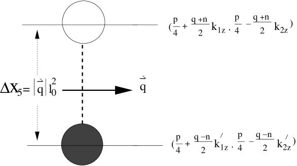
FIG. 2.: An illustration of the extremal dipole configuration. For a given center of mass momentum $q$, the dipole separation in the extra dimension is given by $ql_{0}^{2}$. $SO(4)$ quantum numbers of the particle and the hole are also indicated.

REFERENCES

• [1] R.Β B. Laughlin, Phys. Rev. Lett. 50, 1395 (1983).
• [2] S.-C. Zhang and J.-P. Hu, Science 294, 823 (2001).
• [3] C.Β N. Yang, J. Math. Phys. 19, 320 (1978).
• [4] C.Β N. Yang, J. Math. Phys. 19, 2622 (1978).
• [5] R. Jackiw and C. Rebbi, Phys. Rev. D 14, 517 (1976).
• [6] A. Belavin and A. Polyakov, Nucl. Phys. B 123, 429 (1977).
• [7] A. Belavin, A. Polyakov, A. Schwartz, and Y. Tyupkin, Phys. Lett. B 59, 85 (1975).
• [8] B.Β I. Halperin, Phys. Rev. B 25, 2185 (1982).
• [9] X.Β G. Wen, Phys. Rev. Lett. 64, 2206 (1990).
• [10] M. Stone, Phys. Rev. B 42, 8399 (1990).
• [11] K. Moon etΒ al., Phys. Rev. Lett. 71, 4381 (1993).
• [12] S. Weinberg and E. Witten, Phys. Lett. B 96, 59 (1980).
• [13] C. Kallin and B. Halperin, Phys. Rev. B 30, 5655 (1984).
• [14] V. Pasquier and F. Haldane, Nucl. Phys. B 516, (1998).
• [15] D. Lee, Phys. Rev. B 60, 5636 (1999).
• [16] A.Β R. Edmonds, Angular Momentum in Quantum Mechanics (Academic Press, 1957).
• [17] I. Affleck, T. Kennedy, E.Β H. Lieb, and H. Tasaki, Phys. Rev. Lett. 59, 799 (1987).
• [18] A. Connes, Noncommutative Geometry (Academic Press, 1994).
• [19] R. Szabo, hep-th/0109162 .
• [20] R. Laughlin and D. Pines, Proc. Natl. Acad. Sc. USA 97, 28 (2000).
• [21] G. Volovik, Phys. Rep. 351, 195 (2001).
• [22] G. Volovik, gr-qc/0112016 .
• [23] M.Β A. Vasiliev, hep-th/9910096 .
• [24] L. Susskind, hep-th/0101029 .
• [25] J. Talman, Special Functions, A Group Theoretic Approach (Benjamin Inc, Boston, MA, 1968).
• [26] M. Bander and C. Itzykson, Rev. Modern Phys. 38, 330 (1966).