Operating a phase-locked loop controlling a high-Q tuning fork sensor
for scanning force microscopy

Abstract

The implementation of a tuning fork sensor in a scanning force microscope operational at 300 mK is described and the harmonic oscillator model of the sensor is motivated. These sensors exhibit very high quality factors at low temperatures. The nested feedback comprising the sensor, a phase locked loop and a conventional $z$-feedback is analyzed in terms of linear control theory and the dominant noise source of the system is identified. It is shown that the nested feedback has a low pass response and that the optimum feedback parameters for the phase-locked loop and the $z$-feedback can be determined from the knowledge of the tuning fork resonance alone regardless of the tip shape. The advantages of this system compared to pure phase control are discussed.

I introduction

Since its invention by Binnig, Quate and Gerber [1], the scanning force microscope (SFM) has become a standard tool for the investigation of conducting and insulating surfaces on the atomic scale. Various imaging modes exist that can be classified to be either contact modes or dynamic modes [2]. The latter are characterized by the fact that the tip oscillates above the surface and the parameters of the oscillation are influenced by the tip-sample interaction. True atomic resolution has been achieved in this imaging mode [3]. Usually the cantilever oscillation is measured by optical means. Tuning fork sensors offer the possibility of non-optical detection of the cantilever oscillation via the piezoelectric effect [4, 5, 6]. It was demonstrated that atomic resolution is possible with these unconventional and very stiff sensors [7]. The fundamental limits to force detection with quartz tuning forks were disussed by Grober and co-workers in Ref. [8].

We employ the tuning fork sensors in a cryo-SFM setup in which the home-built microscope is operated in a ³He-cryostat at a temperature of 300 mK. Tuning fork sensors can be classified by the strength of the mixing between symmetric and antisymmetric mechanical oscillation modes. In the extreme case, one of the tuning fork prongs is firmly attached to a support [5] and extremely strong mode mixing occurs. In the first section of this paper we present evidence, that our sensors are in the weak mode mixing limit and that the simple harmonic oscillator model is therefore appropriate. In the second section we describe our nested SFM feedback system comprising the tuning fork sensor, a phase-locked loop and a conventional $z$-feedback. We present an analysis of the linear response and the noise of these feedbacks and show how the optimum settings for the feedback parameters can be found. These optimum parameters are found to be independent of the tip shape and the details of the tip sample interaction. The advantages of using a feedback with phase-locked loop for the very high $Q$ tuning fork sensors are discussed and a comparison is made with the phase control mode.

II Tuning fork sensors: a realistic model

In our dynamic mode SFM we employ the same type of tuning fork sensors previously discussed and calibrated in Refs. [6, 9]. Figure 1 shows a typical sensor. The commercially available tuning fork [10] is mounted on a print plate under an angle of about 10^∘. A 15 $\mu$m PtIr wire is glued [11] to the end face of one tuning fork prong and to a copper post which serves as the electrical contact to the tip. The free end of the wire is then etched electrochemically resulting in a sharp tip which will serve as a probe for the sample surface. The preparation technique impairs the symmetry of the tuning fork and we have to care about the effects on the oscillation properties.

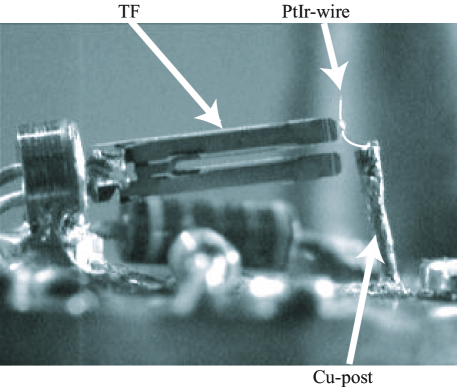
FIG. 1.: Tuning fork sensor used in our cryo-AFM.

Figure 2 shows the current through the tuning fork near resonance measured at a temperature of 4.2 K with an excitation voltage of $U_{0}=10$ $\mu$Vrms applied to the tuning fork contacts. The top graph is the magnitude of the current. The experimental details of the admittance measurements will be discussed later in the paper. In the following, we start with a mechanical model of the tuning fork sensor which eventually aims at the detailed understanding of such resonance curves. In particular, we will focus on the symmetry breaking effect of the tip prepraration.

We describe the mechanical oscillator with a coupled harmonic oscillator model driven by the voltage $U_{0}$ via the piezoelectric coupling constant $\alpha$.

$$m_{1}\ddot{x}_{1}+\gamma_{1}\dot{x}_{1}+k_{1}x_{1}+k_{c}x_{2}+\gamma_{c}\dot{x}_{2} = -\alpha U_{0}$$ (1)

$$m_{2}\ddot{x}_{2}+\gamma_{2}\dot{x}_{2}+k_{2}x_{2}+k_{c}x_{1}+\gamma_{c}\dot{x}_{1} = +\alpha U_{0}+F_{ts}(x_{2}).$$ (2)

The deflection of the two prongs is described by the coordinates $x_{i}$. The $m_{i}$ are the effective masses of the two prongs, the $k_{i}$ and $\gamma_{i}$ are their spring- and damping-constants, respectively. The tip is attached to prong 2 and interacts with the sample surface via the interaction force $F_{ts}(x_{2})$. Coupling between the prongs is described by coupling constants $k_{c}$ and $\gamma_{c}$.

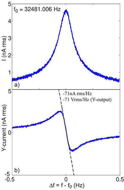
FIG. 2.: a) Current magnitude near the tuning fork resonance. b) Y-component of the current near resonance

The Eigenmodes of this oscillator (determined with $F_{ts}(x_{2})=0$) are given by

$\displaystyle\Omega_{1,2}^{2}=\omega_{0}^{2}\pm\omega_{c}^{2}\sqrt{1+\kappa^{2}}$

where $\omega_{0}^{2}=(k_{1}/m_{1}+k_{2}/m_{2})/2$, $\omega_{c}^{2}=k_{c}/\sqrt{m_{1}m_{2}}$ and $\kappa=(k_{1}/m_{1}-k_{2}/m_{2})/(2k_{c}/\sqrt{m_{1}m_{2}})$. In the case of $\kappa=0$, in particular when the two prongs are identical, the two Eigenmodes are the symmetric (the $x_{i}$ oscillate with zero phase difference) and the antisymmetric (the $x_{i}$ oscillate with a phase difference of $\pi$) mode. The metallic tuning fork contacts are arranged such that only the antisymmetric mode is excited by a driving voltage. For $\kappa\ll 1$ the two modes do not mix significantly and the symmetries of the modes are not strongly affected, while for $\kappa\gg 1$ each prong has its own resonance frequency where the other is hardly excited.

In the following we show that our tuning fork sensors are in the regime of negligible mode mixing, because the introduced asymmetry is small, i.e. $\kappa\ll 1$. We can rewrite the expression for $\kappa$ introducing $m_{1}=m$, $m_{2}=m+\Delta m$, $k_{1}=k$, $k_{2}=k+\Delta k$. Expanding up to first order in $\Delta m/m$, $\Delta k/k$ and $k_{c}/k$ we obtain

$\displaystyle\kappa=\frac{\Delta m/m-\Delta k/k}{2k_{c}/k}$

It can be seen that the additional mass on one prong can be compensated by increasing the spring constant, a fact exploited already in Ref. [12].

We estimate the additional spring constant $\Delta k$ of a thin wire attached to one prong. It is given by [13] $\Delta k=3\pi Er^{4}/(4L^{3})$, where $L$ denotes the length of the wire, $E$ is Young’s modulus of the material and $r$ is its radius. Typical wires have $r=7.5$ $\mu$m, $L=0.5$ mm, and $E=200-400$ GPa leading to $\Delta k=12-24$ N/m. With $k=14000$ N/m this results in $\Delta k/k\approx 10^{-3}$.

An estimate of the additional mass added to one arm of the tuning fork takes essentially the glue into account. The idealized drop of glue has the shape of a half-sphere with radius $r$ and volume $V=2\pi/3r^{3}$. Using the mass density of the H20E-epoxy $\rho=2600$ kg/m³ and a radius of 100 $\mu$m we obtain a mass of 5.44 $\mu$g. This weight has to be related to the mass of a single tuning fork arm which is 1.1 mg. This leads to the ratio $\Delta m/m=5\times 10^{-3}$.

The ratio $k_{c}/k$ can be estimated from finite element simulations of tuning fork sensors to be of the order of several percent [14].

From these estimates it seems to be reasonable that the employed sensors are in the limit of small mode mixing. An additional observation strongly supports this point of view: only very rarely is a second resonance observed in the admittance. Since the measured current detects only the antisymmetric component of the oscillation, strong mode mixing would make the second resonance visible.

Motivated by these estimates we approximate the equations of motions by $m_{1}=m_{2}=m$, $k_{1}=k_{2}=k$ and $\gamma_{1}=\gamma_{2}=\gamma$ and obtain

$$m\ddot{\xi}+(\gamma-\gamma_{c})\dot{\xi}+(k-k_{c})\xi = 2\alpha U+F_{ts}(s+\xi/2)$$ (3)

$$m\ddot{s}+(\gamma+\gamma_{c})\dot{s}+(k+k_{c})s = \frac{1}{2}F_{ts}(s+\xi/2)$$ (4)

with $s:=(x_{1}+x_{2})/2$ is the centre of mass coordinate and $\xi=x_{2}-x_{1}$ is the relative coordinate. The tip-sample interaction force couples the centre of mass motion to the relative motion. However, due to the extremely high stiffness of our tuning forks (of the order of $10^{4}$ N/m) a typical oscillation amplitude of 1 nm gives rise to a restoring force of $10^{-5}$ N. This is very large compared to typical tip-sample interaction forces of the order of 1 nN. Therefore we neglect the coupling and describe the tuning fork oscillation with the approximation $s=0$ which implies that $x_{1}=-x_{2}$ and $\xi=2x_{2}$. Inserting these relations into equation (3) leads to the single harmonic oscillator approximation for our tuning fork sensors, which we rewrite with $x=x_{2}$, $(k-k_{c})/m=\omega_{0}^{2}$ and $(\gamma-\gamma_{c})/m=\omega_{0}/Q$

$\displaystyle\ddot{x}+\frac{\omega_{0}}{Q}\dot{x}+\omega_{0}^{2}x=\frac{\alpha}{m}U+\frac{1}{m}F_{ts}(x).$

Summarizing the discussion of the tuning fork sensors, we have found two reasons why the single harmonic oscillator description is appropriate for our sensors: first, the added mass (the glue) is small compared to the mass of a single tuning fork arm. Second, the relative mechanical coupling strength of the two prongs is strong compared to the influence of the added mass and the added spring constant. In this respect these sensors are completely equivalent to other sensors with one prong firmly attached to the support which act essentially as an extremely stiff piezoelectric cantilever. In other respects there are important differences: we find quality factors $Q$ of up to 250000 under the UHV-conditions occuring in our evacuated sample space at a temperature of 300 mK. These values are 1-2 orders of magnitude larger than those reported for the other type of tuning fork sensors [5]. The implications of this will be discussed in the remainder of the paper.

III Admittance measurement

A Model for the admittance

The mechanical oscillation of tuning fork sensors is measured via the piezoelectric effect of the quartz crystal. The induced piezoelectric charge on one tuning fork electrode is given by $Q_{p}=\alpha\xi=2\alpha x$ and the corresponding piezoelectric current is $I_{p}=2\alpha\dot{x}$. In addition, a current of size $I_{c}=i\omega CU$ flows through the capacitance between the tuning fork contacts $C_{0}$ and the total current is therefore given by $I(\omega)=i\omega C_{0}U+2i\alpha\omega x(\omega)$. If we neglect the tip-sample interaction force we can determine $x(\omega)$ from the harmonic oscillator model and find

$\displaystyle I(\omega)=i\omega U\left(C_{0}+\frac{2\alpha^{2}/m}{\omega_{0}^{2}-\omega^{2}+i\omega\omega_{0}/Q}\right).$

Resonance curves like the one shown in Fig. 2a) can be excellently fitted with this equation.

Near resonance ($\omega\approx\omega_{0}$) the current is dominated by the piezoelectric contribution for our high $Q$ sensors and can be expanded to be

$$I(\omega)=\frac{2\alpha^{2}QU}{m\omega_{0}}\left(1-i\cdot\frac{2Q}{\omega_{0}}\cdot(\omega-\omega_{0})\right)+{\cal O}\left[(\omega-\omega_{0})^{2}\right].$$ (5)

The component of the current which is shifted by 90^∘ with respect to the driving voltage is depicted in Fig. 2b). It is proportional to the deviation of the excitation frequency from the resonance frequency. This fact is utilized for the AFM-feedback.

B Admittance measurement

We measure this current by using an I-U converter with a current to voltage conversion ratio of $K=10^{6}$ V/A at 32 kHz. A guard driver neutralizes the huge capacitance $C_{K}=1.8$ nF of the long coax-cable connecting the tuning fork in the cryostat and thereby increases the bandwidth of the I-U converter and reduces the output noise. It turns out that the output noise of the converter which was found in this setup to be $n_{IUC}=800$ nV/$\sqrt{\mbox{Hz}}$ at 32 kHz, dominates the noise in the whole AFM feedback.

Figure 3 shows the setup for the admittance measurement of the tuning fork. The fork (TF) is driven by voltage controlled oscillator (VCO) with typical excitation amplitudes between 10 $\mu$V and 1 mV depending on the $Q$-value of the tuning fork. The tuning fork current is converted into a voltage with the I-U converter (IUC). The resonance frequency of the tuning fork sensor depends on the tip sample interaction via the tip-sample separation $\Delta z$ and the tip-sample voltage $U_{ts}$ (see below).

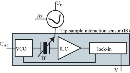
FIG. 3.: Setup for the measurement of the tuning fork admittance. It acts as the tip-sample interaction sensor (IS) in the SFM.

The resulting voltage is demodulated by the lock-in amplifier with sensitivity $S$ which determines the in-phase (X) and 90^∘ (Y) current components corresponding to the real and imaginary components in eq. (5). The output voltages up to first order in the frequency shift are given by

$$X_{res} = \frac{10\mbox{V}}{S}\cdot K\cdot\frac{\alpha^{2}QU}{\pi mf_{0}}$$

$$Y_{res} = -\frac{10\mbox{V}}{S}\cdot K\cdot\frac{\alpha^{2}Q^{2}U}{\pi^{2}mf_{0}^{2}}\cdot\Delta f=-X_{res}\cdot\frac{Q}{\pi f_{0}}\cdot\Delta f,$$

where we have introduced $f_{0}=\omega_{0}/(2\pi)$ and the frequency shift $\Delta f=f-f_{0}$. The $Y$-component of the signal is a linear indicator of the deviation from the resonance frequency which can be utilized for the AFM-feedback.

The spectral noise density on the output signals of the lock-in is given by $n_{Y}=10\mbox{V}/S\cdot n_{IUC}$. The integrated output noise $\delta Y_{res}$ depends on the lock-in time constant $\tau$ and on the order $n$ of its low-pass filter via

$\displaystyle\delta Y_{res}=c_{n}\times\frac{10\mbox{V}}{s}\times\sqrt{\frac{n_{IUC}^{2}}{2\pi\tau}}.$

The constants $c_{n}$ are calculated to be $c_{1}=1.25331$, $c_{2}=0.886227$, $c_{3}=0.767495$, $c_{4}=0.700624$, $c_{5}=0.655374$, $c_{6}=0.621742$. In our setup we use a lock-in time constant of $\tau=100$ $\mu$s corresponding to a bandwidth of 1.6 kHz and a fourth order low-pass filter. With $S=10$ mV this leads to $n_{Y}=800$ $\mu$V/$\sqrt{\mbox{Hz}}$ and to typical values of $\delta Y_{res}=22$ mV corresponding to a frequency noise of 0.3 mHz.

C Frequency shift and tip-sample interaction

The harmonic oscillator approximation for the tuning fork sensors allows us to apply the Hamilton-Yacoby perturbation result for the frequency shift [15]

$$\Delta f(\Delta z,U_{ts})=$$ (7)

$$-\frac{f_{0}}{2\pi Ak}\int_{0}^{2\pi}dx\;F_{ts}\left(\Delta z+A\sin x,U_{ts}\right)\sin x.$$

$$\approx \alpha\cdot\Delta U_{ts}+\beta\cdot\Delta z,$$ (8)

where $\alpha=\partial\Delta f(0,U_{0})/\partial U_{ts}$ and $\beta=\partial\Delta f(0,U_{ts})/\partial\Delta z$. The approximate expression of the frequency shift has been obtained by an expansion to first order in the tip-sample separation $\Delta z$ and the tip-sample voltage $U_{ts}$ which generates electrostatic tip-sample forces. The action of these quantities on the admittance measurement are indicated in Fig. 3.

IV Demodulation of the tuning fork sensor on resonance

A Step Response of the Sensor

For the AFM-operation it is crucial to determine the bandwidth of the tip-sample interaction sensor, i.e., the time it takes to respond to a given step in $\Delta z$ or $U_{ts}$. We first determine the step response of our sensor similar to Albrecht [2]. Following eq. (3) we assume that the oscillator is at all times driven by the force $2\alpha U_{0}\cos(\omega_{e}t+\Phi)$. For $t<0$ we excite on resonance, i.e. $\omega_{e}=\omega_{0}$ and assume that the oscillator performs its steady state oscillations. At $t=0$ we instantaneously change the resonance frequency of the oscillator to the new frequency $\Omega_{0}=\omega_{0}+\Delta\omega$ and seek solutions of eq. (3), neglecting $F_{ts}$, of the form

$\displaystyle\xi(t)=Y(t)\cos(\omega_{e}t+\Phi)+X(t)\sin(\omega_{e}t+\Phi)$

For $t<0$ the Amplitudes are $X(t)=A_{<}$ and $Y(t)=0$. For $t>0$ we find

$$Y(t) = A_{>}\cos\phi+Be^{-\omega_{0}t/(2Q)}\cos[\Delta\omega t+\theta-\Phi]$$ (9)

$$X(t) = -A_{>}\sin\phi-Be^{-\omega_{0}t/(2Q)}\sin[\Delta\omega t+\theta-\Phi]$$ (10)

The constants $B$ and $\theta-\Phi$, found from the boundary conditions at $t=0$, are given by

$$B^{2} = A_{>}^{2}+A_{<}^{2}+2A_{>}A_{<}\sin\phi$$ (11)

$$\cot(\theta-\Phi) = \frac{A_{>}\cos\phi}{A_{<}+A_{>}\sin\phi}$$ (12)

So far the results are generally valid and no approximations have been made. Now we consider approximate behaviour. For small frequency steps $\Delta\omega\ll\omega_{0}/(2Q)$ we find that

$\displaystyle Y(t)=2A_{<}\frac{Q\Delta\omega}{\omega_{0}}\left[1-e^{-\omega_{0}t/(2Q)}\cos\left(\Delta\omega t+\frac{2Q\Delta\omega}{\omega_{0}}\right)\right]$

Since the long-time behaviour of the response will be governed by the exponential decay we may approximate the response by

$\displaystyle Y(t)=2A_{<}\frac{Q\Delta\omega}{\omega_{0}}\left[1-e^{-\omega_{0}t/(2Q)}\right],$

i.e., a first order low-pass behaviour with bandwidth $f_{G}=f_{0}/(2Q)$. This gives immediately the step response of the demodulated current

$\displaystyle Y_{res}(t)=-X_{res}\cdot\frac{Q}{\pi f_{0}}\cdot\Delta f\cdot\left[1-e^{-\pi f_{0}t/Q}\right],$

or, after Fourier transformation

$\displaystyle Y_{res}(\omega)=k(\omega)\Delta f=-X_{res}\cdot\frac{Q}{\pi f_{0}}\cdot\Delta f\cdot\frac{1}{1+i\omega/(2\pi f_{G})}.$

B Measurement of the Sensor Response

A measurement of this low-pass behaviour is shown in Fig. 4. The measurement was performed at a temperature of 4.2 K with the tip at a distance of 80 nm from the surface of a GaAs/AlGaAs heterostructure in which a two-dimensional electron gas (2DEG) resides 34 nm below the surface. The tuning fork was driven on resonance with an AC-voltage of 10 $\mu$V applied to the tuning fork contacts. The 2DEG was employed as the metallic counter electrode of the tip. A DC tip-sample voltage of $U_{ts}=-9$ V was applied to the 2DEG while keeping the tip grounded. Following the idea of eq. (8) a low-frequency AC-voltage $\Delta U_{ts}=300$ mV was added in order to modulate the resonance frequency of the tuning fork. Fitting the low-pass behaviour (not shown) results in the characteristic frequency of the tuning fork $f_{G}=0.13$ Hz corresponding to $Q=116000$. In other experiments at low temperatures we achieved $Q$-values of up to 250000.

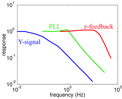
FIG. 4.: Various response functions of our feedback system. The curve labeled ‘Y-signal’ is the response function of the bare tuning fork sensor demodulated by the lock-in amplifier. The curve labelled ‘PLL’ is the response function of the phase-locked loop. The curve labeled ‘z-feedback’ is the response function of the $z$-feedback including the phase-locked loop.

In order to summarize the results of this section we want to emphasize the following points: the $Y$-output of the lock-in amplifier is used as the frequency detector in our setup. For small changes in resonance frequency $\Delta f\ll f_{G}=f_{0}/(2Q)$ the response shows low pass behaviour. Larger changes in resonance frequency lead to an oscillatory step response of the phase signal. High $Q$ sensors have a stronger tendency to an oscillatory response due the their higher $f_{G}$ as compared to lower $Q$ sensors.

V FM-detection with a phase-locked loop

FM detection was introduced in dynamic force microscopy by Albrecht and co-workers [2]. A theoretical description is due to Dürig and co-workers [16]. In such setups an FM demodulator is used for measuring the oscillation frequency of the cantilever. Phase-locked loops are one among many ways of FM demodulation. They are an established method of frequency measurement [17, 18]. The phase-locked loop was first employed in scanning probe measurements by Dürig and co-workers [19]. A digital version of a PLL has been developed by Ch. Loppacher and co-workers [20].

Due to the high $Q$-values of our sensors the response to changes in resonance frequency, in particular during the approach of the tip to the surface, is too slow to allow reasonable approach speeds. This is one reason why it is advantageous to employ a phase-locked loop in our setup. As we will show below, the phase-locked loop (PLL) increases the bandwidth of the response at the expense of increased noise.

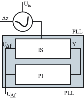
FIG. 5.: Phase-locked loop (PLL) comprising the interaction sensor (IS) and the P-I controller (PI).

A Linear response

The PLL-setup is schematically shown in Fig. 5. The output of the interaction sensor (IS), i.e., the phase signal $Y$, is fed into a P-I controller (PI). Its output $V_{\Delta f}$ is used as the input of the VCO in the interaction sensor. In the following we describe the PLL by the linear equations

$$Y(\omega) = k(\omega)(f_{res}(\omega)-f_{d}(\omega))$$ (13)

$$V_{\Delta f}(\omega) = R(\omega)Y(\omega)$$ (14)

$$f_{d}(\omega)-f_{0} = \eta V_{\Delta f}(\omega),$$ (15)

where $f_{res}$ is the resonance frequency of the tuning fork given by external parameters such as $\Delta z$ and $U_{ts}$, $f_{d}$ is the frequency output of the VCO driving the tuning fork and $f_{0}$ is the center frequency of the VCO around which $f_{d}$ can be modulated. The function $k(\omega)$ is the response of the interaction sensor shown in Fig. 3 including the lock-in demodulator with its frequency response defined by the lock-in time constant and filter characteristics, $R(\omega)$ is the response function of the P-I controller and $\eta$ is the response function of the VCO which is assumed to be frequency independent. The total response of the PLL depends crucially on the characteristic frequency of the P-I controller, $f_{PI}$, its gain $P$ and on the characteristic frequency of the tuning fork, $f_{G}$. Parameters are optimized, if

$$f_{PI}=f_{G}.$$ (16)

If $f_{PI}<f_{G}$ the response of the PLL is unnecessarily retarded while for $f_{PI}>f_{G}$ the response function develops an overshoot and tends to become unstable. If we regard $V_{\Delta f}$ as the output and $f_{res}$ as the input of the PLL we find the solution of the linear response equations

$\displaystyle V_{f}(\omega)=PLL(\omega)\cdot\left(f_{res}(\omega)-f_{0}\right)$

with the PLL-response function

$\displaystyle PLL(\omega)=\frac{1}{\eta}\cdot\frac{L(\omega)}{1+L(\omega)}$

and the open loop response defined as

$\displaystyle L(\omega):=R(\omega)k(\omega)\eta.$

The response becomes unstable at frequency $\omega_{0}$ if $\mbox{Arg}[L(\omega_{0})]=\pi$ and $\mbox{Abs}[L(\omega_{0})]>1$ (positive feedback). Stable feedback is therefore only achieved if $P$ is kept below a critical value $P_{c}$. In practice $P_{c}$ has to be determined experimentally.

At very low frequencies $R(\omega)$ is huge and $L(\omega)\gg 1$. In this limit $PLL(\omega)$ is constant with the value $1/\eta$. At frequencies much larger than $f_{PI}=f_{G}$ the function $R(\omega)$ is constant but $k(\omega)$ becomes very small such that $L(\omega)\ll 1$ and the response function decays like $k(\omega)$.

We now discuss the behaviour of this response function for the case that $f_{G}=f_{PI}$. In this case it reduces to

$\displaystyle PLL(\omega)=\frac{1}{\eta}\cdot\frac{1}{1+i\cdot\frac{f}{Pa\eta f_{G}}}=\frac{1}{\eta}\cdot\frac{1}{1+i\cdot\frac{f}{f_{PLL}}},$

where we have introduced $a=X_{res}Q/(\pi f_{0})$, i.e. to a low-pass behaviour with the new characteristic frequency

$\displaystyle f_{PLL}=Pa\eta f_{G}.$

The product $a\eta$ acts like an additional $P$-factor and the effective $P$-factor is $P_{eff}=Pa\eta$. The bandwidth of the PLL is a factor of $P_{eff}$ larger than the bandwidth of the interaction sensor itself. This is shown in Fig. 4 as the curve labeled ‘PLL’ which was measured with $\eta=0.1$ Hz/V, $a=71$ V/Hz and $P=2$. Higher bandwidths can be achieved with higher $P_{eff}$, however, the stability condition $P_{eff}<P_{c}$ and noise considerations constitute the upper experimental limits.

B Noise considerations

The dominating noise from the I-U converter can be represented as an equivalent noise source $n_{Y}(\omega)$ at the Y-output of the lockin. A linear response analysis starts from the equations

$$Y(\omega) = k(\omega)(f_{res}(\omega)-f_{d}(\omega))+n_{Y}(\omega)$$ (17)

$$V_{f}(\omega) = R(\omega)Y(\omega)$$ (18)

$$f_{d}(\omega)-f_{0} = \eta V_{f}(\omega).$$ (19)

The resulting noise term of the solution for $f_{G}=f_{PI}$ is

$$n_{PLL}(\omega)=P\cdot\frac{f-i\cdot f_{G}}{f-i\cdot f_{PLL}}\cdot n_{Y}(\omega).$$ (20)

At frequencies $f\gg f_{PLL},f_{G}$ the noise response is simply given by $P$, while for $f\ll f_{PLL},f_{G}$ the noise is given by the ratio $f_{G}/f_{PLL}=1/(Pa\eta)<1$. The low frequency noise is reduced by the PLL. However, since $f_{PLL}$ is small compared to the lockin bandwidth of about 530 Hz, the low frequency noise suppression is not relevant in practice for the integrated noise spectrum and to a good approximation the output noise of the PLL $\delta V_{\Delta f}$ is enhanced by the factor $P$ over the noise on the $Y$-output $\delta Y$:

$$\delta U_{\Delta f}=P\cdot\delta Y.$$ (21)

A measurement of the PLL-noise is shown in Fig. 6. Here, $\eta=0.1$ Hz/V, the tuning fork excitation was 10 $\mu$V. The lockin time constant $\tau=300$ $\mu$s at 24 dB/oct is responsible for the strong cut-off of the noise spectrum above 500 Hz. The I-U converter output noise $n_{IUC}$ was amplified by a factor 1000 by the lock-in and therefore has a value of 800 $\mu$V/$\sqrt{\mbox{Hz}}$. In the frequency range between 5 and 500 Hz the PLL-noise is enhanced by the factor $P=12$. At the lowest frequencies the noise is reduced in agreement with the above discussion. The integrated noise spectrum corresponds to an effective frequency noise of about 20 mHz/$\sqrt{\mbox{Hz}}$. If desired, parameters can be chosen such that the frequency noise is suppressed well below 1 mHz/$\sqrt{\mbox{Hz}}$ at the cost of bandwidth. For scanning we typically work with a PLL-noise of 10 mHz/$\sqrt{\mbox{Hz}}$.

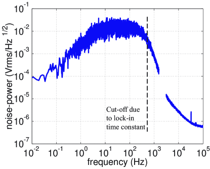
FIG. 6.: Output noise of the PLL in the full range of frequencies

VI The $z$-feedback

A Linear response

The PLL-feedback is part of the $z$-feedback loop as shown in Fig. 7. The PLL-output voltage $U_{\Delta f}$ is fed into the $z$-feedback P-I controller (PI) which drives the high-voltage amplifier (HV). This amplifier supplies the voltage for the $z$-piezo electrodes and thereby determines the tip-sample separation $\Delta z$. As a result of the force-distance interaction characteristic, $\Delta z$ and the tip-sample voltage $U_{ts}$ are translated into a resonance frequency of the interaction sensor [see eq. (8)] which is part of the PLL. For controlling the tip at constant height above the sample surface a certain $U_{set}$ is chosen corresponding to a certain frequency shift via $f_{set}=\eta U_{set}$. The feedback will then keep the tuning fork resonance frequency at $f_{set}$ by controlling $\Delta z$ during a scan.

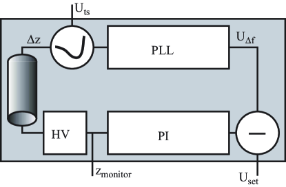
FIG. 7.: Scheme of the $z$-feedback consisting of the phase-locked loop (PLL), the P-I controller (PI), the high-voltage amplifier (HV) and the scan piezo tube.

In the following we discuss the $z$-feedback in a similar fashion to the PLL. Here the relevant linear equations are

$$\Delta f(\omega) = \alpha U_{ts}^{AC}(\omega)+\beta\Delta z(\omega)$$ (22)

$$\Delta z(\omega) = \mu\cdot\Delta U_{HV}(\omega)$$ (23)

$$U_{\Delta f}(\omega) = PLL(\omega)\cdot\Delta f(\omega)$$ (24)

$$e(\omega) = U_{set}-U_{\Delta f}(\omega)$$ (25)

$$\Delta U_{HV}(\omega) = PI(\omega)\cdot e(\omega)$$ (26)

Here $\mu$ is the (temperature-dependent) calibration of the $z$-piezo tube (e.g. 425 nm/70 V at 4.2 K), $U_{set}$ is the setpoint of the feedback, $PI(\omega)$ is the response of the $z$-feedback P-I controller and $e(\omega)$ is the error signal of the feedback loop. We are interested in the response of $\Delta z$ as a result of surface roughness on the sample. We can simulate this roughness by applying a sinusoidal AC tip-sample voltage $V_{ts}^{AC}$. The solution is

$\displaystyle\Delta z=Z(\omega)\cdot\frac{\alpha}{\beta}\cdot U_{ts}^{AC}.$

Here, the quantity $\alpha/\beta\cdot U_{ts}^{AC}$ plays the role of an effective surface roughness $\Delta z_{eff}$ and

$\displaystyle Z(\omega)=-\frac{M(\omega)}{1+M(\omega)}.$

with the open loop response

$\displaystyle M(\omega):=\beta\mu PI(\omega)PLL(\omega).$

In the limit of low frequencies $PLL(\omega)$ is constant, $PI(\omega)$ dominates and $\beta\mu PI(\omega)PLL(\omega)\gg 1$ such that $Z(\omega)$ is constant and given by $-z_{eff}$. In the limit of large frequencies this response decays like $PLL(\omega)$.

This feedback is stable, if $\mbox{Abs}[M(\omega)]<1$ at the frequency where $\mbox{Arg}[M(\omega)]=\pi$. This gives again an upper limit $P_{c}^{(z)}$ for possible $P_{z}$ values. $P_{c}^{(z)}$ depends on $\beta$ and therefore on the tip-sample interaction.

If we assume again that

$$f_{PLL}=f_{z}$$ (27)

the z-feedback response simplifies to

$\displaystyle Z(\omega)=-\frac{1}{1+i\cdot f/f_{FB}}$

with

$$f_{FB}=\frac{P_{z}\beta\mu}{\eta}\cdot f_{PLL}=P_{z}P\beta\mu a\cdot f_{G}.$$ (28)

Here the product $\beta\mu a$ acts as an additional $P$-factor and the effective value is $P_{eff}^{(z)}=P_{z}P\beta\mu a$ such that $f_{FB}=P_{eff}^{(z)}f_{G}$, i.e., the bandwidth of the $z$-feedback is again larger than the bandwidth of the PLL. This is demonstrated in Fig. 4 where the curve labeled ‘z-feedback’ was measured by varying the frequency of $U_{ts}^{AC}(\omega)$. The figure summarizes the resulting frequency characteristics of the two nested feedback-loops, i.e., the PLL and the $z$-feedback. It is demonstrated that the total system response is a low-pass, if all parameters are properly set. The bandwidth of the $z$-feedback can be increased by using higher $P_{eff}$, however, the stability criterion $P_{eff}<P_{c}^{(z)}$ and noise considerations constitute the experimental limits.

B Noise considerations

If we consider the contribution of the dominant I-U-converter noise in the $z$-feedback the relevant equations are

$$\Delta f(\omega) = \alpha U_{ts}^{AC}(\omega)+\beta\Delta z(\omega)$$ (29)

$$\Delta z(\omega) = \mu\cdot\Delta U_{HV}(\omega)$$ (30)

$$U_{\Delta f}(\omega) = PLL(\omega)\cdot\Delta f(\omega)+n_{PLL}(\omega)$$ (31)

$$e(\omega) = U_{set}-U_{\Delta f}(\omega)$$ (32)

$$\Delta U_{HV}(\omega) = PI(\omega)\cdot e(\omega)$$ (33)

The noise contribution $n_{PLL}(\omega)$ is the PLL output noise calculated earlier (see eq. (20)) which is dominated by the ouput noise of the I-U converter. The response to the PLL-output noise determined from these equations under the condition $f_{PLL}=f_{z}$ is

$\displaystyle n_{z}(\omega)=-\mu P_{z}\cdot P\cdot\frac{f-if_{G}}{f-if_{0}}\cdot n_{Y}(\omega).$

It is interesting to note that the bandwidth of the PLL does not enter the noise figure of the $z$-feedback. The integrated noise of the $z$-feedback is given by

$$\delta z=\mu P_{z}P\cdot\delta Y$$ (34)

Higher bandwidth of the $z$-feedback will lead to larger $z$-noise and for high quality imaging it is important to keep $\delta z$ as low as possible (typically of the order of 1 Å). On the other hand, reasonable scan speeds require high bandwidths of the order of several hundred Hz. This naturally leads to the question, how the optimum feedback parameters can be found from the above analysis for a given setup.

VII Optimum feedback parameters

The optimum feedback parameters are given by the following conditions:

1. The characteristic frequency of the PLL-PI-controller is identical to the characteristic frequency $f_{G}$ of the (tuning fork) sensor.

2. The characteristic frequency of the $z$-feedback P-I controller is identical to the PLL-bandwidth.

3. The $P_{eff}$ parameter of the PLL is well below the critical value $P_{c}$ where the PLL-feedback becomes unstable.

4. The $P_{eff}^{(z)}$ parameter of the z-feedback is well below the critical value $P_{c}^{(z)}$ where the z-feedback becomes unstable.

5. The $P_{eff}$ parameter of the PLL is small enough to give acceptable frequency noise.

6. The $P_{eff}^{(z)}$ parameter of the $z$-feedback is small enough to give acceptable $z$-noise.

We repeat the corresponding equations (16), (27), (21) and (34) below:

$$f_{PI} = f_{G}=\frac{f_{0}}{2Q}$$ (35)

$$f_{z} = f_{PLL}=P\eta\frac{X_{res}}{2\pi}$$ (36)

$$\delta U_{\Delta f} = P\cdot\delta Y$$ (37)

$$\delta z = \mu P_{z}P\cdot\delta Y$$ (38)

From these equations the optimum feedback parameters can be found as follows: First, the tuning fork resonance curve is measured and $f_{G}$ is determined from its half width at the $\sqrt{2}$-maximum value. This frequency determines the characteristic frequency to be set on the P-I controller of the PLL via eq. (35). The gain $P$ of this P-I controller is set such that the output noise of the PLL [$\delta U_{\Delta f}$, eq. (37)] corresponds to a reasonable frequency noise (typically 10 mHz for scanning in our setup). Next, the P-I parameters of the $z$-feedback are set such that eq. (36) is fulfilled. Finally, the gain $P_{z}$ of the $z$-feedback is adjusted according to the tolerable $z$-noise with the help of eq. (38). We typically keep the $z$-noise around 1 Å for normal scanning operation.

We emphasize that the optimum feedback parameters determined in this way do not depend on the tip shape or any details of the tip-sample interaction. Knowledge of the resonance curve of the sensor alone is sufficient for the optimum settings of the feedback.

For a given $z$-noise there is a certain freedom concerning the choice of the parameters $P$ and $P_{z}$, since according to eqs. (37) and (38) only their product needs to be kept constant. This freedom allows us to choose the bandwidth of the PLL either relatively high or relatively low in the span between $f_{G}$ and $f_{FB}$. If the PLL-bandwidth is chosen to be high, e.g. close to $f_{FB}$, the PLL will be able to track the resonance frequency with the same bandwidth as the $z$-feedback and $U_{\Delta f}$ will be constant throughout a scan. However, if the PLL bandwidth is chosen to be low, e.g. closer to $f_{G}$, the PLL can not track the resonance frequency with the same bandwidth as the $z$-feedback and appreciable error signals arise whenever there is a step on the surface. This is demonstrated in Fig. 8. The two images in the top row are topographic images of a detail of a Hall bar structure with AFM-written oxide lines in the bottom right corner. The left (right) image was taken with small (large) PLL-bandwidth at fixed bandwidth of the $z$-feedback. The bottom row shows the corresponding frequency error signal. It can be seen that with a slow PLL, an additional image can be obtained in which the contours of edges appear very sharp. With a fast PLL this contrast disappears completely. This ‘differential’ image of the surface can be very useful since it eliminates sample tilt and amplifies edges of small height nicely.

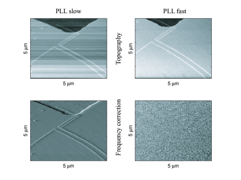
FIG. 8.: Left column: Topographic image (top) and frequency error signal (bottom) with small PLL bandwidth. Right column: the same with large PLL bandwidth.

VIII Effect of Q and k on the bandwidth

It becomes clear from the above discussion that the bandwidth of the $z$-feedback is given by eq. (28)

$\displaystyle f_{FB}=P_{z}P\beta\mu af_{G}=P_{z}P\beta\mu\frac{X_{res}}{2\pi}$

i.e., it is independent of the $Q$-factor of the tuning fork cantilever. This is not obvious, since high $Q$ cantilevers have a low $f_{G}$ and are therefore known to slow down the response. However, implemented in our nested feedback system the quality factor of the sensor is canceled from the final expression for the bandwidth. The only impact on the performance stems from the fact that the sensor response can only be described as a low-pass, if changes in frequency $\Delta f$ typically occurring during a scan are small compared to $f_{G}=f_{0}/(2Q)$.

The situation is different with the stiffness $k$ of the sensor which directly enters the quantity $\beta$, i.e., the slope of the $\Delta f(z)$ curve at the operating point. Softer sensors will lead to larger values of $\beta$ and thereby increase the bandwidth of the $z$-feedback.

Similar arguments play a role for the comparison of scanning in the attractive or repulsive part of the $\Delta f(z)$ curve. In the attractive part typical values of $\beta$ are much smaller than in the repulsive part. Therefore the bandwidth tends to be considerably larger for controlling in the repulsive regime.

IX Comparison to phase control

We briefly want to discuss why the use of the PLL is advantageous compared to phase control, where the phase change measured as the $Y$-output of the lock-in in our case is directly used for the $z$-controller without the intermediate PLL.

From a similar linear response analysis as performed in this paper for our nested system one finds that the same bandwidths of the $z$-feedback can be achieved with pure phase control. Enhancement of the bandwidth for scanning operation is therefore not the striking argument for the use of the additional PLL feedback.

However, there are several reasons, why we use the PLL:

1. The PLL increases the bandwidth of the tuning fork response when the $z$-feedback is not yet controlling, e.g. during the approach of the tip. The PLL allows the use of reasonable approach speeds.

2. The PLL increases the dynamic range of the frequency detection. The Y-signal of the lock-in depends linearly on the frequency shift only in a limited range of frequencies around resonance. With high $Q$ sensors this range can become so narrow (100 mHz) that during tip approach the frequency shift runs out of this range. The PLL avoids this problem by tracking the resonance. The frequency range that can be used with PLL is mainly determined by the VCO-settings. We typically use a range of 2 Hz.

3. The PLL allows to image with an additional adjustable frequency contrast (see Fig. 8).

4. When one measures $\Delta f(z)$-curves the PLL allows the clear distinction between conservative frequency shifts and dissipative effects [16, 21].

X Conclusion

In the first part of this paper we have shown that the tuning fork sensors that we use in our cryo-SFM setups can be well modeled by a single-harmonic oscillator despite the symmetry breaking wire that is attached to one tuning fork prong. In the second part of the paper we have analyzed the linear response of our nested feedback system comprising the interaction sensor, a phase-locked loop and a conventional $z$-feedback. We have demonstrated that the optimum feedback parameters of such a setup can be easily found and that they are independent of the tip shape and of the details of the tip-sample interaction. We have compared our setup to the conventional phase-control mode and discussed the advantages of the use of the phase-locked loop for high-Q cantilevers.

REFERENCES

- [1] G. Binnig, C.F. Quate, Ch. Gerber, Phys. Rev. Lett. 56, 930 (1986).
- [2] T.R. Albrecht, P. Grütter, D. Horne, D. Rugar, J. Appl. Phys. 69, 668 (1991).
- [3] F.J. Giessibl, Science 267, 68 (1995); S. Kitamura, M. Iwatsuki, Jpn. J. Appl. Phys. 34, L145 (1995); Y. Sugawara, M. Ohta, H. Ueyama, S. Morita, Science 270, 1648 (1995).
- [4] P. Günther, U. Ch. Fischer, K. Dransfeld, Appl. Phys. Lett. 48, 89 (1989); K. Karrai, R.D. Grober, Appl. Phys. Lett. 66, 1842 (1995); H. Edwards, L. Taylor, W. Duncan, A.J. Melmed, J. Appl. Phys. 82, 980 (1997); M. Todorovic, S. Schultz, J. Appl. Phys. 83, 6229 (1998).
- [5] F.J. Giessibl, Appl. Phys. Lett. 73, 3956 (1998).
- [6] J. Rychen, T. Ihn, P. Studerus, A. Herrmann, K. Ensslin, Rev. Sci. Instrum. 70, 2765 (1999).
- [7] F.J. Giessibl, Appl. Phys. Lett. 76, 1470 (2000).
- [8] R.D. Grober, J. Acimovic, J. Schuck, D. Hessman, P.J. Kindlemann, J. Hespanha, A.S. Morse, K. Karrai, I. Tiemann, S. Manus, Rev. Sci. Instrum. 71, 2776 (2000).
- [9] J. Rychen, T. Ihn, P. Studerus, A. Herrmann, K. Ensslin, Rev. Sci. Instrum. 71, 1695 (2000).
- [10] NTF3238 from SaRonix, 141 Jefferson Drive, Menlo Park, CA 94025, USA.
- [11] EPO-TEK H20E by Polyscience AG, Riedstrasse 13, CH-6330 Cham, Switzerland.
- [12] K.B. Shelimov, D.N. Davydov, M. Moskovits, Rev. Sci. Instrum. 71, 437 (2000).
- [13] D. Sarid, Scanning force microscopy, Oxford University Press, 1994.
- [14] T. Akiyama, private communication.
- [15] F.J. Giessibl, Phys. Rev. B 56, 16010 (1997).
- [16] U. Dürig, H.R. Steinauer, N. Blanc, J. Appl. Phys. 82, 3641 (1997).
- [17] U. Tietze, Ch. Schenk, Halbleiter Schaltungstechnik, Springer Verlag, Heidelberg, 1978 (Chapter 26).
- [18] R. Best, Phase-locked Loops: Theory, Design and Applications, McGraw-Hill, 1984; D.H. Wolaver, Phase-Locked Loop Circuit Design, Prentice Hall, 1991; F.M. Gardner, Phaselock Techniques, Wiley, 1979; A. Blanchard, Phase-Locked Loops: Appliccation to Coherent Receiver Design, Wiley, 1976.
- [19] U. Dürig, O. Züger, A. Stalder, J. Appl. Phys. 72, 1778 (1992).
- [20] Ch. Loppacher, M. Bammerlin, F. Battiston, M. Guggisberg, D. Müller, H.R. Hidber, R. Lüthi, E. Meyer, H.J. Güntherodt, Appl. Phys. A 66, S215 (1998); Ch. Loppacher, M. Bammerlin, M. Guggisberg, F. Battiston, R. Bennewitz, S. Rast, A. Baratoff, E. Meyer, H.-J. Güntherodt, Appl. Surf. Sci. 140, 287 (1999).
- [21] J. Rychen, T. Ihn, P. Studerus, A. Herrmann, K. Ensslin, H.J. Hug, P.J.A. van Schendel, H.J. Güntherodt, Appl. Surf. Sci. 157, 290 (2000).