Giant vortices in the Ginzburg-Landau description of superconductivity

Abstract

Recent experiments on mesoscopic samples and theoretical considerations lead us to analyze multiply charged ($n>1$) vortex solutions of the Ginzburg-Landau equations for arbitrary values of the Landau-Ginzburg parameter $\kappa$. For $n\gg 1$, they have a simple structure and a free energy ${\cal F}\sim n$. In order to relate this behaviour to the classic Abrikosov result ${\cal F}\sim n^{2}$ when $\kappa\rightarrow+\infty$, we consider the limit where both $n\gg 1$ and $\kappa\gg 1$, and obtain a scaling function of the variable $\kappa/n$ that describes the cross-over between these two behaviours of ${\cal F}$. It is then shown that a small-$n$ expansion can also be performed and the first two terms of this expansion are calculated. Finally, large and small $n$ expansions are given for recently computed phenomenological exponents characterizing the free energy growth with $\kappa$ of a giant vortex.

I Introduction

Recent experiments [1, 2, 3] have demonstrated that vortices of charge $n>1$, which are unstable in macroscopic type II superconductors [4], can exist in mesoscopic superconducting samples and can even be favored over configurations with multiple singly charged vortices. The Ginzburg-Landau description of superconductivity [5, 6, 7] appears to be an adequate framework to analyze these results. The magnetization response of a mesoscopic sample can be analytically understood by adding a surface energy contribution to the Ginzburg-Landau free energy of a giant-vortex in an infinite system [8, 9]. Moreover, full numerical solutions of the Ginzburg-Landau equations accurately reproduce the experimental findings [10, 11, 12].

Motivated by these experimental and theoretical results, we analyze in the present paper ‘giant’(i.e. $n>1$) vortex solutions of the Ginzburg-Landau equations. Well-known analytical results have been obtained in the London limit when the Ginzburg-Landau parameter $\kappa\to\infty$ [13, 7] and at the special dual-point value $\kappa=\frac{1}{\sqrt{2}}$ [7, 14]. Here, we take advantage of the supplementary parameter $n$, the vortex charge, and provide a simple analysis of the giant vortices for arbitrary values of $\kappa$. We begin in section 2, by recalling the Ginzburg-Landau equations and some elementary properties of their solutions. In section 3, we consider the large vorticity limit $n\gg 1$. The vortex structure takes the form of a circular normal core separated by a sharp boundary from the outside superconducting medium. As a consequence, the free energy $\cal{F}$ of a giant vortex is found to be proportional to its charge $n$ in contrast to the classic Abrikosov’s result ${\cal F}\sim n^{2}$ in the London limit. In order to relate the two results, we consider in section 4, the double limit in which both the vorticity $n$ and the Ginzburg-Landau parameter $\kappa$ are large and we obtain the scaling form ${\cal F}/2\pi\sim n\kappa\Phi(\kappa/n)$. The function $\Phi$ provides an explicit interpolation between Abrikosov’s result for $\kappa\gg n$ and the result of section 3 which is valid in the opposite limit $n\gg\kappa$. To complete our analysis of giant vortex solutions, we consider in section 5, the somewhat more formal $n\to 0$ limit, which has the advantage to be amenable to a simple and systematic expansion scheme; the free energy is obtained up to order $n^{2}$. In section 6, we compare our perturbative results (valid for arbitrary values of $\kappa$) to the known exact results at the dual point $\kappa=1/{\sqrt{2}}$. Besides checking consistency, we obtain a perturbative expansion of the free energy in the vicinity of the dual point and the large-$n$ expansion of phenomenological exponents introduced previously and computed numerically [9]. The large $n$ expansion proves to be fairly accurate for $n$ values as small as 3 or 4.

II The Ginzburg-Landau model of superconductivity

In the Ginzburg-Landau description of superconductivity [5, 6, 7] the two unknown fields are the complex order parameter $\psi=|\psi|e^{i\chi}$ and the potential vector ${\vec{A}}$ with ${\vec{\nabla}}\times{\vec{A}}={\vec{B}}$, where ${\vec{B}}$ is the local magnetic induction. These fields satisfy the following equations:

$$-({\vec{\nabla}}-i\frac{2\pi}{\phi_{0}}{\vec{A}})^{2}\psi = \frac{1}{\xi^{2}}\psi(1-|\psi{|^{2}}),$$ (1)

$${\vec{\nabla}}\times{\vec{\nabla}}\times{\vec{A}} = \frac{|\psi|^{2}}{\lambda^{2}}({\phi_{0}}\frac{{\vec{\nabla}}\chi}{2\pi}-{\vec{A}}).$$ (2)

Here, the flux quantum $\phi_{0}$ is given by $\phi_{0}={hc}/{2e},$ and the two characteristic lengths $\lambda$ (penetration depth or London length) and $\xi$ (coherence length) appear as phenomenological parameters. The Ginzburg-Landau parameter $\kappa$ is defined as their ratio, $\kappa=\frac{\lambda}{\xi}$. We shall measure lengths in units of $\lambda{\sqrt{2}}$, the magnetic field in units of $H_{c}/{\sqrt{2}\kappa}={\phi_{0}}/{4\pi\lambda^{2}}$ and the vector potential in units of ${\phi_{0}}/{2\sqrt{2}\pi\lambda}$. The Ginzburg-Landau free energy in units of ${H_{c}^{2}}{\xi^{2}}/{4\pi}$ is then given by:

$${\cal F}={\int}{1\over 2}B^{2}+{\kappa^{2}}(1-|\psi|^{2})^{2}+|({\vec{\nabla}}-i{\vec{A}})\psi{|^{2}}.$$ (3)

A giant vortex of vorticity $n$ is a solution of the Ginzburg-Landau equations with cylindrical symmetry $\psi(r,\theta)=f(r)\exp(in\theta),$ where $(r,\theta)$ are polar coordinates in the plane. The potential vector $\vec{A}$ can be chosen to lie in the plane and to have only a non-zero angular component $A_{\theta}(r)$. It is convenient to introduce an auxiliary function $g$ that represents the difference between the flux through a disk of radius $r$ and the total flux,

$$g(r)=rA_{\theta}(r)-n\,\,\,\,{\it i.e.}\,\,\,\,B=\frac{1}{r}\frac{dg}{dr}.$$ (4)

The free energy can be rewritten in terms of $f$ and $g$ as

$$\frac{1}{2\pi}{\cal F}=\int_{0}^{\infty}\left\{\left(\frac{df}{dr}\right)^{2}+\frac{f^{2}g^{2}}{r^{2}}+\kappa^{2}(1-f^{2})^{2}+\frac{1}{2r^{2}}\left(\frac{dg}{dr}\right)^{2}\right\}rdr.$$ (5)

The allied Ginzburg-Landau equations reduce to

$$\frac{d^{2}f}{dr^{2}}+\frac{1}{r}\frac{df}{dr}-\frac{1}{r^{2}}fg^{2} = -2\kappa^{2}f(1-f^{2}),$$ (6)

$$\frac{d^{2}g}{dr^{2}}-\frac{1}{r}\frac{dg}{dr} = 2f^{2}g.$$ (7)

It is useful to note that a very simple form of the free energy [7] is obtained by an efficient use of (6) and (7),

$$\frac{1}{2\pi}{\cal F}=2\kappa^{2}\int_{0}^{\infty}rdr(1-f^{2}).$$ (8)

A vortex of charge $n$ corresponds to functions $f$ and $g$ which satisfy $f(0)=0$ and $g(0)=-n$ at the origin and which obey $f(\infty)=1$ and $g(\infty)=0$ at infinity. Linearization of Eqs. (6, 7) around $f=1$ and $g=0$ shows that there exists two exponentially growing and two exponentially decaying spatial modes at $r=\infty$. In the same way, linearization for $r$ close to zero shows that there is one diverging mode with $f\sim r^{-n}$ and one neutral mode corresponding to changes in the vortex charge (note that at the level of Eqs. (6, 7), $n$ appears simply as a parameter and is not constrained to be an integer). Once one requires the diverging mode at $r=0$ to be absent and $g(0)=-n$, the expansion of $f$ and $g$ around $r=0$ depends on two arbitrary constants

$$f(r) = \left(\frac{r}{{\cal R}}\right)^{n}+{\cal O}(r^{n+1}),$$ (9)

$$g(r) = -n\left(1-\left(\frac{r}{r_{0}}\right)^{2}\right)+{\cal O}(r^{2n+2}).$$ (10)

The length scales $r_{0}$ and ${\cal R}$ are uniquely determined by the cancellation of the two divergent modes at $r=\infty$[15]; they cannot be calculated from a local analysis near 0. Their determination requires the behaviors around $r=0$ and $r=\infty$ to be connected. This can be done numerically for arbitrary parameter values or analytically when $n$ is either large or small as shown in the following sections.

One can note from the definition of $g$ (Eq. (4)) that $r_{0}$ is simply related to the value of the magnetic field at the position of the vortex:

$$B(0)=\left(\frac{1}{r}\frac{dg}{dr}\right)_{r=0}=\frac{2n}{r_{0}^{2}}.$$ (11)

III A giant vortex in the large vorticity limit

We first consider the structure of a giant vortex of charge $n$ for $n\gg 1$ and begin with simple estimates. It seems intuitively clear that the vortex core grows with its charge. So, for $n\gg 1$, one expects the vortex core to be much larger than the London penetration length. As a consequence, the magnetic induction should be approximately constant over the core. For a vortex of charge $n$ and core size $r_{c}$, one expects therefore $|B|=2n/r_{c}^{2}$ in the vortex core (the total flux divided by the core area with the chosen normalization) and $B=0$ outside. The magnetic energy of such a configuration is approximately $\int B^{2}/2\simeq 2\pi n^{2}/r_{c}^{2}$. Correlatively, one expects $\psi=0$ in the vortex core and $\psi=1$ outside and the corresponding energy contribution $\int\kappa^{2}(1-|\psi|^{2})^{2}\simeq 2\pi\kappa^{2}r_{c}^{2}$. The total Ginzburg-Landau energy (3) of such a configuration can therefore be estimated to be

$$\frac{1}{2\pi}{\cal F}\simeq\frac{n^{2}}{r_{c}^{2}}+\frac{\kappa^{2}}{2}r_{c}^{2}+\sigma(\kappa)r_{c},$$ (12)

where the last term on the right-hand side has been added to take into account the interfacial energy of the transition layer between the vortex core and the superconducting bulk. Minimizing Eq. (12) with respect to $r_{c}$ gives the dominant order estimates for the vortex size $r_{c}$ and for its free energy ${\cal F}$

$$r_{c}^{2} \sim \frac{\sqrt{2}n}{\kappa},$$ (13)

$$\frac{1}{2\pi}{\cal F} \simeq n\kappa\sqrt{2}+\left(\frac{\sqrt{2}n}{\kappa}\right)^{1/2}\sigma(\kappa)+{\cal O}(1).$$ (14)

The magnetic field inside the vortex core has the constant value

$$B=\sqrt{2}\kappa[1+\frac{\sigma(\kappa)}{2\kappa^{2}r_{c}}].$$ (15)

That is, in the vortex core $B$ is equal to $H_{c}$ plus a Gibbs-Thomson correction as expected at a curved normal/superconducting boundary (see e.g. [16, 17]). In the next subsections, we first present numerical solutions of the Ginzburg-Landau equations for various values of $n$ which confirm this simple picture of the giant vortex. This picture is then derived from a direct analysis of the Ginzburg-Landau equations in the large $n$ limit.

A Numerical results

Numerical solution of Eqs. (6,7) consists in solving a two-point boundary value problem (at $r=0$ and $r=\infty$) and can be achieved using several methods [18].

Shooting is generally easy to implement and robust when one mode needs to be cancelled at a boundary: a free parameter is adjusted (for example by dichotomy) at the other boundary until the required cancellation is obtained. In the present case, two diverging modes need to be cancelled at infinity which is more difficult to achieve. We kept a simple one parameter shooting by integrating from a large $r=r_{\infty}$ toward $r=0$. Of the two free parameters at $r_{\infty}$ one was used to cancel the diverging mode at $r=0$. The value of $g$ at $0$ was then given as a function of the other parameter (which could be adjusted to obtain a particular value of $n$ when desired).

We also implemented a relaxation method. The system of ordinary differential equations is replaced by a set of finite difference equations satisfied on a mesh of points, and the boundary conditions just appear as equations satisfied by the points located at the extremities of the mesh. A multi-dimensional version of Newton’s method provides a solution of these finite difference equations by an iterative procedure. This method requires the inversion of a matrix of size proportional to the number of points in the mesh. Because this matrix is block diagonal, it can be inverted in a very efficient manner. However, the efficiency of the relaxation method depends strongly on the starting point of the iteration: for example, it is useful to take the profile of a $n$-vortex as an initial guess for the $(n+1)$-vortex solution of the Ginzburg-Landau equations.

Numerical solutions for different values of $n$ are shown in Fig. 1. The plot of $f$ shows a well-defined interface between a normal region (where $f=0$) and a superconducting region $(f=1)$ (see Fig. 1a). The interface width does not increase with $n$ but remains of the order of $1/\kappa$. As expected, the interface has a well-defined limiting shape: in Fig. 1b, the curves represented in Fig. 1a are shifted in such a way that they take the value $1/2$ at the point $r=0$. The shifted curves superpose on one another almost perfectly. Only the curve for the small value $n=4$ shows a noticeable deviation from the limiting shape.

FIG. 1.: a) The function $f$ for $\kappa$ = 1.5 and n = 4,16,28,40,52. b) The different front profiles superposed on one another ($f=1/2$ is shifted to $r=0$).

The simple normal/superconducting interface picture for $n\gg 1$ is also confirmed by the graphs of $g$. In Fig. 2, $B(r)=1/r\ dg/dr$ is plotted for different values of $n$. The magnetic induction is close to $H_{c}=\sqrt{2}\kappa$ in the vortex interior and quickly decreases to zero in the interface region. Again, in the large $n$ limit, the curves can be put over one another by the same shifts as those used to superpose the different $f$’s in Fig. 1b.

FIG. 2.: The magnetic field for $\kappa^{2}=1.5$ and $n=4,16,28,40,52.$

B Asymptotic analysis of the Ginzburg-Landau equations for $n\gg 1$

It is instructive to see how the large-$n$ giant vortex structure arises in a direct analysis of the Ginzburg-Landau equations (6,7).

1 The vortex core

Since $g=-n$ at $r=0$ one expects $g$ to be of order $n$ in a whole region near $r=0$. Therefore, at dominant order in $n$, Eq. (6) for $f$ reduces to

$$\frac{d^{2}f}{dr^{2}}-\frac{1}{r^{2}}fg^{2}=0.$$ (16)

The solution of Eq. (16) can be obtained in a WKB manner but the important point is that $f$ is exponentially close to zero in the whole core region. Eq. (7) for $g$ thus simplifies to

$$\frac{d^{2}g}{dr^{2}}-\frac{1}{r}\frac{dg}{dr}=0.$$ (17)

At dominant order in $n$, $g$ is therefore given by

$$g(r)=-n\left(1-\left(\frac{r}{r_{0}}\right)^{2}\right).$$ (18)

Although Eq. (18) is identical to Eq. (10), it should be noted that it is not an expansion near zero but the full function $g$ in the vortex core at dominant order in $n$. Of course, Eq. (18) is nothing else but the constancy of $B$ in the vortex core.

Outside the vortex core the medium is in the superconducting phase, $f=1$ and $g=0$. In order to match these different solutions of Eqs.(6,7), we analyze the interface region (i.e. the boundary-layer in the usual matched asymptotics terminology).

It should be noted that $r_{c}$ the vortex core size and $r_{0}$ which is obtained from the second derivative of $g$ at the origin (Eq. (7)) coincide at leading order in $n$. Their difference is of the order of the planar normal/superconducting interface width and depends on the precise criterion used to measure the vortex core size (i.e. on the precise definition of $r_{c}$) as shown below.

2 Local equations near the interface

The solution (18) vanishes for $r=r_{0}$ and therefore the assumption $g\sim n$ under which it was derived breaks down at the interface. A different simplification of the Ginzburg-Landau equations can be made in the vicinity of $r_{0}$. We define a new variable $x$, centered around $r_{0}$, such that

$$r=x+r_{0}.$$ (19)

We assume (and will verify at the end) that $r_{0}\gg|x|$. Substituting (19) into (6,7) we obtain

$$\frac{d^{2}f}{dx^{2}}+\frac{1}{r_{0}}\frac{df}{dx}-\frac{g^{2}}{r_{0}^{2}}f = -2\kappa^{2}f(1-f^{2}),$$ (20)

$$\frac{d^{2}g}{dx^{2}}-\frac{1}{r_{0}}\frac{dg}{dx} = 2f^{2}g.$$ (21)

Comparing the magnitude of the different terms in these simplified equations, we obtain $f\sim 1,g\sim r_{0},x\sim 1$ and find that the first-order terms $df/dx$, $dg/dx$ on the l.h.s.  of (20,21) are subdominant. Introducing the rescaled functions $f_{0}=f$ and $G_{0}=g/r_{0}$, one derives at dominant order in $n$ (indicated by the subscript $0$) the ‘inner’ equations which describe the behaviour of the order parameter and the vector-potential in the interface region

$$\frac{d^{2}f_{0}}{dx^{2}} = -2\kappa^{2}f_{0}(1-f_{0}^{2})+G_{0}^{2}f_{0},$$ (22)

$$\frac{d^{2}G_{0}}{dx^{2}} = 2f_{0}^{2}G_{0}.$$ (23)

As expected, these equations are identical to the Ginzburg-Landau equations in one dimension (i.e. on an infinite line). Matching with the superconducting phase for $x\gg 1$ and the vortex core for $x\ll-1$ imposes the boundary conditions $f_{0}(+\infty)=1,G_{0}(+\infty)=0$ and $f_{0}(-\infty)=0$. This last condition implies, using (23), that $G_{0}$ behaves linearly when $x\to-\infty$

$$G_{0}\simeq ax+b.$$ (24)

In contrast to Eq. (6,7), the local system (22, 23) is invariant by translation. Once this is fixed (for example by imposing the arbitrary criterion $f_{0}(0)=1/2$) the functions $f_{0}$ and $G_{0}$ and the constant $b$ are uniquely determined (the value of $a$ is independent of this arbitrary choice). Finding $a$ and $b$ appears to require an explicit solution. This can be avoided, at least for $a,$ because the reduced system (22,23) retains the variational structure of the original equations and is invariant by translation in $x$. The locally conserved quantity $\cal E$ associated with this continuous symmetry reads (that is, the magnetic field in the vortex core)[5]

$${\cal E}=\frac{1}{2}\left(\frac{df_{0}}{dx}\right)^{2}+\frac{1}{4}\left(\frac{dG_{0}}{dx}\right)^{2}-\frac{1}{2}G_{0}^{2}f_{0}^{2}-\frac{\kappa^{2}}{2}(1-f_{0}^{2})^{2}.$$ (25)

Conservation of $\cal E$ between $-\infty$ and $+\infty$ leads to:

$$0={\cal E}(+\infty)={\cal E}(-\infty)=a^{2}/4-\kappa^{2}/2.$$ (26)

Thus, $a=\sqrt{2}\kappa$ and $B=H_{c}$ in the normal phase at dominant order in $n$, as expected.

3 Matching the vortex core and the interface region

In order to determine the constant $r_{0}$ and the interface position, we have to match the solutions in the vortex core and in the interface region.

Rewriting (10) in terms of the local variable $x$ leads to

$$g\simeq-n\left(1-(1+\frac{x}{r_{0}})^{2}\right)\simeq\frac{2n}{r_{0}}x\,\,\,\,\hbox{ hence }\,\,\,\,G_{0}=\frac{g}{r_{0}}\simeq\frac{2n}{r_{0}^{2}}x.$$ (27)

The family of solutions of (22,23) is $f_{0}(x-x_{c}),G_{0}(x-x_{c})$ with the asymptotic behavior

$$G_{0}(x-x_{c})=\sqrt{2}\kappa(x-x_{c})+b$$ (28)

Identifying the two local expressions (27) and (28) for the function $g$ in their common region of validity $r=r_{0}+x$ with $|x|\ll r_{0}$, and $x\to-\infty$ determines $r_{0}$ and $x_{c}$

$$r_{0}^{2} \simeq \sqrt{2}n/\kappa$$ (29)

$$x_{c} = \frac{b}{\sqrt{2}\kappa}$$ (30)

The large-$n$ asymptotic estimate of $r_{0}$ (which agrees with Eq. (13)) is compared with numerical results in Fig. 3 a.

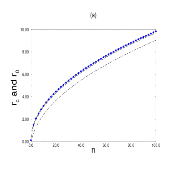
FIG. 3.: a) The vortex-core size $r_{c}$ (dot-dashed curve) and the length $r_{0}$ (solid line curve) are plotted for $\kappa=1.5$ and for values of $n$ ranging from 1 to 100. The dashed curve is the large-$n$ asymptotic estimate (13). The dots represent the next-to-leading order asymptotic expression (38), using the numerical value $\sigma(1.5)\simeq-1.172.$ b) Difference $\Delta_{r_{0}}$ between $r_{0}$ and its asymptotic expression (38).

4 Large $n$ limit of the energy

The free energy of a giant vortex can now be calculated for $n\gg 1$. Using (6) and integrating by parts, the free energy (5) becomes:

$$\frac{1}{2\pi}{\cal F}=\int_{0}^{\infty}rdr\left\{\frac{B^{2}}{2}+\kappa^{2}-\kappa^{2}f^{4}\right\}.$$ (31)

Completing the square with the first two terms inside the brackets and using relation (4) between $B$ and $g$, leads to

$$\frac{1}{2\pi}{\cal F}=n\kappa\sqrt{2}+\int_{0}^{\infty}rdr\left\{\frac{1}{2}\left(\frac{1}{r}\frac{dg}{dr}-\kappa\sqrt{2}\right)^{2}-\kappa^{2}f^{4}\right\}.$$ (32)

The function

$$S(r)=\frac{1}{2}\left(\frac{1}{r}\frac{dg}{dr}-\kappa\sqrt{2}\right)^{2}-\kappa^{2}f^{4},$$ (33)

is non-zero only in the vicinity of $r_{0}$. Hence, $S$ can be considered to be a function of $x=r-r_{0}$. Replacing the functions $f(r)$ and $g(r)$ in (33) by their dominant order approximations $f_{0}(x-x_{c})$ and $G_{0}(x-x_{c}),$ respectively, solutions of (22, 23), we obtain

$$\int_{0}^{\infty}rS(r)dr\simeq r_{0}\int_{-\infty}^{\infty}S(x)dx=r_{0}\int_{-\infty}^{\infty}\left\{\frac{1}{2}\left(\frac{dG_{0}}{dx}-\kappa\sqrt{2}\right)^{2}-\kappa^{2}f_{0}^{4}\right\}dx=r_{0}\sigma(\kappa).$$ (34)

The last integral is nothing else but the surface energy $\sigma(\kappa)$ of a one-dimensional domain wall between normal and superconducting phases [5, 19, 20] (see appendix A). Using (34) in (32) gives exactly the large $n$ expression (14) of the free energy of a $n$ giant-vortex with $\sigma(\kappa)$ the surface energy of a one dimensional normal/superconducting interface. The expression (14) is valid for any value of $\kappa$ in the limit $n\to\infty$. It is compared to the numerical results (for $\kappa=1.5$ ) in Fig. 4.

FIG. 4.: Free energy $\frac{\cal F}{2\pi n}$ as a function of $n$ for $\kappa$ = 1.5 (solid line). The horizontal dot-dashed line is the asymptotic value $\kappa\sqrt{2}\simeq 2.121$. The dashed curve is the large $n$ behaviour (14), using the numerical value $\sigma(1.5)\simeq-1.172.$

5 Finite-$n$ correction to $H_{c}$

The leading finite-$n$ correction to $B$ in the vortex core can be derived from the previous results. Integrating (8) by parts leads to

$$\frac{1}{2\pi}{\cal F}=\kappa^{2}\int_{0}^{\infty}r^{2}\phi(r)dr\,\,\,\hbox{ with }\,\,\,\phi(r)=2f(r)\frac{df}{dr}.$$ (35)

The function $\phi(r)$ is localized at the position of the front and its width is of the order $1/\kappa$. Using the local variable $x=r-r_{0}$ defined in (19), the equation (35) can be rewritten, in the large $n$ limit, as:

$$\frac{1}{2\pi}{\cal F}=\kappa^{2}r_{0}^{2}+2\kappa^{2}r_{0}\int_{-\infty}^{\infty}x\phi(x)dx+{\cal O}(1).$$ (36)

The integral in Eq. (36) can be expressed in terms of the interface energy (see appendix A):

$$2\kappa^{2}\int_{-\infty}^{\infty}\phi(x)xdx=2\kappa^{2}\int_{-\infty}^{\infty}\left((1-f_{0}^{2})-\frac{1}{\kappa\sqrt{2}}\frac{dG_{0}}{dx}\right)dx=\frac{3}{2}\sigma(\kappa).$$ (37)

Comparing (36) with (14) provides the large $n$ expansion of $r_{0}$ up to the second order

$$r_{0}=\left(\frac{\sqrt{2}n}{\kappa}\right)^{1/2}-\frac{\sigma(\kappa)}{4\kappa^{2}}+{\cal O}\left(\frac{1}{n^{1/2}}\right).$$ (38)

The vortex size $r_{c}$, defined by the criterion $f(r_{c})=1/2$, can be meaningfully calculated to the same order:

$$r_{c}=r_{0}+x_{c}$$ (39)

with $x_{c}$ given by Eq. (30).

In order to verify numerically these relations, we first computed the value of the magnetic field at the origin using the following relation, that derives from (4) and (7):

$$B(0)=-2\int_{0}^{\infty}\frac{f^{2}g}{r}dr.$$

This allowed us to obtain $r_{0}$, from (11), with a good precision. The vortex size $r_{c}$ was found from the equation $f(r_{c})=1/2$. In Fig. 3a, the two numerical curves for $r_{0}$ and $r_{c}$ are plotted as a function of $n$. To the leading order in $n$, these two curves differ by a constant $x_{c}\simeq-0.797\ldots$, function of $\kappa$ only, as predicted by Eq. (39). Solving independently the ‘inner’ Ginzburg-Landau equations (22,23), we found that the unique value of $b$ such that $f_{0}(0)=1/2$ is given by $b\simeq 1.691\ldots$ Hence the relation (30) between $x_{c}$ and $b$ is verified. We also tested the accuracy of the large $n$ asymptotic expansion of $r_{0}$ to the first order (13) and to the second order (38). The difference between $r_{0}$ and Eq. (38), hardly visible in Fig. 3a, is plotted in Fig. 3b. The agreement is very good.

Substituting this value of $r_{0}$ in (11), we obtain the field value inside the core

$$B(0)=\kappa\sqrt{2}+\frac{\sigma(\kappa)}{2^{3/4}\sqrt{\kappa n}}+{\cal O}\left(\frac{1}{n}\right).$$ (40)

Hence, when $n\to\infty$, the field at the origin is indeed the thermodynamic critical field $H_{c}=\kappa\sqrt{2}$ with a Gibbs-Thomson correction as expected (15).

IV Relation to Abrikosov’s formula

The self-energy of a unit vortex was first calculated by Abrikosov [13, 7] in the large $\kappa$ limit

$$\frac{1}{2\pi}{\cal F}=\log\kappa+0.081.$$ (41)

In the previous section we have studied the case $n\to\infty$ keeping $\kappa$ fixed and finite. In order to relate our results to the classical calculation of Abrikosov, we consider in this section the double limit $n\to\infty$ and $\kappa\to\infty$ keeping the ratio $u=\kappa/n$ finite and fixed. With these assumptions, we shall see that the Ginzburg-Landau equations decouple and that a scaling form is obtained for the free energy

$$\frac{1}{2\pi}{\cal F}=n\kappa\Phi(\kappa/n).$$ (42)

The function $\Phi$ is plotted in Fig. 5.

FIG. 5.: The scaling function $\Phi$ as a function of the variable $u$ (solid line). The dot-dashed curve and the dashed curve represent, respectively, the large $u$ (67) and small $u$ (78) approximations.

A The double limit $n\gg 1$ and $\kappa\gg 1$

After rescaling the function $g$ by a factor $1/n$, and introducing the ratio $u=\kappa/n$, the Ginzburg-Landau equations become:

$$\frac{1}{n^{2}}\left(\frac{d^{2}f}{dr^{2}}+\frac{1}{r}\frac{df}{dr}\right) = -2u^{2}f(1-\frac{1}{2u^{2}r^{2}}g^{2}-f^{2}),$$ (43)

$$\frac{d^{2}g}{dr^{2}}-\frac{1}{r}\frac{dg}{dr} = 2f^{2}g;$$ (44)

the boundary conditions are $f(0)=0$ and $g(0)=-1$ at the origin, and $f(\infty)=1$ and $g(\infty)=0$ at infinity. In the $n\to\infty$ limit, there are two domains where $f$ is slowly varying and the derivative terms in Eq. (43) can be neglected

$$f = 0\,\,\,\hbox{ for }\,\,\,r\leq R,$$ (45)

$$f = \left(1-\frac{g^{2}}{2u^{2}r^{2}}\right)^{1/2}\,\,\,\hbox{ for }\,\,\,r\geq R.$$ (46)

As shown below, these two domains match through a boundary layer at $r=R$ where $f$ has a rapid variation but remains small. Matching the two slowly varying expressions (46) of $f$ requires that $f(R)=0$ in the second one and gives

$$g(R)=-\sqrt{2}uR.$$ (47)

Substituting (46) in (44) leads to the following closed equations for $g$:

$$\hbox{ for }\,\,\,r\leq R\,\,\,\,\,\,\,\,\frac{d^{2}g}{dr^{2}}-\frac{1}{r}\frac{dg}{dr} = 0,$$ (48)

$$\hbox{ for }\,\,\,r\geq R\,\,\,\,\,\,\,\,\frac{d^{2}g}{dr^{2}}-\frac{1}{r}\frac{dg}{dr} = 2g\left(1-\frac{g^{2}}{2u^{2}r^{2}}\right).$$ (49)

From (48), one has

$$\hbox{ for }\,\,\,r\leq R\,\,\,\,\,\,\,\,g(r)=-1+\left(\frac{r}{r_{0}}\right)^{2}.$$ (50)

Continuity of the function $g$ and of its derivative at $R$, and equation (47) imply that

$$g(R)=-1+\left(\frac{R}{r_{0}}\right)^{2}=-\sqrt{2}uR,$$ (51)

$$g^{\prime}(R)=2\frac{R}{r_{0}^{2}}=\frac{2}{R}-2\sqrt{2}u,$$ (52)

(the second equality of (52) is derived using (51)). The scaling limit for the free energy when $n\to\infty$ and $\kappa\to\infty$ is obtained from (8) and (46)

$$\frac{1}{2\pi}{\cal F}=n\kappa\left(uR^{2}+\frac{1}{u}\int_{R}^{\infty}\frac{g^{2}}{r}dr\right)=n\kappa u\left(R^{2}+2\int_{R}^{\infty}rh^{2}(r)\right),$$ (53)

where we have introduced a function $h$ :

$$g\equiv h{\sqrt{2}ur}.$$ (54)

This provides the explicit expression of the interpolating function $\Phi$ (42)

$$\Phi(u)=u\left(R^{2}+2\int_{R}^{\infty}rh^{2}(r)\right).$$ (55)

In order to calculate explicitly $\Phi$ one has to determine the position $R$ of the front and the function $h$ as a function of $u=\kappa/n$. In terms of $h$, Eq. (49) becomes

$$\frac{d^{2}h}{dr^{2}}+\frac{1}{r}\frac{dh}{dr}-\frac{1}{r^{2}}h=2h(1-h^{2}),$$ (56)

and, from (47), the boundary conditions for $h$ are

$$h(R)=-1\,\,\,\,\,\hbox{ and }\,\,\,\,\,h(\infty)=0.$$ (57)

Relation (52) implies, however, one more condition on $h$:

$$h^{\prime}(R)=\frac{\sqrt{2}}{uR^{2}}-\frac{1}{R}\,\,.$$ (58)

The differential equation (56) with the two boundary conditions (57) and the supplementary condition (58) is overdetermined: there is a unique value of $R$ such that all the conditions can be satisfied. Indeed, equation (56) with the boundary conditions (57) has a unique solution for any given value of $R$, i.e. for a given $R$, the value of $h^{\prime}(R)$ is unique and can easily be computed numerically by solving (56) by a shooting method; once $h^{\prime}(R)$ is known, $u$ is determined as a function of $R$ from (58)

$$\frac{u}{\sqrt{2}}=\frac{1}{R+R^{2}h^{\prime}(R)}.$$ (59)

Inverting this relation gives $R$ as a function of $u$ (Fig. 6) and the function $\Phi$ using (55). This calculation can be performed analytically when $u$ is either very large or very small as shown below.

Before considering these limits, we complete the above analysis by giving the boundary-layer equation satisfied by $f$ in the neighbourhood of $r=R$. It is convenient to introduce the local variable $x=r-R$. Assuming that $f$ remains small in the neighbourhood of $r=R$ and keeping the dominant contribution of each term of Eq. (43), we obtain

$$\frac{1}{n^{2}}\left(\frac{d^{2}f}{dx^{2}}+\frac{1}{R}\frac{df}{dx}\right)=2u^{2}f(-2h^{\prime}(R)x+f^{2}).$$ (60)

A consistent dominant balance between the different terms of Eq. (60) is obtained when $f/(x^{2}n^{2})\sim fx\sim f^{3}$. Therefore, as assumed, $f$ evolves on a short scale $x\sim n^{-2/3}$ around $r=R$ but remains small $f\sim n^{-1/3}$. With the rescaled coordinate and function, $\xi=x(4u^{2}h^{\prime}(R))^{1/3}n^{2/3},F=(nu)^{1/3}(\sqrt{2}h^{\prime}(R))^{-1/3}f$, the boundary-layer equation reads

$$\frac{d^{2}F}{d\xi^{2}}=-\xi F+F^{3}.$$ (61)

The two different functions of Eq. (46) can be matched through the solution of (the Painlevé) Eq.  (61).

FIG. 6.: The inverse of $R$ plotted as a function of the scaling variable $u$ (solid line). The dashed curve represents the linear behaviour of $1/R$ for large values of $u$ (65), and the dotted curve shows the asymptotic behaviour for small values of $u$ (73).

B The large $u$ limit $(\kappa\gg n\gg 1)$

Recalling that $R$ and $r_{0}$ are positive, we see from (52) that $R\leq{1}/({\sqrt{2}u}).$ Therefore, when $u$ tends to infinity, $R$ tends to 0. In the large $u$ limit, equations (48) and (49) reduce to:

$$\frac{d^{2}g}{dr^{2}}-\frac{1}{r}\frac{dg}{dr}=2g,$$ (62)

with the boundary conditions $g(0)=-1$ and $g\to 0$ at infinity. The solution of this equation is readily obtained:

$$g(r)=-r\sqrt{2}K_{1}(r\sqrt{2})\,\,\,\,\hbox{ and therefore }\,\,\,\,h(r)=-K_{1}(r\sqrt{2})/u.$$ (63)

where $K_{1}$ is the modified Bessel function of order 1. Using the behaviour of $K_{1}$ in the vicinity of zero (see Appendix B), we deduce that

$$h^{\prime}(R)\simeq\frac{1}{\sqrt{2}uR^{2}}.$$ (64)

Substituting (64) in (59) leads to

$$R\simeq\frac{1}{\sqrt{2}u}.$$ (65)

Inserting (63) and (65) in the the expression (53) for the free energy, we obtain

$$\frac{1}{2\pi}{\cal F} \simeq \frac{n\kappa}{u}\left[\frac{1}{2}+\int_{1/u}^{\infty}r(K_{1}(r))^{2}dr\right]=\frac{n\kappa}{2u}\left\{1+\frac{1}{u^{2}}\left[K_{0}\left({1\over u}\right)K_{2}\left({1\over u}\right)-K_{1}\left({1\over u}\right)^{2}\right]\right\},$$ (66)

$$\simeq \frac{n\kappa}{u}(\ln u+\ln 2-\gamma)\simeq n^{2}\left(\ln\left(\frac{\kappa}{n}\right)+0.116\right),$$ (67)

where the $K_{\nu}$ are modified Bessel functions and $\gamma$ is the Euler constant [21]. This relation generalizes the classical result (41) of Abrikosov to the case of a giant vortex. Indeed, the structure of the giant vortex is very similar to the $n=1$ case with $f$ varying on a fast scale of order $n/\kappa$ and $g$ on a slow scale of order one. However, the structure of $f$ is simpler in the large $n$ limit (being $0$ for $r$ less than $n/(\sqrt{2}\kappa)$ and linked to $g$ otherwise) than for general $n$. This is the reason why no new constant needs to be numerically determined in (67).

C The small $u$ limit $(n\gg\kappa\gg 1)$

In the small $u$ case, the length $R$ tends to infinity. Defining a local variable $x=r-R$, the differential equation (56) for $h$ becomes

$$\frac{d^{2}h}{dx^{2}}+\frac{1}{R+x}\frac{dh}{dx}-\frac{1}{(R+x)^{2}}h=2h(1-h^{2}),$$ (68)

with the following boundary conditions

$$h(x=0)=-1\,\,\,\,\,\hbox{ and }\,\,\,\,\,h(\infty)=0.$$ (69)

When $R\to\infty$, the equation (68) reduces to:

$$\frac{d^{2}h}{dx^{2}}=2h(1-h^{2}).$$ (70)

The solution that satisfies the boundary conditions is:

$$h(x)=-\sqrt{2}\left(1-\tanh^{2}(\sqrt{2}(x+x_{0}))\right)^{1/2}\,\,\,\,\,\hbox{ with }\,\,\,\,\,\tanh(\sqrt{2}x_{0})=\frac{1}{\sqrt{2}}.$$ (71)

¿From this expression, we derive that

$$h^{\prime}(r=R)=h^{\prime}(x=0)=1.$$ (72)

Substituting this result in (59) leads to the small $u$ behaviour of $R$

$$R\simeq\left(\frac{\sqrt{2}}{u}\right)^{1/2}.$$ (73)

The subleading behaviour of $R$ as a function of $u$ is found by retaining only the first order term in $1/R$ in (68):

$$\frac{d^{2}h}{dx^{2}}+\frac{1}{R}\frac{dh}{dx}=2h(1-h^{2}),$$ (74)

with the same boundary conditions as in (69). This equation can be solved perturbatively, but we only need to determine the correction to equation (72); i.e. we need to calculate the coefficient $C$ such that $h^{\prime}(r=R)=1+C/R$. We use an argument of energy conservation. Defining

$${\cal E}_{2}=\frac{1}{2}\left(\frac{dh}{dx}\right)^{2}-h^{2}+\frac{h^{4}}{2},$$

we readily obtain from (74) that

$$\frac{d{\cal E}_{2}}{dx}=-\frac{1}{R}\left(\frac{dh}{dx}\right)^{2}.$$

Integrating this relation from $0$ to $\infty$ and evaluating the energy ${\cal E}_{2}$ at both ends leads to

$$C=\int_{0}^{\infty}\left(\frac{dh}{dx}\right)^{2}dx.$$ (75)

Using the 0th-order solution (71) for $h$ in (75) we obtain

$$h^{\prime}(r=R)=h^{\prime}(x=0)=1+\left(\frac{2\sqrt{2}-1}{3}\right)\frac{1}{R}.$$ (76)

Substituting this result in (59) and solving for $R$ leads to

$$R\simeq\left(\frac{\sqrt{2}}{u}\right)^{1/2}\left(1-2^{-1/4}\frac{\sqrt{2}+1}{3}u^{1/2}+{\cal O}(u)\right).$$ (77)

Substituting the expressions (77) and (71) for $R$ and $h,$ respectively, in (53) we obtain the free energy

$$\frac{1}{2\pi}{\cal F}\simeq n\kappa\left(uR^{2}+2R\int_{0}^{\infty}h^{2}(x)dx\right)\simeq n\kappa\sqrt{2}\left(1-\frac{4}{3}(\sqrt{2}-1)2^{1/4}\left(\frac{\kappa}{n}\right)^{1/2}+{\cal O}(u)\right).$$ (78)

These results are consistent with those obtained in section 3. In fact the small $u$ limit amounts to first taking the limit $n\to\infty$ and then taking $\kappa\to\infty$. For instance, it can be shown that equation (38) reduces to (77) in the $\kappa\to\infty$ limit. Moreover, comparing (78) with (14) we retrieve the asymptotic behaviour of the surface tension in the large $\kappa$ limit [7, 20]:

$$\sigma(\kappa)\simeq-\frac{4\sqrt{2}}{3}(\sqrt{2}-1)\kappa^{2}\simeq-0.7810\kappa^{2}.$$ (79)

V A vortex in the small vorticity limit

The winding number $n$ must be a priori an integer because the phase of the wave function $\psi$ has to be a $2\pi$ periodic function. However, as already noted, in the cylindrically symmetric Ginzburg-Landau equations (6,7), $n$ appears only as a parameter in the boundary condition at the origin and can be given any real value. In this section, we take $n$ to be close to 0 and determine perturbatively the solutions of (6,7) and the free energy.

Away from the origin $r=0$, $f$ is close to one and $g$ is small. Thus, we expand $f$ and $g$ as follows,

$$f=1+nf_{1}+n^{2}f_{2}+\ldots\,\,\,\hbox{ and }\,\,\,g=ng_{1}+n^{2}g_{2}+\ldots$$ (80)

The functions $f_{1}$,$g_{1}$, $f_{2}$, $g_{2}$… satisfy a hierarchical system of linear differential equations that can be solved recursively by imposing the boundary conditions: $f_{i}\to 0$ and $g_{i}\to 0\,\,\,$ when $r\to\infty$, for all $i\geq 1.$

Thus the first order terms $f_{1}$ and $g_{1}$ are solutions of

$$\frac{d^{2}f_{1}}{dr^{2}}+\frac{1}{r}\frac{df_{1}}{dr} = 4\kappa^{2}f_{1},$$ (81)

$$\frac{d^{2}g_{1}}{dr^{2}}-\frac{1}{r}\frac{dg_{1}}{dr} = 2g_{1}.$$ (82)

Implementing the boundary and the matching conditions, we obtain

$$f_{1}=AK_{0}(2\kappa r)\,\,,\,\,\,\,g_{1}=B\sqrt{2}rK_{1}(\sqrt{2}r),$$ (83)

where $A$ and $B$ are two undetermined constants at this stage.

The expansion (80) breaks down in the vicinity of the origin since $f(0)=0$. The expansion of $f$ near $r=0$ is given by (9)

$$f(r)=\left(\frac{r}{{\cal R}}\right)^{n}+{\cal O}(r^{n+1}).$$ (84)

The two expressions (83) and (84) can be matched in the parameter range where $r\ll 1$ but $n|\log(r)|\ll 1$. When $r\ll 1$, the correcting terms in (84) are negligible and when in addition $n|\log(r)|\ll 1$, one obtains

$$f=1+n\ln\frac{r}{{\cal R}}+{\cal O}(n^{2},r).$$ (85)

In the same parameter range, expansion of Eq. (83) gives

$$f=1+nA\left(-\ln(\kappa r)-\gamma+{\cal O}(r^{2}\ln r)\right).$$ (86)

Consistency of these two expressions requires $A=-1$ and

$${\cal R}=\frac{1}{\kappa}\exp(-\gamma)\simeq\frac{0.561}{\kappa},$$ (87)

$\gamma$ being the Euler constant.

We can proceed in a similar way for the function $g$. Near $r=0$, the expansion of $g$ is

$$g=n\left(-1+\left(\frac{r}{r_{0}}\right)^{2}\right)-\frac{r^{2}}{2(n+1)}\left(\frac{r}{{\cal R}}\right)^{2n}+{\cal O}(r^{2n+4}).$$ (88)

For $r\ll 1$ and $n|\log(r)|\ll 1$, this gives

$$g=-n+r^{2}\left(-\frac{1}{2}+\frac{n}{r_{0}^{2}}+\frac{n}{2}-n\ln\frac{r}{{\cal R}}+{\cal O}(n^{2},r)\right).$$ (89)

Again, an alternative expression is obtained from the small $r$ behavior of (83)

$$g=nB\left(1+r^{2}\ln r+\frac{r^{2}}{2}(2\gamma-1-\ln 2)+{\cal O}(r^{2}\ln r)\right).$$ (90)

Comparing Eqs. (89) and (90) gives $B=-1$ and

$$r_{0}^{2}=2n-2n^{2}\ln(2\kappa^{2}).$$ (91)

Having determined the small-$n$ expression for $f$, the free energy limit can be calculated from (8). Actually, the expression (83) for $f$ is sufficient for this purpose (the range where it is not valid gives an exponentially small contribution) and by performing the integral over modified Bessel functions, one obtains ${\cal F}/(2\pi)=n+O(n^{2})$.

A similar procedure can be carried out for the second order terms. The expressions for $f_{2}$ and $g_{2}$ are more intricate and are given in Appendix B. Using Eq.  (8), they provide the free energy in the small $n$ limit up to order $n^{2}$

$$\frac{1}{2\pi}{\cal F}=n+n^{2}\log(\kappa\sqrt{2})+{\cal O}(n^{3}).$$ (92)

VI The dual point of the Ginzburg-Landau Equations

A The dual point equations

Eq. (92) suggests that the value $\kappa=1/\sqrt{2}$ has special properties (for instance, for $\kappa=1/\sqrt{2}$ the functions $f_{1}$ and $g_{1}$ of (83) satisfy simple identities such as $df_{1}/dr=-g_{1}/r$). It is indeed well-known that at this ‘dual’ point the second order Ginzburg-Landau equations reduce to first order equations, leading to special relations between the functions $f_{i}$ and $g_{i}$. Moreover, the free energy at the dual point has been calculated exactly and is identical to the topological number $n$. We recall briefly these special properties.

At the dual point the free energy (5) can be written as follows:

$$\frac{1}{2\pi}{\cal F} = \int_{0}^{\infty}\left\{\left(\frac{df}{dr}+\frac{fg}{r}\right)^{2}+\frac{1}{2}\left((1-f^{2})-\frac{1}{r}\frac{dg}{dr}\right)^{2}\right\}rdr+\int_{0}^{\infty}dr\left\{\frac{d}{dr}(g(1-f^{2}))\right\}$$ (93)

$$= \int_{0}^{\infty}\left\{\left(\frac{df}{dr}+\frac{fg}{r}\right)^{2}+\frac{1}{2}\left((1-f^{2})-\frac{1}{r}\frac{dg}{dr}\right)^{2}\right\}rdr\,\,\,+\,\,\,n\,\,.$$ (94)

The minimal free energy is obtained when the following first order system is satisfied (Bogomol’nyi equations [7, 22, 14]) :

$$\left(\frac{d}{dr}+\frac{g}{r}\right)f = 0,$$ (95)

$$B=\frac{1}{r}\frac{dg}{dr} = (1-f^{2}).$$ (96)

Substituting (95) and (96) in (94) we obtain the minimal energy

$$\frac{1}{2\pi}{\cal F}=n.$$ (97)

Equation (96) implies that

$$g=-n+\frac{r^{2}}{2}-\int_{0}^{r}rf^{2}(r)dr\,\,\,i.e.\,\,\,r_{0}^{2}=2n.$$ (98)

Another remarkable consequence of the Bogomol’nyi equations is that the surface energy $\sigma(\kappa)$, defined in (34), vanishes identically and changes its sign at the dual point (this is the reason why the dual point separates Type I from Type II superconductors [7]):

$$\sigma(\kappa=\frac{1}{\sqrt{2}})=0.$$ (99)

All the calculations that we have carried out in the previous sections are consistent with these (non-perturbative) properties of the dual point. In the small $n$ case of section 5, one can verify, using (83) and the expressions given in the Appendix, that the equations (95, 96) are satisfied order by order by the expansions (80) of $f$ and $g$ at the dual point. Moreover, the $n^{2}$ correction to the free energy in (92) and to $r_{0}$ in (91) vanishes identically at $\kappa={1}/{\sqrt{2}}$, as expected. In the large $n$ case, the expression (14) for the free energy reduces to (97) because the $n^{1/2}$ correction disappears thanks to the vanishing of the surface energy; for the same reason, the formula (38) simplifies to $r_{0}=(2n)^{1/2}$.

At the dual point, the vortices do not interact and the free energy does not depend upon their location. This makes it possible to obtain exact $n$-vortices solutions, in the large $n$ limit, for arbitrary locations of the vortex cores [23]. However, when $\kappa$ deviates from the special value $1/\sqrt{2}$, vortices start interacting and their interaction energy is extremal when all the vortices are located at the same point. We now evaluate the energy of such a configuration with cylindrical symmetry when $\kappa$ is close to the dual point.

B Free energy of a giant vortex in the vicinity of the dual point

We apply our results to the case where $\kappa$ is close to the dual point value $\kappa=1/{\sqrt{2}}.$ In experiments on mesoscopic superconductors, values of $\kappa$ are close to the dual point value [1, 9] and in previous theoretical studies the special case $\kappa=1/{\sqrt{2}}$ was found to be very useful to study analytically the magnetization of a sample as a function of the applied field. In the vicinity of the dual point, a relevant quantity is the relative growth of the free energy:

$$\alpha(n)=\frac{1}{\kappa\sqrt{2}-1}\frac{{\cal F}(\kappa,n)-{\cal F}(1/\sqrt{2},n)}{{\cal F}(1/\sqrt{2},n)}\,\,\,\hbox{ when }\,\,\,\kappa\to\frac{1}{\sqrt{2}}.$$ (100)

This relation is a local form of an empirical scaling of the free energy

$$\frac{1}{2\pi}{\cal F}(\kappa,n)\simeq n(\kappa\sqrt{2})^{\alpha(n)},$$ (101)

found in [9], where the exponents $\alpha(n)$ were computed numerically. Differentiating the Ginzburg-Landau free energy (5) with respect to the parameter $\kappa$ at the dual point we obtain:

$$\alpha(n)=\frac{1}{n}\int_{0}^{\infty}(1-f^{2})^{2}rdr=\frac{1}{n}\int_{0}^{\infty}\frac{dr}{r}\left(\frac{dg}{dr}\right)^{2}\,\,\,.$$ (102)

The last relation was derived from the Bogomol’nyi equation (96).

We now explain how a large $n$ expansion of the exponents $\alpha(n)$ can be derived from our previous results. Integrating Eq.  (102) by parts, we find

$$\alpha(n)=\frac{1}{n}\int_{0}^{\infty}\frac{r^{2}}{2}\psi(r)dr\,\,\,\hbox{ with }\,\,\,\psi=4f(1-f^{2})\frac{df}{dr}.$$ (103)

The function $\psi(r)$ is localized at the position of the front and its width is of the order $1/\kappa$. Hence we can expand (103) using the local variable $x=r-r_{0}$ and in the large $n$ limit replace $f$ by $f_{0}$ (as in section 3.5):

$$\alpha(n)=\frac{1}{n}\frac{r_{0}^{2}}{2}+\frac{r_{0}}{n}\int_{-\infty}^{\infty}x\psi(x)dx\,\,\,\,\hbox{ with }\,\,\,\psi=4f_{0}(1-f_{0}^{2})\frac{df_{0}}{dx}.$$ (104)

Integrating the last term by parts, we obtain:

$$\int_{-\infty}^{\infty}x\psi(x)dx = \int_{-\infty}^{0}dx\left\{(1-f_{0}^{2})^{2}-1\right\}+\int_{0}^{\infty}dx(1-f_{0}^{2})^{2}$$ (105)

$$= \int_{-\infty}^{\infty}dx\left\{(1-f_{0}^{2})^{2}-\frac{dG_{0}}{dx}\right\}=-\int_{-\infty}^{\infty}f_{0}^{2}(1-f_{0}^{2})dx.$$ (106)

In the last equality we used the fact that the functions $f_{0}$ and $G_{0}$ satisfy the following Bogomol’nyi equations at the dual point [16]:

$$\frac{dG_{0}}{dx}=(1-f_{0}^{2})\,\,\,\,\hbox{ and }\,\,\,\frac{df_{0}}{dx}+G_{0}f_{0}=0.$$ (107)

The function $v$ defined by $f_{0}=\exp(-v/2),$ satisfies a second order differential equation that can be solved explicitely [16]:

$$\frac{1}{2}\frac{d^{2}v}{dx^{2}}=1-\exp(-v)\,\,\,\,\hbox{ which implies }\,\,\,\frac{dv}{dx}=-2\left(e^{-v}-1+v\right)^{1/2}.$$ (108)

Now changing the variable $x$ to $v$, we rewrite the last integral in (106) as

$$-\int_{0}^{\infty}dv\frac{e^{-v}(1-e^{-v})dv}{(e^{-v}-1+v)^{1/2}}=-\int_{0}^{\infty}dve^{-v}\left(e^{-v}-1+v\right)^{1/2}\simeq-0.5482.$$ (109)

Substituting this result in (104) and knowing that $r_{0}^{2}=2n$ exactly (98), we find an asymptotic expansion for $\alpha(n)$ in the large $n$ limit:

$$\alpha(n)=1-\frac{0.7753}{n^{1/2}}+{\cal O}\left(\frac{1}{n}\right).$$ (110)

We have not calculated the subleading behaviour of the free energy but our numerical results provide an estimate of the higher order term in (110):

$$\alpha(n)=1-\frac{0.7753}{n^{1/2}}+\frac{{\cal K}}{n}+{\cal O}\left(\frac{1}{n^{3/2}}\right)\,\,\,\hbox{ with }\,\,\,{\cal K}\simeq 0.125.$$ (111)

From (110) and (100), the expansion of the free energy near $\kappa=\frac{1}{\sqrt{2}}$ is found. This allows us to retrieve, using (14), the local behaviour of the surface energy in the vicinity of the dual point, first calculated by Dorsey [16]:

$$\sigma(\kappa)\simeq-(\kappa\sqrt{2}-1)\int_{0}^{\infty}dv\left(e^{-v}-1+v\right)^{1/2}e^{-v}\simeq-0.5482(\kappa\sqrt{2}-1).$$ (112)

In the same way, from the small $n$ expansion of the free energy up to the second order, we derive that (see Appendix B):

$$\alpha(n)=n-4n^{2}\int_{0}^{\infty}r^{2}K_{0}^{2}(r)K_{1}(r)dr+{\cal O}(n^{3})\simeq n-1.5626n^{2}+{\cal O}(n^{3}).$$ (113)

We have computed numerically from (100) the function $\alpha(n)$ for $n$ ranging from 1 to 250 and some significant values are given in Table 1. The numerically computed and the large $n$ asymptotic expansion (110) of $\alpha(n)$ agree to better than 7$\%$ even for $n$ as small as 4. In particular we notice from (110) that $\alpha(n)\to 1$ when $n\to\infty$. In the $n\to 0$ limit, the second order expansion (113) provides a fairly good approximation for $n\leq 0.25$. In Fig. 7, numerically computed values of $\alpha$ are compared to large $n$ and small $n$ expansions.

n	$\alpha(n)$	n	$\alpha(n)$	n	$\alpha(n)$
1	0.415	12	0.789	50	0.893
2	0.542	13	0.797	60	0.902
3	0.611	14	0.804	80	0.915
4	0.655	15	0.810	100	0.924
5	0.687	16	0.816	120	0.930
6	0.711	17	0.821	140	0.935
7	0.730	18	0.826	160	0.940
8	0.746	19	0.830	180	0.943
9	0.759	20	0.834	200	0.946
10	0.770	30	0.863	225	0.949
11	0.780	40	0.881	250	0.951

TABLE I.: Numerical values of the function $\alpha(n)$ obtained from (102) for different $n$ in the range 1 to 250

FIG. 7.: The function $\alpha(n)$ is plotted for $n$ between 1 and 200, and in inset for values of $n$ between 0 and 1 (solid line curves). The dashed lines represent the asymptotic expansions for large $n$ (110) and small $n$ (113).

VII Conclusion

We have analyzed the structure of a giant vortex of winding number $n$ in an infinite plane for arbitrary values of the parameter $\kappa$ in contrast to previous analytical results obtained only in the London limit or at the dual point. The vortex and magnetic field profiles are computed by solving the Ginzburg-Landau equations which minimize the free energy of the system. These numerical solutions are compared with analytical results derived in the cases where the vortex multiplicity $n$ is either very large or very small. In particular, a simple structure has been found for large $n$, its relation to the classic result of Abrikosov has been elucidated and the perturbative expansions are found to agree well with previous numerical computations of a giant vortex free energy. We hope that some of these results will prove useful for the current very active experimental investigations of mesoscopic superconductors.

Acknowlegments. This work was initiated when two of us (V.H. and K.M.) were attending the workshop ”Ginzburg-Landau models, vortices and low-temperature physics” at the Lorentz Institut, Leiden. It is a pleasure to thank the organizers, of this conference, particularly Eric Akkermans, for stimulating discussions and the Lorentz Institut for its hospitality. K.M. would like to thank S. Mallick for his constant help during the preparation of this work.

A expressions of the normal/superconducting interface energy

The energy per unit area of a planar normal/superconducting interface is obtained from the Ginzburg-Landau energy (3) under the form [5]

$$\sigma(\kappa)=\int_{-\infty}^{\infty}\left\{\left(\frac{df_{0}}{dx}\right)^{2}+f_{0}^{2}G_{0}^{2}+\kappa^{2}(1-f_{0}^{2})^{2}+\frac{1}{2}\left(\frac{dG_{0}}{dx}\right)^{2}-\kappa\sqrt{2}\frac{dG_{0}}{dx}\right\}dx,$$ (A1)

where $f_{0}$ and $G_{0}$ satisfy Eqs. (22, 23). We notice that for a magnetic field oriented along the $z$-direction, $G_{0}$ represents the $y$-component of the potential vector. The expression (A1) can be written in different forms by making use of the identities:

$$\int_{-\infty}^{\infty}\left(\frac{df_{0}}{dx}\right)^{2}dx = \int_{-\infty}^{\infty}\left\{2\kappa^{2}f_{0}^{2}(1-f_{0}^{2})-G_{0}^{2}f_{0}^{2}\right\}dx,$$ (A2)

$$\int_{-\infty}^{\infty}dx\left\{\left(\frac{dG_{0}}{dx}\right)^{2}-\kappa\sqrt{2}\frac{dG_{0}}{dx}\right\} = -2\int_{-\infty}^{\infty}G_{0}^{2}f_{0}^{2}dx,$$ (A3)

$$G_{0}^{2}f_{0}^{2} = \left(\frac{df_{0}}{dx}\right)^{2}+\frac{1}{2}\left(\frac{dG_{0}}{dx}\right)^{2}-\kappa^{2}(1-f_{0}^{2})^{2}.$$ (A4)

The first two identities are obtained (e.g. [20]) from Eqs. (22,23) by integration by parts. The third identity results from the conservation law (25). Using (A2) to eliminate $\int(df_{0}/dx)^{2}$ from Eq. (A1) provides the expression (34) of the main text. Similarly, using Eqs.(A2,A3,A4) to eliminate $\int(df_{0}/dx)^{2},\int(dG_{0}/dx)^{2}$ and $\int f_{0}^{2}G_{0}^{2}\,$ from Eq. (A1) leads to the alternative expression (37) of the main text:

$$\sigma(\kappa)=\frac{4}{3}\kappa^{2}\int_{-\infty}^{\infty}\left((1-f_{0}^{2})-\frac{1}{\kappa\sqrt{2}}\frac{dG_{0}}{dx}\right)dx.$$ (A5)

Finally, we note that the integral of $x\,\phi$ in (37) is transformed into Eq. (A5) by integrating separately by parts the integrals between $-\infty$ and $0$ and between $0$ and $+\infty$:

$$\int_{-\infty}^{\infty}\phi(x)xdx=\int_{-\infty}^{\infty}\left((x+x_{c})\frac{df_{0}^{2}}{dx}\right)dx=\int_{-x_{c}}^{\infty}\left(1-f_{0}^{2}\right)dx-\int_{-\infty}^{-x_{c}}f_{0}^{2}dx$$ (A6)

$$=\int_{-\infty}^{\infty}\left((1-f_{0}^{2})-\frac{1}{\kappa\sqrt{2}}\frac{dG_{0}}{dx}\right)dx$$ (A7)

(the last equality is obtained by adding $0$ under the complicated form

$$0=\int_{-x_{c}}^{+\infty}dx[-\frac{1}{\kappa\sqrt{2}}\frac{dG_{0}}{dx}]+\int_{-\infty}^{-x_{c}}dx[1-\frac{1}{\kappa\sqrt{2}}\frac{dG_{0}}{dx}]\ ).$$ (A8)

B Second order computation in the $n->0$ limit and some useful formulas

We first recall some useful asymptotic formulae for the modified Bessel functions:

$$K_{0}(r) = -\ln\frac{r}{2}-\gamma+{\cal O}(r^{2}\ln r),$$ (B1)

$$K_{1}(r) = \frac{1}{r}+\frac{r}{2}\ln\frac{r}{2}+\frac{r}{4}(2\gamma-1)+{\cal O}(r^{2}\ln r),$$ (B2)

$$K_{2}(r) = \frac{2}{r^{2}}+{\cal O}(r^{-1}).$$ (B3)

$$\frac{dK_{0}}{dr}=-K_{1}(r)\,\,\, \,\,\,\frac{d}{dr}(rK_{1}(r))=-rK_{0}(r).$$ and (B4)

$$\frac{dI_{0}}{dr}=I_{1}(r)\,\,\, \,\,\,\frac{d}{dr}(rI_{1}(r))=rI_{0}(r).$$ and (B5)

We now explain how the matching procedure is carried out up to the second order in the case $n\to 0.$ The functions $f_{2}$ and $g_{2}$ solve the linear system:

$$\frac{d^{2}f_{2}}{dr^{2}}+\frac{1}{r}\frac{df_{2}}{dr} = 4\kappa^{2}f_{2}+\frac{g_{1}^{2}}{r^{2}}+6\kappa^{2}f_{1}^{2},$$ (B6)

$$\frac{d^{2}g_{2}}{dr^{2}}-\frac{1}{r}\frac{dg_{2}}{dr} = 2g_{2}+4f_{1}g_{1}.$$ (B7)

Solving this system by ‘variation of constants’, we obtain:

$$f_{2}=AK_{0}(2\kappa r)+BI_{0}(2\kappa r) - I_{0}(2\kappa r)\int_{r}^{\infty}uduK_{0}(2\kappa u)\left(2K_{1}(u\sqrt{2})^{2}+6\kappa^{2}K_{0}(2\kappa u)^{2}\right)$$ (B8)

$$- K_{0}(2\kappa r)\int_{1}^{r}uduI_{0}(2\kappa u)\left(2K_{1}(u\sqrt{2})^{2}+6\kappa^{2}K_{0}(2\kappa u)^{2}\right),$$ (B9)

$$g_{2}=CK_{0}(2\kappa r)+DI_{0}(2\kappa r) -4\sqrt{2}rI_{1}(\sqrt{2}r)\int_{r}^{\infty}K_{0}(2\kappa u)(K_{1}(\sqrt{2}u))^{2}udu$$ (B11)

$$-4\sqrt{2}rK_{1}(\sqrt{2}r)\int_{0}^{r}K_{0}(2\kappa u)K_{1}(\sqrt{2}u)I_{1}(\sqrt{2}u)udu.$$

Since $f_{2}$ and $g_{2}$ must be finite at infinity, we have $B=D=0$. The two other coefficients are found by matching with the inner expansions in the vicinity of zero. For this purpose, we need the local expansions of $f$ and $g$ in the vicinity of 0 up to the order $n^{2}$. Using (84) and (88), we obtain

$$f(r) = 1+n\left(\ln\frac{r}{{\cal R}}+{\cal O}(r\ln r)\right)+\frac{n^{2}}{2}\left((\ln\frac{r}{{\cal R}})^{2}+{\cal O}(r\ln r)\right)+{\cal O}(n^{3}).$$ (B12)

$$g(r) = -n\left(1+{\cal O}(r^{2}\ln r)\right)+n^{2}\left(r^{2}\ln\frac{r}{{\cal R}}(1-\ln\frac{r}{{\cal R}})+{\cal O}(r^{2})\right)+{\cal O}(n^{3}).$$ (B13)

Because the coefficient of $n^{2}$ in the local expansion (B13) of $g$ tends to zero when $r$ vanishes, one must have $g_{2}\to 0$ when $r\to 0$ and therefore $C=0$. To obtain the coefficient $A$, we must determine the divergences of $f_{2}$ given by (B9) when $r\to 0$: the term $AK_{0}(2\kappa r)$ produces a singular term $-A\ln r$ when $r\to 0$; from the expansions of the Bessel functions (B3), we find the diverging part of the first integral in (B9) to be $-\int_{r}^{\infty}2uduK_{0}(2\kappa u)K_{1}(u\sqrt{2})^{2}$ which is equivalent to $\int_{2\kappa r}^{1}{(\ln\frac{u}{2}+\gamma)}du/{u};$ thus the first integral gives a singular term equal to

$$-\frac{(\ln r)^{2}}{2}+(-\gamma-\ln\kappa)\ln r\,;$$

similarly the singular term due to the second integral in (B9) is given by:

$$(\ln r)^{2}-\ln r\left(-\gamma-\ln\kappa+2\int_{0}^{1}udu\left(I_{0}(2\kappa u)K_{1}(u\sqrt{2})^{2}-\frac{1}{2u^{2}}\right)\right).$$

Hence the total diverging part of $f_{2}$ is:

$$\frac{(\ln r)^{2}}{2}-\ln r\left(A+2\int_{0}^{1}udu\left(I_{0}(2\kappa u)K_{1}(u\sqrt{2})^{2}-\frac{1}{2u^{2}}\right)\right).$$ (B14)

Identifying this expression with the singular part of the $n^{2}$ term in the expansion (B12) of $f$ and using (87) provides the value of $A$ and leads to the second order terms in the small $n$ expansion of $f$ and $g$:

$$f_{2}=AK_{0}(2\kappa r)-I_{0}(2\kappa r)\int_{r}^{\infty}uduK_{0}(2\kappa u)\left(2K_{1}(u\sqrt{2})^{2}+6\kappa^{2}K_{0}(2\kappa u)^{2}\right)$$ (B15)

$$-K_{0}(2\kappa r)\int_{1}^{r}uduI_{0}(2\kappa u)\left(2K_{1}(u\sqrt{2})^{2}+6\kappa^{2}K_{0}(2\kappa u)^{2}\right),$$ (B16)

$$\hbox{ with }\,\,\,\,A=-\gamma-\ln\kappa-2\int_{0}^{1}udu\left(I_{0}(2\kappa u)K_{1}(u\sqrt{2})^{2}-\frac{1}{2u^{2}}\right)$$ ; (B17)

$$g_{2}= - 4\sqrt{2}rI_{1}(\sqrt{2}r)\int_{r}^{\infty}K_{0}(2\kappa u)(K_{1}(\sqrt{2}u))^{2}udu$$ (B18)

$$- 4\sqrt{2}rK_{1}(\sqrt{2}r)\int_{0}^{r}K_{0}(2\kappa u)K_{1}(\sqrt{2}u)I_{1}(\sqrt{2}u)udu.$$ (B19)

We can now derive the small $n$ asymptotic behaviour of $\alpha(n)$. From the explicit relation (102), we obtain, up to the second order in $n$:

$$\alpha(n)=\frac{1}{n}\int_{0}^{\infty}\frac{dr}{r}\left(\frac{dg}{dr}\right)^{2}=n\int_{0}^{\infty}\frac{dr}{r}\left(\frac{dg_{1}}{dr}\right)^{2}+2n^{2}\int_{0}^{\infty}\frac{dr}{r}\left(\frac{dg_{1}}{dr}\frac{dg_{2}}{dr}\right)+{\cal O}(n^{3}).$$ (B20)

where the functions $g_{i}$ are calculated at the dual point $\kappa=1/\sqrt{2}$. Recalling that $g_{1}=-\sqrt{2}rK_{1}(\sqrt{2}r)$ (see 83) and using (B5) we have

$$\int_{0}^{\infty}\frac{dr}{r}\left(\frac{dg_{1}}{dr}\right)^{2}=2\int_{0}^{\infty}xK_{0}^{2}(x)dx=1.$$ (B21)

From (B5) and (B19), we obtain ${dg_{1}}/{dr}=2rK_{0}(\sqrt{2}r)$ and

$$\frac{dg_{2}}{dr}=4r\left\{-I_{0}(\sqrt{2}r)\int_{\sqrt{2}r}^{\infty}K_{0}(u)(K_{1}(u))^{2}udu+K_{0}(\sqrt{2}r)\int_{0}^{\sqrt{2}r}K_{0}(u)K_{1}(u)I_{1}(u)udu\right\}.$$ (B22)

The coefficient of $n^{2}$ in (B20) is therefore given by:

$$2\int_{0}^{\infty}\frac{dr}{r}\left(\frac{dg_{1}}{dr}\frac{dg_{2}}{dr}\right)=4\int_{0}^{\infty}drK_{0}(\sqrt{2}r)\frac{dg_{2}}{dr}= - 8\int_{0}^{\infty}dv\,vK_{0}(v)I_{0}(v)\int_{v}^{\infty}K_{0}(u)(K_{1}(u))^{2}udu$$ (B23)

$$+ 8\int_{0}^{\infty}dv\,vK_{0}^{2}(v)\int_{0}^{v}K_{0}(u)K_{1}(u)I_{1}(u)udu.$$ (B24)

From (B5) we can verify that

$$\int dv\,vK_{0}^{2}(v)=\frac{v^{2}}{2}(K_{0}^{2}-K_{1}^{2})\,\,\,\hbox{ and }\,\,\,\int dv\,vK_{0}(v)I_{0}(v)=\frac{v^{2}}{2}(K_{0}I_{0}+K_{1}I_{1}).$$ (B25)

Integrating (B24) by parts leads to:

$$-8\int_{0}^{\infty}dv\,vK_{0}(v)I_{0}(v)\int_{v}^{\infty}K_{0}(u)(K_{1}(u))^{2}udu = -4\int_{0}^{\infty}dv\,v^{3}(K_{0}I_{0}+K_{1}I_{1})K_{0}K_{1}^{2},$$ (B26)

$$8\int_{0}^{\infty}dv\,vK_{0}^{2}(v)\int_{0}^{v}K_{0}(u)K_{1}(u)I_{1}(u)udu = -4\int_{0}^{\infty}dv\,v^{3}(K_{0}^{2}-K_{1}^{2})K_{0}K_{1}I_{1}.$$ (B27)

Summing these two expressions and using $K_{0}I_{1}+K_{1}I_{0}=1/v$ leads to

$$2\int_{0}^{\infty}\frac{dr}{r}\left(\frac{dg_{1}}{dr}\frac{dg_{2}}{dr}\right)=-4\int_{0}^{\infty}dv\,v^{2}K_{0}^{2}(v)K_{1}(v).$$ (B28)

This concludes the derivation of (113). The free energy in the small $n$ limit up to order $n^{2}$ (92) is derived by similar calculations.

REFERENCES

- [1] A.K. Geim, I.V. Grigorieva, S.V. Dubonos, J.G.S. Lok, J.C. Maan, A.E. Filippov and F.M. Peeters, Nature, 390, 259 (1997)
- [2] A.K. Geim, S.V. Dubonos, J.G.S. Lok, M. Henini and J.C. Maan, Nature, 396, 144 (1998)
- [3] P. Singha Deo, V.A. Schweigert, F.M. Peeters and A.K. Geim, Phys.Rev.Lett. 79, 4653 (1997)
- [4] For a recent rigorous mathematical proof see S. Gustafson and I. M. Sigal Com. Math. Phys. 212, 257, (2000)
- [5] L. Landau and E. M. Lifshitz, Statistical Physics Part 2 (Pergamon Press, Oxford, U.K., 1980)
- [6] P.G. de Gennes, Superconductivity of metals and alloys (Addison-Wesley,1989)
- [7] D. Saint-James, E.J. Thomas and G. Sarma, Type II Superconductivity Pergamon Press (1969)
- [8] E. Akkermans and K. Mallick J.Phys A 32, 7133 (1999)
- [9] E. Akkermans, D. Gangardt, K. Mallick, Phys. Rev. B 62 12427 (2000)
- [10] V.A. Schweigert and F.M. Peeters, Physica C 180, 426-431 (2000)
- [11] V.A. Schweigert and F.M. Peeters, Physica C 144, 266-271 (2000)
- [12] P. Singha Deo, F.M. Peeters and V.A. Schweigert, submitted to Superlattices and microstructures (1999) cond-mat/9812193
- [13] A. A. Abrikosov, Sov. Phys. JETP 5, 1174 (1957)
- [14] E.B. Bogomol’nyi, Sov.J.Nucl.Phys. 24, 449 (1977)
- [15] Relation (9) shows that the order parameter vanishes times at the origin, i.e. that there is indeed a giant vortex of order at the origin.
- [16] A.T. Dorsey, Ann.Phys, 233, 248 (1994)
- [17] S.J. Chapman, Quarterly Journal of applied mathematics, 53, 601-627 (1995)
- [18] W.H. Press, B.P. Flannery, S.A. Teukolsky and W.T. Vetterling, Numerical Recipes: The Art of Scientific Computing Cambridge University Press, (1992)
- [19] A.L. Fetter and P.C. Hohenberg, Theory of Type II Superconductors in Superconductivity, Vol. 2, 817, R.D. Parks Ed., Marcel Dekker (1969)
- [20] J.C. Osborn and A.T. Dorsey, Phys. Rev. B 50, 15 961 (1994)
- [21] M. Abramowitz and I. A. Stegun, Handbook of Mathematical Functions National Bureau of Standards (1966)
- [22] J.L. Harden and V. Arp, Cryogenics 3, 105 (1963)
- [23] A. V. Efanov Phys. Rev. B 56, 7839 (1997)