Transient electric current through an Aharonov-Bohm ring after switching of a Two-Level-System

Abstract

Response of the electronic current through an Aharonov-Bohm ring after a two-level-system is switched on is calculated perturbatively by use of non-equilibrium Green function. In the ballistic case the amplitude of the Aharonov-Bohm oscillation is shown to decay to a new equilibrium value due to scattering into other electronic states. Relaxation of Altshuler-Aronov-Spivak oscillation in diffusive case due to dephasing effect is also calculated. The time scale of the relaxation is determined by characteristic relaxation times of the system and the splitting of two-level-system. Oscillation phases are not affected. Future experimental studies of current response may give us direct information on characteristic times of mesoscopic systems.

I Introduction

Decoherence (or dephasing) caused by external perturbations is an important problem of quantum systems. Within equilibrium statistical mechanics, a convenient formula for estimating the dissipation by the environment was presented by Caldeira and Leggett[1]. There decoherence was treated as an interaction non-local in the imaginary time. The formula was shown to be useful in considering macroscopic quantum phenomena[1], in which the tunneling rate was calculated only as a static quantity.

Effects of decoherence on electron systems was studied in the 80’s in the context of weak localization (e.g., decoherence by phonons and electron-electron interaction)[2, 3]. Decoherence gives rise to a mass of electron-electron propagator (cooperon), which governs magnetoresistance. Decoherence time due to electron-electron interaction was calculated by solving the cooperon equation[4] and as a mass of the cooperon[5]. Later it was demonstrated that this dephasing time is equivalent to the time defined in an intuitive way from a decay of the overlap of wave function[6, 7]. One should note, however, that this definition does not always work as we see below.

Recently decoherence by a quantum two level system (TLS) has been theoretically studied[8, 9, 10]. In these works temperature dependence of dephasing time, $\tau_{\varphi}$, is calculated, motivated by experimental finding of the saturation of dephasing time as $T\rightarrow 0$ in disordered metal[11]. The mechanism of saturation appears still controversial.

For studies of decoherence, recent mesoscopic systems are suitable, since decoherence can be detected in a controlled manner. A direct way to study decoherence is to use the interference of two different paths in a small ring. The interference leads to an oscillation of conductance as a function of external magnetic flux through the ring (Aharonov-Bohm (AB)[12] and Altshuler-Aronov-Spivak (AAS)[13]oscillations[14]). The oscillation pattern changes if a perturbation causes scattering or dephasing. The first direct measurement of the effect of the phase due to transport through a quantum dot was carried out by use of AB effect by Yacoby et. al.[15]. Further studies revealed rigidity of the phase, which is consequence of time-reversal symmetry[16, 17, 18] . The amplitude and phase of AB oscillation was calculated in the presence of a dot driven by a AC field in Ref. [19]. The effect of a time varying potential on conductance of a ring was calculated in Ref. [20].

Recently AB effect in the ballistic case has been experimentally investigated[21, 22]. It was argued that the temperature dependence of the AB amplitude indicates dephasing rate proportional to $T^{-1}$[22]. This behavior was discussed to be consistent with theoretical estimate of the dephasing due to charge fluctuation taking account of the existence of the leads[23]. However the argument given in Ref. [22] might be too naive because theoretically the role of dephasing on AB effect in the ballistic case is not obvious, since dephasing is incorporated by cooperon, which exists only in the dirty case. A possible dephasing’s effect on ballistic current may be by changing the spectral function[24].

The aim of this paper is to study the response of the current through a narrow ring with a magnetic flux after a time-dependent environment is switched on. By use of measurement of electronic properties with high (THz) time-resolution[25], observation of such current response and time-resolved dephasing process would be possible. The current response may provide us direct information on microscopic relaxation times (elastic ($\tau$) and inelastic lifetime ($\tau_{\varphi}$)) and properties of the perturbation source. As the environment we take TLS. The transient current at low temperatures is calculated diagrammatically using non-equilibrium green function[26, 27, 28]. Coupling to TLS is included to the second order and a linear response with respect to the probe electronic field is considered. AB current is calculated in the ballistic case treating the arm of the ring as one-dimensional. (The response of AB current as sample dependent fluctuation in a dirty case would be similar to that of AAS current.) A generic expression of the AB response is obtained in terms of the correlation functions of the perturbation source. It is shown that only the amplitude of the AB oscillation is affected, consistent with the phase rigidity[16, 17]. The reduction of the amplitude is shown to be simply due to the scattering into other electron states and is not interpreted as dephasing. The overlap of the wave function with the initial state exhibits a decay after TLS is switched on, but this is nothing to do with dephasing. This is in contrast to the decay caused by electron-electron interaction in a disordered case[6]. Theoretically this difference is natural since dephasing in the strict sense can not be described by one-particle propagation ( a Green function with an elastic lifetime). The effect is incorporated only when we take into account the particle-particle ladder (cooperon), which represents the interference between a path and the reversed path in the presence of elastic impurity scattering. Physically interaction with a single TLS itself gives a definite phase factor and cannot cause dephasing in the ballistic case. To cause dephasing, some randomness such as impurities is needed to give uncertainty to the phase due to the interaction. If there are many TLSs with different energy, dephasing would appear even in the ballistic case.

In the calculation of AAS current (§VI), dephasing time $\tau_{\varphi}$ is included phenomenologically (we do not care about the origin here). The lowest order contribution we calculate corresponds to the correction to $\tau_{\varphi}$ by TLS. The calculation of response of the AAS current is very complicated and hence we show the leading term only.

Effect of oscillating external field is briefly discussed in §V.

II Formulation

The hamiltonian we consider is $H=H_{\rm e}+H_{\rm TLS}+H^{\prime}$, where $H_{\rm e}=\sum_{{\bf k}}\epsilon_{{\bf k}}c^{\dagger}_{{\bf k}}c_{{\bf k}}+H_{\rm imp}$ is the electron part ($\epsilon_{{\bf k}}={\bf k}^{2}/(2m)-\epsilon_{F}$, $\epsilon_{F}$ being Fermi energy) and $H_{\rm imp}\equiv v_{\rm i}\sum_{{\bf k}{\bf k}^{\prime}}c^{\dagger}_{{\bf k}^{\prime}}c_{{\bf k}}$ represents impurity scattering($v_{\rm i}$ is coupling constant). $H_{\rm TLS}$ is the hamiltonian of the TLS, which we describe later. The coupling between the electron and TLS is

$$H^{\prime}(t)=\sum_{{\bf k}{\bf Q}}V(t)c^{\dagger}_{{\bf k}+{\bf Q}}c_{{\bf k}}$$ (1)

where $V(t)$ is an operator of TLS, which is time-dependent. In this paper $V$ is treated as independent of momentum transfer, ${\bf Q}$, assuming a small perturbed area. We consider an electronic field (${\bf E}$) applied on a lead with the frequency of $\omega$. The vector potential ${\bf A}$ is then written as ${\bf A}(t)=\frac{1}{i\omega}{\bf E}e^{-i\omega t}$. We consider a limit of $\omega\rightarrow 0$ and ${\bf E}\parallel z$. The electronic current in linear response is given as $J={J^{\rm(0)}}+{J^{\rm(A)}}$, where

$${J^{\rm(0)}}({\bf x},t) = \frac{1}{V}\frac{E_{z}}{\omega}\left(\frac{e}{2m}\right)^{2}(\nabla_{{\bf x}}-\nabla_{{\bf x}^{\prime}})_{z}(\nabla_{{{\bf x}}_{0}}-\nabla_{{{\bf x}}_{0}^{\prime}})_{z}Q^{<}_{{\bf x}{\bf x}^{\prime},{{\bf x}}_{0}{{\bf x}}_{0}^{\prime}}(t,t^{\prime},\omega)|_{{\bf x}^{\prime}\rightarrow{\bf x},{{\bf x}}_{0}^{\prime}\rightarrow{{\bf x}}_{0},t^{\prime}\rightarrow t}$$ (2)

$${J^{\rm(A)}}({\bf x},t) = -\frac{e^{2}}{m}A_{z}({\bf x},t)<<c^{\dagger}({\bf x}t^{\prime})c({\bf x}t)>>|_{t^{\prime}\rightarrow t}$$ (3)

where ${{\bf x}}_{0}$ and ${{\bf x}}_{0}^{\prime}$ represent position in the lead where the electronic field is applied. Double bracket $<<>>$ includes the averaging over the electron and impurity. The correlation function $Q_{{\bf x}{\bf x}^{\prime},{{\bf x}}_{0}{{\bf x}}_{0}^{\prime}}(t,t^{\prime})$ is defined as

$$Q_{{\bf x}{\bf x}^{\prime},{{\bf x}}_{0}{{\bf x}}_{0}^{\prime}}(t,t^{\prime},\omega)\equiv(-i)^{2}\int_{C}dt_{0}e^{-i\omega t_{0}}<<T_{C}c({\bf x}t)c^{\dagger}({{\bf x}}_{0}^{\prime}t_{0})c({{\bf x}}_{0}t_{0})c^{\dagger}({\bf x}^{\prime}t^{\prime})>>$$ (4)

$T_{C}$ denotes a path order on contour $C$ in complex time plane (Fig. 1) and superscript $<$ denotes taking the lesser component with respect to $t<t^{\prime}$ on the path $C$.[27] Fourier transform of $Q$ is written as

$$Q_{{\bf k}{\bf k}^{\prime}}(t,t^{\prime},\omega)\equiv(-i)^{2}\int_{C}dt_{0}e^{-i\omega t_{0}}<<T_{C}c_{{\bf k}}(t)c^{\dagger}_{{\bf k}^{\prime}}(t_{0})c_{{\bf k}^{\prime}}(t_{0})c^{\dagger}_{{\bf k}}(t^{\prime})>>$$ (5)

and spatially uniform component of the current ${J^{\rm(0)}}$ is written as

$${J^{\rm(0)}}(t)=\frac{1}{V}\frac{E_{z}}{\omega}\frac{e^{2}}{2m}\sum_{{\bf k}{\bf k}^{\prime}}\frac{k_{z}k_{z}^{\prime}}{m}Q^{<}_{{\bf k}{\bf k}^{\prime}}(t,t,\omega)$$ (6)

We first consider a case of a simply connected geometry. The second order contribution to $Q$ is the self-energy (SE) type (Fig. 2). (Vertex correction vanishes since and hence ${\bf k}$ and ${\bf k}^{\prime}$ in eq. (6) becomes independent on each other (note that $V$ does not depend on momentum transfer) and $Q^{<}_{{\bf k}{\bf k}^{\prime}}$ is an even function of ${\bf k}$ and ${\bf k}^{\prime}$.) SE contribution, $Q^{{\rm(SE)}}_{{\bf k}{\bf k}^{\prime}}\equiv\delta_{{\bf k},{\bf k}^{\prime}}Q^{{\rm(SE)}}_{{\bf k}}$, is written as

$$Q^{{\rm(SE)}}_{{\bf k}}(t,t^{\prime},\omega) = \int_{C}dt_{0}e^{-i\omega t_{0}}\int_{C}dt_{1}\int_{C}dt_{2}\left(G_{{\bf k}}(t-t_{1})\Sigma(t_{1},t_{2})G_{{\bf k}}(t_{2}-t_{0})G_{{\bf k}}(t_{0}-t^{\prime})\right.$$ (8)

$$\left.+G_{{\bf k}}(t-t_{0})G_{{\bf k}}(t_{0}-t_{1})\Sigma(t_{1},t_{2})G_{{\bf k}}(t_{2}-t^{\prime})\right).$$

Here $\Sigma(t_{1},t_{2})\equiv i\sum_{{\bf Q}}\chi(t_{1},t_{2})G_{{\bf k}-{\bf Q}}(t_{1}-t_{2})$ and

$$\chi(t_{1},t_{2})\equiv-i<T_{c}V(t_{1})V(t_{2})>$$ (9)

is a correlation function of TLS. The lesser component $Q^{<}$ (eq. (8)) is calculated by use of decomposition rules such as $[\int_{C}dt_{1}A(t-t_{1})B(t_{1}-t^{\prime})]^{<}$$=\int_{-\infty}^{\infty}dt_{1}[A^{r}(t-t_{1})B^{<}(t_{1}-t^{\prime})+A^{<}(t-t_{1})B^{a}(t_{1}-t^{\prime})]$ and $(A(t-t_{1})B(t-t_{1}))^{<}$$=A(t-t_{1})^{<}B(t-t_{1})^{<}$ ($A$ and $B$ are path-ordered correlation functions)[27]. The result is (see Fig. 3)

$$Q^{{\rm(SE)}}_{{\bf k}}(t,t^{\prime},\omega) = \sum_{\omega^{\prime}}e^{-i\omega^{\prime}t}\left(G_{{\bf k},\omega_{1}-\omega}^{r}\Sigma_{\omega_{1}-\omega,\omega_{1}-\omega^{\prime}}^{r}G_{{\bf k},\omega_{1}-\omega^{\prime}}^{r}G_{{\bf k},\omega_{1}-\omega-\omega^{\prime}}^{<}\right.$$ (12)

$$\left.+G_{{\bf k},\omega_{1}-\omega}^{r}\Sigma_{\omega_{1}-\omega,\omega_{1}-\omega^{\prime}}^{r}G_{{\bf k},\omega_{1}-\omega^{\prime}}^{<}G_{{\bf k},\omega_{1}-\omega-\omega^{\prime}}^{a}+G_{{\bf k},\omega_{1}-\omega}^{r}\Sigma_{\omega_{1}-\omega,\omega_{1}-\omega^{\prime}}^{<}G_{{\bf k},\omega_{1}-\omega^{\prime}}^{a}G_{{\bf k},\omega_{1}-\omega-\omega^{\prime}}^{a}\right.$$

$$\left.+G_{{\bf k},\omega_{1}-\omega}^{<}\Sigma_{\omega_{1}-\omega,\omega_{1}-\omega^{\prime}}^{a}G_{{\bf k},\omega_{1}-\omega^{\prime}}^{a}G_{{\bf k},\omega_{1}-\omega-\omega^{\prime}}^{a}+{\rm c.c.}\right)$$

where

$$\Sigma_{\omega_{1},\omega_{2}}^{r}=i\sum_{{\bf Q}\omega_{3}}(G_{{\bf k}-{\bf Q},\omega_{3}}^{r}\chi_{\omega_{1}-\omega_{3},\omega_{2}-\omega_{3}}^{<}+G_{{\bf k}-{\bf Q},\omega_{3}}^{>}\chi_{\omega_{1}-\omega_{3},\omega_{2}-\omega_{3}}^{r}),$$ (13)

$\Sigma_{\omega_{1},\omega_{2}}^{<}=i\sum_{{\bf Q}\omega_{3}}$$G_{{\bf k}-{\bf Q},\omega_{3}}^{<}\chi_{\omega_{1}-\omega_{3},\omega_{2}-\omega_{3}}^{<}$ and ${\rm c.c.}$ denotes conjugate processes. Lesser and greater components of free Green functions are given as $G^{<}_{{\bf k}}(\omega)=f_{\omega}\Delta G_{{\bf k}}(\omega)$ and $G^{>}_{{\bf k}}(\omega)=-(1-f_{\omega})\Delta G_{{\bf k}}(\omega)$, where $f_{\omega}\equiv 1/(e^{\beta\omega}+1)$ is Fermi distribution function and $\Delta G_{{\bf k}}(\omega)\equiv G^{a}_{{\bf k}}(\omega)-G^{r}_{{\bf k}}(\omega)$. The expression of $Q^{<}$ is further simplified if we use

$$\frac{k_{z}}{m}(G_{{\bf k}}^{r}(\omega))^{2}=\frac{\partial}{\partial k_{z}}G_{{\bf k}}^{r}(\omega)$$ (14)

and a partial derivative with respect to $k_{z}$.

After some calculation SE contribution is obtained as

$$\sum_{{\bf k}}\frac{(k_{z})^{2}}{m}Q^{{\rm(SE)}<}_{{\bf k}}(t,t,\omega\rightarrow 0)=-i\omega\sum_{{\bf k}}\frac{(k_{z})^{2}}{m}\sum_{\omega^{\prime}}e^{-i\omega^{\prime}t}\sum_{\omega_{1}\omega_{2}}\sum_{{\bf q}}$$ (16)

$$\left[\Pi_{{\bf k}{\bf Q}}^{a}(\omega_{1},\omega_{2},\omega^{\prime})\partial_{\omega_{1}}f_{\omega_{1}}G_{{\bf k},\omega_{1}}^{r}G_{{\bf k},\omega_{1}}^{a}G_{{\bf k},\omega_{1}-\omega^{\prime}}^{a}+\Pi_{{\bf k}{\bf Q}}^{r}(\omega_{1},\omega_{2},\omega^{\prime})\partial_{\omega_{1}}f_{\omega_{1}-\omega^{\prime}}G_{{\bf k},\omega_{1}-\omega^{\prime}}^{a}G_{{\bf k},\omega_{1}-\omega^{\prime}}^{r}G_{{\bf k},\omega_{1}}^{r}\right]$$

$$- i\sum_{{\bf k}}\sum_{\omega^{\prime}}e^{-i\omega^{\prime}t}\sum_{\omega_{1}\omega_{2}}\sum_{{\bf q}}$$ (19)

$$\left[\Pi_{{\bf k}{\bf Q}}^{a}(\omega_{1},\omega_{2},\omega^{\prime})f_{\omega_{1}}\Delta G_{{\bf k},\omega_{1}}G_{{\bf k},\omega_{1}-\omega^{\prime}}^{a}+\Pi_{{\bf k}{\bf Q}}^{r}(\omega_{1},\omega_{2},\omega^{\prime})f_{\omega_{1}-\omega^{\prime}}G_{{\bf k},\omega_{1}}^{r}\Delta G_{{\bf k},\omega_{1}-\omega^{\prime}}\right.$$

$$\left.+\chi_{\omega_{2},\omega_{2}-\omega^{\prime}}^{<}f_{\omega_{1}-\omega_{2}}\Delta G_{{\bf k}-{\bf Q},\omega_{1}-\omega_{2}}G_{{\bf k},\omega_{1}}^{r}G_{{\bf k},\omega_{1}-\omega^{\prime}}^{a}\right]$$

where

$$\Pi_{{\bf k}{\bf Q}}^{\mu}(\omega_{1},\omega_{2},\omega^{\prime})\equiv\chi_{\omega_{2},\omega_{2}-\omega^{\prime}}^{<}G_{{\bf k}-{\bf Q},\omega_{1}-\omega_{2}}^{\mu}-(1-f_{\omega_{1}-\omega_{2}})\Delta G_{{\bf k}-{\bf Q},\omega_{1}-\omega_{2}}\chi_{\omega_{2},\omega_{2}-\omega^{\prime}}^{\mu}$$ (20)

($\mu=a,r$) and $\sum_{\omega}\equiv\int\frac{d\omega}{2\pi}$. The current contribution from SE, $J^{\rm(SE)}$, is defined by eq. (6) with $Q$ replaced by $Q^{\rm(SE)}$.

The current ${J^{\rm(A)}}$ is similarly calculated as

$${J^{\rm(A)}}(t)=E_{z}\frac{e^{2}}{m}\frac{1}{\omega}\left[\int_{C}dt_{1}\int_{C}dt_{2}G_{{\bf k}}(t-t_{1})\Sigma(t_{1},t_{2})G_{{\bf k}}(t_{2}-t^{\prime})\right]^{<}$$ (24)

$$=iE_{z}\frac{e^{2}}{m}\frac{1}{\omega}\sum_{{\bf k}}\sum_{\omega^{\prime}}e^{-i\omega^{\prime}t}\sum_{\omega_{1}\omega_{2}}\sum_{{\bf Q}}$$

$$\left[\Pi_{{\bf k}{\bf Q}}^{a}(\omega_{1},\omega_{2},\omega^{\prime})f_{\omega_{1}}\Delta G_{{\bf k},\omega_{1}}G_{{\bf k},\omega_{1}-\omega^{\prime}}^{a}+\Pi_{{\bf k}{\bf Q}}^{r}(\omega_{1},\omega_{2},\omega^{\prime})f_{\omega_{1}-\omega^{\prime}}G_{{\bf k},\omega_{1}}^{r}\Delta G_{{\bf k},\omega_{1}-\omega^{\prime}}\right.$$

$$\left.+\chi_{\omega_{2},\omega_{2}-\omega^{\prime}}^{<}f_{\omega_{1}-\omega_{2}}\Delta G_{{\bf k}-{\bf Q},\omega_{1}-\omega_{2}}G_{{\bf k},\omega_{1}}^{r}G_{{\bf k},\omega_{1}-\omega^{\prime}}^{a}\right]$$

It is seen that this contribution cancels the second part in eq. (19). Hence the total current is obtained as

$$J(t)=J_{0}+J^{\rm(SE)}(t)+{J^{\rm(A)}}(t)$$ (25)

$$= J_{0}-i\frac{1}{V}E_{z}\left(\frac{e}{m}\right)^{2}\sum_{{\bf k}}(k_{z})^{2}\sum_{\omega^{\prime}}e^{-i\omega^{\prime}t}\sum_{\omega_{1}\omega_{2}}\sum_{{\bf Q}}$$ (27)

$$\left[\Pi_{{\bf k}{\bf Q}}^{a}(\omega_{1},\omega_{2},\omega^{\prime})\partial_{\omega_{1}}f_{\omega_{1}}G_{{\bf k},\omega_{1}}^{r}G_{{\bf k},\omega_{1}}^{a}G_{{\bf k},\omega_{1}-\omega^{\prime}}^{a}+\Pi_{{\bf k}{\bf Q}}^{r}(\omega_{1},\omega_{2},\omega^{\prime})\partial_{\omega_{1}}f_{\omega_{1}-\omega^{\prime}}G_{{\bf k},\omega_{1}-\omega^{\prime}}^{a}G_{{\bf k},\omega_{1}-\omega^{\prime}}^{r}G_{{\bf k},\omega_{1}}^{r}\right]$$

Here $J_{0}\equiv E_{z}\sigma_{0}$ is current without TLS, $\sigma_{0}\equiv\frac{e^{2}}{3}\left(\frac{k_{F}}{m}\right)^{2}\frac{N(0)}{V}\tau$, $N(0)\equiv V(mk_{F}/2\pi^{2})$ is the density of states.

Using $\partial_{\omega_{1}}f_{\omega_{1}}\simeq-\delta(\omega_{1})$ and taking summations over ${\bf k}$ and ${\bf Q}$, we obtain

$$J(t)=J_{0}-2\pi J_{0}N(0)\tau\sum_{\omega^{\prime}\omega_{2}}\frac{e^{-i\omega^{\prime}t}}{1-i\tau\omega^{\prime}}i\left[\chi_{\omega_{2},\omega_{2}-\omega^{\prime}}^{<}-f_{\omega_{2}}\chi_{\omega_{2},\omega_{2}-\omega^{\prime}}^{a}+f_{\omega_{2}-\omega^{\prime}}\chi_{\omega_{2},\omega_{2}-\omega^{\prime}}^{r}\right]$$ (28)

A Aharonov-Bohm current

We next consider the case of a ring with a magnetic flux, shown in Fig. 4. For simplicity the perturbation due to TLS ($H^{\prime}$) is treated as to exist only on the upper arm (arm a) and the phase $\phi\equiv 2\pi\Phi/\Phi_{0}$ ($\Phi_{0}\equiv h/2e$ being flux quantum) due to the flux ($\Phi$) affects only the lower arm, b. We consider the case the ring is slowly varying and the system is ballistic, $L\lesssim\ell$. The current through the ring is given by the same expression as eqs. (3)-(6) but green functions need to be replaced by those in the ring geometry. Green function connecting ${\bf x}$ and ${{\bf x}}_{0}$ at the right and left end of the ring, respectively, is approximated as

$$G_{\rm ring}({\bf x}-{{\bf x}}_{0}) \simeq G_{{\rm a}}({\bf x}-{{\bf x}}_{0})+G_{{\rm b}}({\bf x}-{{\bf x}}_{0})$$ (29)

$$= [G({\bf x}-{{\bf x}}_{0})+(G\Sigma G)({\bf x}-{{\bf x}}_{0})]+e^{i\phi}G({\bf x}-{{\bf x}}_{0})$$ (30)

where the first term is the Green function though the arm a ($G_{{\rm a}}\equiv G+G\Sigma G$) and $G_{{\rm b}}({\bf x}-{{\bf x}}_{0})\equiv e^{i\phi}G({\bf x}-{{\bf x}}_{0})$ represents propagation through arm b. In eq. (30) contributions from the multiple circulation through the ring is neglected. The Green function in the opposite direction from ${\bf x}$ to ${{\bf x}}_{0}$ is

$$G({{\bf x}}_{0}-{\bf x})=G_{{\rm a}}({{\bf x}}_{0}-{\bf x})+G_{\bar{{\rm b}}}({{\bf x}}_{0}-{\bf x})$$ (31)

where $G_{\bar{{\rm b}}}({{\bf x}}_{0}-{\bf x})\equiv e^{-i\phi}G({{\bf x}}_{0}-{\bf x})$ carries the opposite phase as $G_{{\rm b}}$. The current through the ring is calculated from eq. (3) as

$$J_{\rm ring}(t)\equiv J_{{\rm a}}+J_{{\rm b}}+J_{{\rm a}{\rm b}}$$ (32)

where $J_{{\rm a}}$ and $J_{{\rm b}}$ are ($\alpha={\rm a},{\rm b}$)

$$J_{\alpha} = \frac{1}{V}\frac{E_{z}}{\omega}\left(\frac{e}{m}\right)^{2}\sum_{{\bf k}}{k_{z}^{2}}\sum_{\omega^{\prime}}e^{-i\omega^{\prime}t}\sum_{\omega_{1}\omega_{2}}$$ (34)

$$\left[{G_{\alpha}}_{{\bf k}}^{r}(\omega_{1}+\omega^{\prime},\omega_{2}+\omega){G_{\bar{\alpha}}}_{{\bf k}}^{<}(\omega_{2},\omega_{1})+{G_{\alpha}}_{{\bf k}}^{<}(\omega_{2},\omega_{1}){G_{\bar{\alpha}}}_{{\bf k}}^{a}(\omega_{1}-\omega,\omega_{2}-\omega^{\prime})\right]+{{J^{\rm(A)}}}_{\alpha}$$

${{J^{\rm(A)}}}_{\alpha}$ being contribution from ${{J^{\rm(A)}}}$ on arm $\alpha$ and $G_{\bar{{\rm a}}}\equiv G_{{\rm a}}$. Current through arm a, $J_{{\rm a}}$, is equal at (28) and $J_{{\rm b}}=J_{0}$ since $H^{\prime}=0$ on arm b. Fourier transform of Green functions in eq. (34) are defined as ${G_{\alpha}}_{{\bf k}}^{\mu}(\omega_{1},\omega_{2})\equiv\int_{-\infty}^{\infty}dt_{1}\int_{-\infty}^{\infty}dt_{2}e^{-i\omega_{1}t_{1}}e^{i\omega_{2}t_{2}}{G_{\alpha}}_{{\bf k}}^{\mu}(t_{1},t_{2})$. ($\omega_{1}$ is not necessarily equal to $\omega_{2}$ since $G_{\alpha}$ includes the self-energy due to TLS, which is not energy-conserving). In (32), the interference effect is included in $J_{{\rm a}{\rm b}}$, which reads

$$J_{{\rm a}{\rm b}} = \frac{1}{V}\frac{E_{z}}{\omega}\left(\frac{e}{m}\right)^{2}\sum_{{\bf k}}{k_{z}^{2}}\sum_{\omega^{\prime}}e^{-i\omega^{\prime}t}\sum_{\omega_{1}}$$ (37)

$$\left[{G_{{\rm a}}}_{{\bf k}}^{r}(\omega_{1}-\omega,\omega_{1}-\omega^{\prime}){G_{\bar{{\rm b}}}}_{{\bf k}}^{<}(\omega_{1})+{G_{{\rm a}}}_{{\bf k}}^{<}(\omega_{1}-\omega,\omega_{1}-\omega^{\prime}){G_{\bar{{\rm b}}}}_{{\bf k}}^{a}(\omega_{1}-\omega-\omega^{\prime})\right.$$

$$\left.+{G_{{{\rm b}}}}_{{\bf k}}^{r}(\omega_{1}){G_{{\rm a}}}_{{\bf k}}^{<}(\omega_{1}-\omega,\omega_{1}-\omega^{\prime})+{G_{{{\rm b}}}}_{{\bf k}}^{<}(\omega_{1}){G_{{\rm a}}}_{{\bf k}}^{a}(\omega_{1}-\omega,\omega_{1}-\omega^{\prime})\right]+{J^{\rm(A)}}_{{\rm a}{\rm b}}$$

$$\equiv J_{{\rm a}{\rm b}}^{\rm(0)}+J_{{\rm a}{\rm b}}^{\rm(2)}$$ (38)

Here $J_{{\rm a}{\rm b}}^{\rm(0)}=2J_{0}\cos\phi$ and (by use of (30) and (31))

$$J_{{\rm a}{\rm b}}^{\rm(2)}=\frac{1}{V}\frac{E_{z}}{\omega}\left(\frac{e}{m}\right)^{2}\sum_{{\bf k}}{k_{z}^{2}}\sum_{\omega^{\prime}}e^{-i\omega t}\left[e^{i\phi}Q_{{\bf k}}^{+<}(\omega,\omega^{\prime})+e^{-i\phi}Q_{{\bf k}}^{-<}(\omega,\omega^{\prime})\right]+{{J^{\rm(A)}}}_{{\rm a}{\rm b}}^{\rm(2)}$$ (39)

where

$$Q_{{\bf k}}^{+<}(\omega,\omega^{\prime}) \equiv \sum_{\omega_{1}}\left[G_{{\bf k},\omega_{1}}^{r}(G\Sigma G)^{<}_{\omega_{1}-\omega,\omega_{1}-\omega^{\prime}}+G_{{\bf k},\omega_{1}}^{<}(G\Sigma G)^{a}_{\omega_{1}-\omega,\omega_{1}-\omega^{\prime}}\right]$$ (40)

$$Q_{{\bf k}}^{-<}(\omega,\omega^{\prime}) \equiv \sum_{\omega_{1}}\left[(G\Sigma G)^{r}_{\omega_{1}-\omega,\omega_{1}-\omega^{\prime}}G_{{\bf k},\omega_{1}-\omega-\omega^{\prime}}^{<}+(G\Sigma G)^{<}_{\omega_{1}-\omega,\omega_{1}-\omega^{\prime}}G_{{\bf k},\omega_{1}-\omega-\omega^{\prime}}^{a}\right]$$ (41)

These are calculated similarly to the derivation of eq. (19) as

$$Q_{{\bf k}}^{+<}(\omega\rightarrow 0,\omega^{\prime}) = -i\omega\sum_{\omega_{1}\omega_{2}}\partial_{\omega_{1}}f_{\omega_{1}}G_{{\bf k},\omega_{1}}^{r}G_{{\bf k},\omega_{1}}^{a}G_{{\bf k},\omega_{1}-\omega^{\prime}}^{a}\Pi_{{\bf k}{\bf Q}}^{a}(\omega_{1},\omega_{2},\omega^{\prime})+{Q^{+}}^{\prime}$$ (42)

$$Q_{{\bf k}}^{-<}(\omega\rightarrow 0,\omega^{\prime}) = -i\omega\sum_{\omega_{1}\omega_{2}}\partial_{\omega_{1}}f_{\omega_{1}-\omega^{\prime}}G_{{\bf k},\omega_{1}}^{r}G_{{\bf k},\omega_{1}-\omega^{\prime}}^{r}G_{{\bf k},\omega_{1}-\omega^{\prime}}^{a}\Pi_{{\bf k}{\bf Q}}^{r}(\omega_{1},\omega_{2},\omega^{\prime})+{Q^{-}}^{\prime}$$ (43)

where ${Q^{\pm}}^{\prime}$ are terms which cancel with ${{J^{\rm(A)}}}_{{\rm a}{\rm b}}^{\rm(2)}$. Hence $J_{{\rm a}{\rm b}}^{\rm(2)}$ is obtained as

$$J_{{\rm a}{\rm b}}^{\rm(2)} = -\frac{2\pi^{2}}{3}\frac{1}{V}{E_{z}}\left(\frac{e}{m}\right)^{2}(N(0)k_{F}\tau)^{2}\sum_{\omega^{\prime}}\frac{e^{-i\omega^{\prime}t}}{1-i\omega^{\prime}\tau}\sum_{\omega_{2}}$$ (45)

$$\times i\frac{1}{2}\left[e^{i\phi}(\chi^{<}_{\omega_{2},\omega_{2}-\omega^{\prime}}-2f_{\omega_{2}}\chi^{a}_{\omega_{2},\omega_{2}-\omega^{\prime}})+e^{-i\phi}(\chi^{<}_{\omega_{2},\omega_{2}-\omega^{\prime}}+2f_{\omega_{2}-\omega^{\prime}}\chi^{r}_{\omega_{2},\omega_{2}-\omega^{\prime}})\right]$$

From eqs. (34) and (45), we obtain the total current through the ring as

$$J_{\rm ring}(t)=2(1+\cos\phi)J_{0}-2\pi J_{0}N(0)\tau\sum_{\omega^{\prime}}\frac{e^{-i\omega^{\prime}t}}{1-i\omega^{\prime}\tau}\sum_{\omega_{2}}$$ (47)

$$\times\frac{i}{2}\left[(1+e^{i\phi})(\chi^{<}_{\omega_{2},\omega_{2}-\omega^{\prime}}-2f_{\omega_{2}}\chi^{a}_{\omega_{2},\omega_{2}-\omega^{\prime}})+(1+e^{-i\phi})(\chi^{<}_{\omega_{2},\omega_{2}-\omega^{\prime}}+2f_{\omega_{2}-\omega^{\prime}}\chi^{r}_{\omega_{2},\omega_{2}-\omega^{\prime}})\right]$$

III Correlation functions of Two-Level-System

The Hamiltonian of TLS we consider is

$$H_{\rm TLS}=\frac{\Omega}{2}\sigma_{z}$$ (48)

where the two levels are represented by Pauli matrix $\sigma_{z}$. The interaction $H^{\prime}$ is switched on at $t=0$ till $t=T_{\rm 0}$ ($T_{\rm 0}$ is later set equal to the time of measurement), and is written as

$$V(t)=(u\sigma_{z}+v\sigma_{x})\theta(t)\theta(T_{\rm 0}-t)$$ (49)

where $u,v$ are coupling constants and $\theta(t)$ is a step function. Here we consider the case TLS is initially at $|\sigma_{z}=m>$ ($m=\pm 1$) at $t=0$. The correlation functions are given as

$$\chi^{<}(t_{1},t_{2}) = -i<m|V(t_{2})V(t_{1})|m>$$ (50)

$$= -i(u^{2}+v^{2}e^{-im\Omega(t_{1}-t_{2})})\theta(t_{1})\theta(t_{2})\theta(T_{\rm 0}-t_{1})\theta(T_{\rm 0}-t_{2})$$ (51)

$$\chi^{>}(t_{1},t_{2}) = -i(u^{2}+v^{2}e^{im\Omega(t_{1}-t_{2})})\theta(t_{1})\theta(t_{2})\theta(T_{\rm 0}-t_{1})\theta(T_{\rm 0}-t_{2})$$ (52)

$$\chi^{r}(t_{1},t_{2}) = \theta(t-t^{\prime})(\chi^{>}-\chi^{<})(t_{1},t_{2}),$$ (53)

$$\chi^{a}(t_{1},t_{2}) = -\theta(t^{\prime}-t)(\chi^{>}-\chi^{<})(t_{1},t_{2})$$ (54)

Fourier transform is defined as ($\mu=<,>,r,a$)

$$\chi^{\mu}_{\omega,\omega^{\prime}}\equiv\int_{-\infty}^{\infty}dt_{1}\int_{-\infty}^{\infty}dt_{2}e^{i\omega t_{1}}e^{-i\omega^{\prime}t_{2}}\chi^{\mu}(t_{1},t_{2})$$ (55)

These are calculated as (note that these Fourier transforms contains time $T_{\rm 0}$)

$$\chi_{\omega_{2},\omega_{2}-\omega^{\prime}}^{<} = -i[u^{2}\Gamma_{\omega_{2}}\Gamma_{\omega^{\prime}-\omega_{2}}+v^{2}\Gamma_{\omega_{2}-m\Omega}\Gamma_{\omega^{\prime}-\omega_{2}+m\Omega}]$$ (56)

$$\chi_{\omega_{2},\omega_{2}-\omega^{\prime}}^{a} = v^{2}\sum_{\pm}\frac{\pm}{\omega_{2}\pm m\Omega}(\Gamma_{\omega^{\prime}}-\Gamma_{\omega^{\prime}-\omega_{2}\mp m\Omega})$$ (57)

$$\chi_{\omega_{2},\omega_{2}-\omega^{\prime}}^{r} = v^{2}\sum_{\pm}\frac{\pm}{\omega_{2}-\omega^{\prime}\pm m\Omega}(\Gamma_{\omega^{\prime}}-\Gamma_{\omega_{2}\pm m\Omega})$$ (58)

where

$$\Gamma_{\omega}(T_{\rm 0})\equiv\int_{0}^{T_{\rm 0}}dt^{\prime}e^{i\omega t^{\prime}}=\frac{e^{i\omega T_{\rm 0}}-1}{i(\omega+i0)}$$ (59)

IV Response of Aharonov-Bohm current to TLS

The expression of (28) is estimated by use of (58) with $T_{\rm 0}\rightarrow t$ as

$$J(t)=J_{0}$$ (61)

$$-2\pi J_{0}N(0)\tau\left[\left\{u^{2}+v^{2}\left(1-\frac{2}{\pi}\tan^{-1}{\tilde{\Omega}}\right)\right\}(1-e^{-{\tilde{t}}})\right.\left.+\frac{2}{\pi}v^{2}\int_{0}^{{\tilde{\Omega}}}\frac{dx}{1+x^{2}}\left(1-\cos x{\tilde{t}}+\frac{\sin x{\tilde{t}}}{x}\right)\right]$$

where ${\tilde{\Omega}}\equiv m\Omega\tau$, ${\tilde{t}}\equiv t/\tau$. In the case of low frequency, $|{\tilde{\Omega}}|\ll 1$, integration over $x$ is carried out to be

$$J(t)=J_{0}\left[1-2\pi N(0)\tau\left\{\left(u^{2}+v^{2}\right)(1-e^{-{\tilde{t}}})+v^{2}\frac{2}{\pi}\left({\rm Si}({\tilde{\Omega}}{\tilde{t}})-\frac{\sin{\tilde{\Omega}}{\tilde{t}}}{{\tilde{t}}}+{\tilde{\Omega}}e^{-{\tilde{t}}}\right)\right\}\right]\;\;\;\;\;(|{\tilde{\Omega}}|\ll 1)$$ (62)

where ${\rm Si}(x)\equiv\int_{0}^{x}(dy/y)\sin y$. After TLS ($H^{\prime}$) is switched on, the current relaxes to a new equilibrium value ($J_{0}\left[1-2\pi N(0)\tau\left(u^{2}+2v^{2}\right)\right]\equiv J_{0}+\delta J_{\infty}$) in the time scale of $\Omega^{-1}$ (Fig. 5). In the opposite case, $|{\tilde{\Omega}}|\gg 1$, the scale becomes $\tau$;

$$J(t)=J_{0}\left[1-2\pi N(0)\tau\left(u^{2}+2v^{2}\right)(1-e^{-{\tilde{t}}})\right]\;\;\;\;\;(|{\tilde{\Omega}}|\gg 1)$$ (63)

The result for the ring, eq. (47), is similarly calculated as

$$J_{\rm ring}(t)=2(1+\cos\phi)J_{0}-(1+\cos\phi)J_{0}2\pi N(0)\tau$$ (65)

$$\times\left[\left\{u^{2}+v^{2}\left(1-\frac{2}{\pi}\tan^{-1}{\tilde{\Omega}}\right)\right\}(1-e^{-{\tilde{t}}})\right.\left.+\frac{2}{\pi}v^{2}\int_{0}^{{\tilde{\Omega}}}\frac{dx}{1+x^{2}}\left(1-\cos x{\tilde{t}}+\frac{\sin x{\tilde{t}}}{x}\right)\right]$$

It is seen that the amplitude of AB oscillation is reduced by TLS but the reduction is due to the reflection of the electron by TLS in the same way as in a wire (eq. (61)). Namely the interference is not affected by the TLS in ballistic transport. This is also seen from the effect surviving even in the limit of $\Omega\rightarrow 0$ and $\rightarrow\infty$ (compare with the AAS current, Eq. (107)).

The phase of the oscillation ($\cos\phi$) is not modified, similarly to the equilibrium case, in which case $\sin\phi$ term is forbidden since it violates the time-reversal symmetry[16].

The behavior at $t\sim 0$ of the current (65) is given as

$$J_{\rm ring}(t)\simeq(1+\cos\phi)J_{0}[2-2\pi N(0)(u^{2}+v^{2})t]\simeq(1+\cos\phi)2J_{0}e^{-\Gamma t/2}$$ (66)

where $\Gamma\equiv 2\pi N(0)(u^{2}+v^{2})$ and a factor of $1/2$ is to account for the TLS applied only on one of the two arms. This decay rate $\Gamma$ is nothing but the rate obtained by Fermi’s golden rule. In fact transition probability of the electron from momentum ${\bf k}$ to ${\bf k}^{\prime}$ is given by

$$|A_{{\bf k}^{\prime}m^{\prime}{\bf k}m}(t)|^{2} = \left|-i\int_{0}^{t}dt_{1}<{\bf k}^{\prime}m^{\prime}|H^{\prime}(t_{1})|{\bf k}m>\right|^{2}$$ (67)

$$= u^{2}\delta_{m^{\prime}m}\left(\frac{\sin[(\epsilon_{{\bf k}^{\prime}}-\epsilon_{{\bf k}})t/2]}{(\epsilon_{{\bf k}^{\prime}}-\epsilon_{{\bf k}})/2}\right)^{2}+v^{2}\delta_{m^{\prime},-m}\left(\frac{\sin[(\epsilon_{{\bf k}^{\prime}}-\epsilon_{{\bf k}}-m\Omega)t/2]}{(\epsilon_{{\bf k}^{\prime}}-\epsilon_{{\bf k}}-m\Omega)/2}\right)^{2}$$ (68)

where $m$ and $m^{\prime}(=\pm)$ are the initial and final state of TLS. By use of $\left(\frac{\sin[\epsilon t/2]}{\epsilon/2}\right)^{2}\rightarrow 2\pi\delta(\epsilon)t$ for $t\rightarrow\infty$, the rate estimated by golden rule is seen to be equal to $\Gamma$.

This rate $\Gamma$ is also evaluated from the overlap of the state at $t$ and $t=0$,

$$<0|Te^{-i\int_{0}^{t}dt_{1}H^{\prime}(t_{1})}|0> \simeq 1-\frac{i}{2}\int_{0}^{t}dt_{2}\int_{0}^{t}dt_{2}\theta(t_{1}-t_{2})(\chi^{>}(t_{1},t_{2})+\chi^{<}(t_{2},t_{1}))$$ (70)

$$\times\sum_{{\bf k}{\bf k}^{\prime}}G_{{\bf k}^{\prime}}^{<}(t_{2}-t_{1})G_{{\bf k}}^{>}(t_{1}-t_{2})$$

which results in $\simeq e^{-\Gamma t}$ for $\Gamma t\ll 1$.

In the case of electron-electron interaction, decay rate of the overlap integral was shown to be equivalent to dephasing time[6, 7]. In the present case of ballistic transport, the decay of the amplitude of AB oscillation (eq. (65)) as well as the overlap integral are not related to dephasing, but are due simply to the scattering into other states. What is crucial here is lack of randomness need to put uncertain phase on wave function. Dephasing is taken into account when effect of cooperon is considered in the presence of random disorder (section VI).

V Effect of oscillating external field

Our ballistic results (28) (47) are general and can be applied to other perturbation sources. We here consider the current (28) with an oscillating external field, $V(t)=v\sin\omega t$. In this case $\chi^{a}=\chi^{r}=0$ and

$$\chi^{<}_{\omega_{2},\omega_{2}-\omega^{\prime}}=\frac{i}{4}v^{2}\sum_{\pm}\left[\Gamma_{\omega_{2}\pm\Omega}\left(\Gamma_{-\omega_{2}+\omega^{\prime}\pm\Omega}-\Gamma_{-\omega_{2}+\omega^{\prime}\mp\Omega}\right)\right]$$ (71)

The current (28) is obtained as

$$J(t) = J_{0}-2\pi J_{0}N(0)\tau\frac{v^{2}}{4}\frac{1}{1+4{\tilde{\Omega}}^{2}}$$ (73)

$$\times\left[2(1-\cos 2\Omega t-2{\tilde{\Omega}}\sin 2\Omega t)-(1-4{\tilde{\Omega}}^{2})(1-e^{-{\tilde{t}}})\right]$$

As seen in Fig. 6, the current oscillates around new equilibrium value ($J_{\infty}=J_{0}-2\pi J_{0}N(0)\tau{v^{2}}/{4}$) if the external field is slowly varying (${\tilde{\Omega}}\ll 1$) but oscillation is not dominant if the perturbation is too fast for the electron to accommodate (${\tilde{\Omega}}\gg 1$).

This result has possibility of various applications. We mention here a case of ballistic transport through a nano-scale metallic magnetic contacts. In magnetic contacts large magnetoresistance is observed due to a strong scattering by a domain wall trapped in the contact region[29, 30]. Recently non-linear $I$-$V$ characteristic was observed in half-metallic oxide contacts, which is argued to be due to deformation of the wall[31]. In these small contacts, application of a small oscillating magnetic field might drive slow oscillation of the wall position and shape. This causes a time varying scattering potential of the electron and hence would be detectable by measuring time-resolved current through the contact. Current measurement may be useful to observe mesoscopic dynamics.

VI Response of Altshuler-Aronov-Spivak oscillation

In this section we study the effect of switching of TLS on Altshuler-Aronov-Spivak (AAS) oscillation[13]. This oscillation is due to interference of a particle-particle propagator (Cooperon) induced by successive elastic scattering. The oscillation is $\cos(2\phi)$, reflecting a charge of $2e$ Cooperon carries. AAS contribution is calculated from eq. (3) with Cooperon taken into account. In the absence of TLS, the Cooperon contribution to the current is calculated as[14]

$$J_{AAS}^{\rm(0)}=\frac{E_{z}}{V}\left(\frac{e}{m}\right)^{2}n_{\rm i}v_{\rm i}^{2}\sum_{{\bf k}}k_{z}(-k_{z})G_{{\bf k}}^{r}G_{-{\bf k}}^{r}G_{{\bf k}}^{a}G_{-{\bf k}}^{a}C(0)$$ (74)

where

$$C(0) \equiv \sum_{{\bf p}}\sum_{n=0}^{\infty}(n_{\rm i}v_{\rm i}^{2}\sum_{{\bf k}}G_{{\bf k}}^{r}G_{{\bf p}-{\bf k}}^{a})^{n}$$ (75)

$$\simeq \sum_{{\bf p}}\frac{1}{(Dp^{2}+1/\tau_{\varphi})\tau}$$ (76)

is Cooperon. $n_{\rm i}$ and $v_{\rm i}$ are density and strength of impurity scattering, respectively, which are related to $\tau$ as $1/\tau=2\pi n_{\rm i}v_{\rm i}^{2}N(0)$. We have added phenomenologically an inelastic lifetime, $\tau_{\varphi}$[2], which is assumed to arise from other mechanism than TLS. For $L\gtrsim\ell_{\varphi}$ ($\ell_{\varphi}\equiv\sqrt{D\tau_{\varphi}}$ is the inelastic mean free path (dephasing length)), $C(0)$ is calculated as (we assume that the width of the ring is smaller than inelastic mean free path ($L_{\perp}\lesssim\ell_{\varphi}$) and carry out summation over $p$ as in one-dimension)

$$C(0)\simeq\frac{3L\ell_{\varphi}}{8\pi^{2}\ell^{2}}\left(1+2e^{-L/\ell_{\varphi}}\cos 2\phi\right)$$ (77)

(Higher order contributions, $\propto e^{-nL/\ell_{\varphi}}$, $n\geq 2$ are neglected.) The AAS current in the absence of TLS is thus

$$J_{AAS}^{\rm(0)}=-E_{z}\sigma_{0}\frac{3}{2\pi k_{F}^{2}ab}\frac{\ell_{\varphi}}{\ell}e^{-L/\ell_{\varphi}}\cos 2\phi$$ (78)

$a$ and $b$ being width and thickness of the ring, respectively.

Now we calculate the effect by TLS. This is done by considering a correction to Cooperon. Most important processes are shown in Fig. 7(a-c). Process (a) is calculated as

$$Q_{{\bf k}}^{{\rm(a)}<}(t,t,\omega) = (n_{\rm i}v_{\rm i}^{2})^{2}\sum_{\omega^{\prime}\omega_{1}}e^{-i\omega^{\prime}t}\sum_{nn^{\prime}=0}^{\infty}\sum_{{\bf k}^{\prime}{\bf k}_{i}{\bf k}_{i}^{\prime}}\sum_{{\bf p}}$$ (81)

$$\times\left[G_{{\bf k},\omega_{1}-\omega}D^{(n)}_{\{{\bf k}_{i}\},\omega_{1}-\omega}G_{{\bf k}^{\prime},\omega_{1}-\omega}E_{\omega_{1}-\omega,\omega_{1}-\omega^{\prime}}G_{{\bf k}^{\prime},\omega_{1}-\omega^{\prime}}D^{(n^{\prime})}_{\{{\bf k}_{i}^{\prime}\},\omega_{1}-\omega^{\prime}}G_{-{\bf k}+{\bf p},\omega_{1}-\omega^{\prime}}\right.$$

$$\times\left.G_{-{\bf k}+{\bf p},\omega_{1}-\omega-\omega^{\prime}}D^{(n)}_{\{-{\bf k}_{i}+{\bf p}\},\omega_{1}-\omega-\omega^{\prime}}G_{-{\bf k}^{\prime}+{\bf p},\omega_{1}-\omega-\omega^{\prime}}D^{(n^{\prime})}_{\{-{\bf k}_{i}^{\prime}+{\bf p}\},\omega_{1}-\omega-\omega^{\prime}}G_{{\bf k},\omega_{1}-\omega-\omega^{\prime}}\right]^{<}$$

where

$$D^{(n)}_{\{{\bf k}_{i}\},\omega_{1}}\equiv\Pi_{i=1}^{n}(\sqrt{n_{\rm i}v_{\rm i}^{2}}G_{{\bf k}_{i},\omega_{1}})$$ (82)

is Green functions connected by successive impurity scattering,

$$E(t,t^{\prime})\equiv(n_{\rm i}v_{\rm i}^{2})^{2}\sum_{nn^{\prime}=0}^{\infty}\int_{C}dt_{1}\int_{C}dt_{2}[D^{(n)}G](t-t_{1})i\chi(t_{1},t_{2})F^{nn^{\prime}}(t_{1}-t_{2})[GD^{(n^{\prime})}](t_{2}-t^{\prime})$$ (83)

and $F^{nn^{\prime}}(t_{1}-t_{2})\equiv[GD^{(n^{\prime})}GD^{(n)}G](t_{1}-t_{2})$ (We write $[AB](t-t^{\prime})\equiv\int_{C}dt^{\prime\prime}A(t-t^{\prime\prime})B(t^{\prime\prime}-t^{\prime})$ and subscripts are partially suppressed). Important cooperon behavior (eq. (76)) arises in $Q_{{\bf k}}^{{\rm(a)}<}$ only when all $G_{{\bf k}_{i}}$’s in $D^{(n)}_{\{{\bf k}_{i}\},\omega_{1}-\omega}$ and $D^{(n^{\prime})}_{\{{\bf k}_{i}^{\prime}\},\omega_{1}-\omega^{\prime}}$ are retarded and $G_{-{\bf k}_{i}+{\bf p}}$’s in $D^{(n)}_{\{-{\bf k}_{i}+{\bf p}\},\omega_{1}-\omega-\omega^{\prime}}$ and $D^{(n^{\prime})}_{\{-{\bf k}_{i}^{\prime}+{\bf p}\},\omega_{1}-\omega-\omega^{\prime}}$ are advanced Green functions and for $p\sim 0$. By use of

$$\sum_{n=0}^{\infty}\sum_{{\bf k}_{i}}{D^{(n)r}_{\{{\bf k}_{i}\},\omega_{1}-\omega}}{D^{(n)a}_{\{-{\bf k}_{i}+{\bf p}\},\omega_{1}-\omega-\omega^{\prime}}}\simeq C_{{\bf p},\omega^{\prime}}\;\;\;\;\;(p\sim 0)$$ (84)

where $C_{p\omega}\equiv 1/[(Dp^{2}+1/\tau_{\varphi}-i\omega)\tau]$, dominant contribution of (81) is calculated as

$$Q_{{\bf k}}^{{\rm(a)}<}(t,t,\omega) = \sum_{\omega^{\prime}\omega_{1}}e^{-i\omega^{\prime}t}(n_{\rm i}v_{\rm i}^{2})^{2}(f_{\omega_{1}-\omega-\omega^{\prime}}-f_{\omega_{1}-\omega^{\prime}})[GD^{(n)}GEGD^{(n^{\prime})}G]^{r}_{\omega_{1}-\omega^{\prime}}[GD^{(n)}GD^{(n^{\prime})}G]^{a}_{\omega_{1}-\omega-\omega^{\prime}}$$ (85)

$$= \sum_{\omega^{\prime}\omega_{1}}e^{-i\omega^{\prime}t}(n_{\rm i}v_{\rm i}^{2})^{2}(f_{\omega_{1}-\omega-\omega^{\prime}}-f_{\omega_{1}-\omega^{\prime}})\sum_{{\bf p}}C_{{\bf p}\omega}C_{{\bf p}\omega^{\prime}}$$ (88)

$$\times\sum_{{\bf k}^{\prime}}G_{{\bf k},\omega_{1}-\omega}^{r}G_{{\bf k}^{\prime},\omega_{1}-\omega}^{r}E_{\omega_{1}-\omega,\omega_{1}-\omega^{\prime}}^{r}G_{{\bf k}^{\prime},\omega_{1}-\omega^{\prime}}^{r}G_{-{\bf k}+{\bf p},\omega_{1}-\omega^{\prime}}^{r}$$

$$\times G_{-{\bf k}+{\bf p},\omega_{1}-\omega-\omega^{\prime}}^{a}G_{-{\bf k}^{\prime}+{\bf p},\omega_{1}-\omega-\omega^{\prime}}^{a}G_{{\bf k},\omega_{1}-\omega-\omega^{\prime}}^{a}$$

Retarded part of $E(t,t^{\prime})$ is given as

$$E^{r}(t,t^{\prime}) = (n_{\rm i}v_{\rm i}^{2})^{2}\sum_{nn^{\prime}=0}^{\infty}\int_{-\infty}^{\infty}dt_{1}\int_{-\infty}^{\infty}dt_{2}[{D^{(n)}}^{r}G^{r}](t-t_{1})$$ (90)

$$\times i[\chi^{<}(t_{1},t_{2}){F^{nn^{\prime}}}^{r}(t_{1}-t_{2})+\chi^{r}(t_{1},t_{2}){F^{nn^{\prime}}}^{>}(t_{1}-t_{2})][G^{r}{D^{(n^{\prime})}}^{r}](t_{2}-t^{\prime})$$

In terms of Fourier transform (Fig. 8),

$$E_{\omega_{1}-\omega,\omega_{1}-\omega^{\prime}}^{r} = \sum_{\omega_{4}}[{D^{(n)}}^{r}G^{r}]_{\omega_{1}-\omega}i[\chi^{r}_{\omega_{1}-\omega_{4}-\omega,\omega_{1}-\omega_{4}-\omega^{\prime}}{F^{nn^{\prime}}}^{>}_{\omega_{4}}+\chi^{<}{F^{nn^{\prime}}}^{r}][G^{r}{D^{(n^{\prime})}}^{r}]_{\omega_{1}-\omega^{\prime}}$$ (91)

$$\simeq -i(n_{\rm i}v_{\rm i}^{2})^{2}\sum_{\omega_{4}}(1-f_{\omega_{4}})\chi^{r}_{\omega_{1}-\omega_{4}-\omega,\omega_{1}-\omega_{4}-\omega^{\prime}}[{D^{(n)}}^{r}G^{r}]_{\omega_{1}-\omega}[GD^{(n^{\prime})}GD^{(n)}G]_{\omega_{4}}^{a}[G^{r}{D^{(n^{\prime})}}^{r}]_{\omega_{1}-\omega^{\prime}}$$ (92)

$$= -i(n_{\rm i}v_{\rm i}^{2})^{2}\sum_{\omega_{4}}(1-f_{\omega_{4}})\chi^{r}_{\omega_{1}-\omega_{4}-\omega,\omega_{1}-\omega_{4}-\omega^{\prime}}\sum_{{\bf p}^{\prime}}C_{{\bf p}^{\prime},\omega_{1}-\omega_{4}-\omega}C_{{\bf p}^{\prime},\omega_{1}-\omega_{4}-\omega^{\prime}}$$ (94)

$$\times\sum_{{\bf k}_{1}{\bf k}_{2}}G_{{\bf k}_{1},\omega_{1}-\omega}^{r}G_{{\bf k}_{1}-{\bf Q},\omega_{4}}^{a}G_{-{\bf k}^{\prime}+{\bf p}^{\prime},\omega_{4}}^{a}G_{{\bf k}_{2}-{\bf Q},\omega_{4}}^{a}G_{{\bf k}_{2},\omega_{1}-\omega^{\prime}}^{r}$$

We thus obtain

$$Q_{{\bf k}}^{{\rm(a)}<}(t,t,\omega) = -in_{\rm i}v_{\rm i}^{2}\tau^{2}\sum_{\omega^{\prime}\omega_{1}\omega_{4}}e^{-i\omega^{\prime}t}\sum_{{\bf p}}G_{{\bf k},\omega_{1}-\omega}^{r}G_{-{\bf k}+{\bf p},\omega_{1}-\omega^{\prime}}^{r}G_{-{\bf k}+{\bf p},\omega_{1}-\omega-\omega^{\prime}}^{a}G_{{\bf k},\omega_{1}-\omega-\omega^{\prime}}^{a}$$ (97)

$$\times(f_{\omega_{1}-\omega-\omega^{\prime}}-f_{\omega_{1}-\omega^{\prime}})(1-f_{\omega_{4}})\chi^{r}_{\omega_{1}-\omega_{4}-\omega,\omega_{1}-\omega_{4}-\omega^{\prime}}C_{{\bf p}\omega}C_{{\bf p}\omega^{\prime}}\sum_{{\bf p}^{\prime}}C_{{\bf p}^{\prime},\omega_{1}-\omega_{4}-\omega}C_{{\bf p}^{\prime},\omega_{1}-\omega_{4}-\omega^{\prime}}$$

$$\times(2+3i\tau(\omega_{1}-\omega_{4})-4p^{2}D\tau)$$

Other processes in Fig. 7 (b)(c) are similarly calculated as

$$Q_{{\bf k}}^{{\rm(b+c)}<}(t,t,\omega) = -in_{\rm i}v_{\rm i}^{2}\tau^{2}\sum_{\omega^{\prime}\omega_{1}\omega_{4}}e^{-i\omega^{\prime}t}\sum_{{\bf p}}G_{{\bf k},\omega_{1}-\omega}^{r}G_{-{\bf k}+{\bf p},\omega_{1}-\omega^{\prime}}^{r}G_{-{\bf k}+{\bf p},\omega_{1}-\omega-\omega^{\prime}}^{a}G_{{\bf k},\omega_{1}-\omega-\omega^{\prime}}^{a}$$ (100)

$$\times(f_{\omega_{1}-\omega-\omega^{\prime}}-f_{\omega_{1}-\omega^{\prime}})(1-f_{\omega_{4}})\chi^{r}_{\omega_{1}-\omega_{4}-\omega,\omega_{1}-\omega_{4}-\omega^{\prime}}C_{{\bf p}\omega}C_{{\bf p}\omega^{\prime}}\sum_{{\bf p}^{\prime}}C_{{\bf p}^{\prime},\omega_{1}-\omega_{4}-\omega}C_{{\bf p}^{\prime},\omega_{1}-\omega_{4}-\omega^{\prime}}$$

$$\times(-2-i\tau(4\omega_{1}-4\omega_{4}-\omega-\omega^{\prime})+5p^{2}D\tau)$$

It is seen that one of the four cooperons is canceled after summation of the three processes (a-c)[32], and we obtain $Q_{{\bf k}}^{{\rm AAS}<}\equiv Q_{{\bf k}}^{{\rm(a)}<}+Q_{{\bf k}}^{{\rm(b+c)}<}$ as (noting $p,p^{\prime}\ll k$ and $\omega^{\prime}\tau\ll 1$)

$$Q_{{\bf k}}^{{\rm AAS}<}(t,\omega\rightarrow 0)=-i\omega n_{\rm i}v_{\rm i}^{2}\tau^{2}\sum_{\omega^{\prime}\omega_{1}}e^{-i\omega^{\prime}t}(G_{{\bf k}}^{r}G_{{\bf k}}^{a})^{2}\sum_{pp^{\prime}}C_{p\omega}C_{p\omega^{\prime}}C_{p^{\prime}\omega_{1}}\left(f_{\omega_{1}-\omega^{\prime}}\chi^{r}_{\omega_{1},\omega_{1}-\omega^{\prime}}-f_{\omega_{1}}\chi^{a}_{\omega_{1},\omega_{1}-\omega^{\prime}}\right)$$ (101)

where $\chi^{a}$ term is due to the complex processes (Fig. 7(d)) and $G_{{\bf k}}\equiv G_{{\bf k},\omega=0}$.

The current at low temperature is obtained by use of eq. (58) (and (6) ) as

$$\delta J^{\rm AAS}(t) = J_{0}\frac{\pi v^{2}}{mk_{F}V}\sum_{{\bf p}{\bf p}^{\prime}}\frac{1}{A_{p}}\int_{-\infty}^{0}d\omega\sum_{\pm}(\pm)$$ (104)

$$\times{\rm Im}\left[-\left(1-e^{-A_{p}t}-iA_{p}e^{-A_{p}t}\frac{e^{-i(\omega\pm\Omega)t}-1}{\omega\pm\Omega}\right)\frac{3\omega\pm\Omega+i(2A_{p^{\prime}}-A_{p})}{[(\omega\pm\Omega)^{2}+A_{p}^{2}](\omega+iA_{p^{\prime}})[\omega+i(A_{p^{\prime}}-A_{p})]}\right.$$

$$+\left.\left(\frac{1-e^{-(A_{p^{\prime}}-i\omega)t}}{\omega+iA_{p^{\prime}}}-e^{-(A_{p^{\prime}}-i\omega)t}\frac{e^{-i(\omega\pm\Omega)t}-1}{\omega\pm\Omega}\right)\frac{1}{[\omega+i(A_{p^{\prime}}-A_{p})](\pm\Omega-iA_{p^{\prime}})}\right]$$

where $A_{p}\equiv{Dp^{2}+1/\tau_{\varphi}}$. Slowest relaxation is governed by the contribution from $p=p^{\prime}=0$ of the square bracket part. The oscillation part of this contribution is obtained as

$$\delta J^{\rm AAS}(t)\simeq J_{0}\cos(2\phi)\frac{3}{4\pi}\frac{\ell_{\varphi}}{\ell}\frac{v^{2}}{k_{F}^{2}ab}\tau_{\varphi}^{3}F$$ (105)

where

$$F \equiv {\rm Im}\int_{-\infty}^{0}d\omega\sum_{\pm}\frac{\pm}{\tau_{\varphi}^{3}}\left[-\left(1-e^{-t/\tau_{\varphi}}-i\frac{e^{-t/\tau_{\varphi}}}{\tau_{\varphi}}\frac{e^{-i(\omega\pm\Omega)t}-1}{\omega\pm\Omega}\right)\frac{3\omega\pm\Omega+i/\tau_{\varphi}}{[(\omega\pm\Omega)^{2}+\tau_{\varphi}^{-2}](\omega+i/\tau_{\varphi})\omega}\right.$$ (107)

$$+\left.\left(\frac{1-e^{-(1/\tau_{\varphi}-i\omega)t}}{\omega+i/\tau_{\varphi}}-e^{-(1/\tau_{\varphi}-i\omega)t}\frac{e^{-i(\omega\pm\Omega)t}-1}{\omega\pm\Omega}\right)\frac{1}{\omega(\pm\Omega-i/\tau_{\varphi})}\right]$$

Enhancement of AAS current ($\delta J^{AAS}>0$) is explained as due to the dephasing effect of TLS, which suppresses localization. The phase of the oscillation is not modified (i.e., $\delta J^{AAS}\propto\cos 2\phi$), and only the amplitude relaxes after TLS is switched. If $\Omega\ll\tau_{\varphi}$ the time scale of the relaxation is $\sim\Omega^{-1}$. In the opposite case of $\Omega\gg\tau_{\varphi}$, there appears first a rise in the timescale of $\tau_{\varphi}$ followed by a rapid decay with small oscillation of frequency of $\sim\Omega$ (Fig. 9). The effect of TLS vanishes as $\propto\Omega$ for $\Omega\ll 1$ and as $\propto 1/\Omega$ for $\Omega\gg 1$. Vanishing of the effect in these limits is different from the ballistic case (65) and consistent with the explanation by dephasing effect.

VII Summary and Discussion

We have calculated the electronic current through an Aharonov-Bohm (AB) ring after a quantum Two-Level-System (TLS) is switched on. TLS affects the amplitudes of AB and AAS oscillations, which relax to new equilibrium values. Phases of both oscillations are not affected. If the energy splitting of the TLS, $\Omega$, is small, the time scale of the amplitude relaxation is given by the characteristic time of the system, which is elastic lifetime $\tau$ in the case of ballistic and inelastic lifetime $\tau_{\varphi}$ in diffusive case. In the opposite case, $\Omega\ll\tau,\tau_{\varphi}$, the time scale becomes $\Omega^{-1}$. Although the relaxation of current appears similar in both ballistic and diffusive case, physics behind is different. In the ballistic case the relaxation is due to a scattering of the states into other states, which is not dephasing. In the diffusive case the relaxation is interpreted as due to dephasing. Crucial difference between the two is that in the diffusive case, one one hand, phase produced by TLS is randomly accumulated because of contribution from random paths the electron travels, while in the ballistic case on the other hand, there is no randomness. Dephasing effect would appear in ballistic case if the energy of the TLS is distributed.

Effect of oscillating external field is also calculated. The amplitude of the current oscillates if the external oscillation is slow enough for the electron to accommodate, but current oscillation is not obvious in the fast varying case.

Recent high (THz) time-resolved measurements of electronic properties[25] would make it possible to observe the current response and time-resolved dephasing processes. The current response may provide us direct information on microscopic relaxation times (elastic ($\tau$) and inelastic lifetime ($\tau_{\varphi}$)) and properties of the perturbation source.

Current measurement may be a useful tool in mesoscopic dynamics. For instance, a motion such as slow oscillation of a magnetic domain wall in nano-scale magnetic contacts[29, 31] may be detectable as an oscillation of electronic current through the contact. Time-resolved transport measurement may become a new and powerful method in studying mesoscopic dynamics.

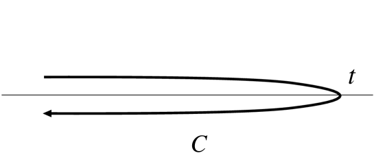
FIG. 1.: Path in the complex time plane. $t$ is the time of measurement.

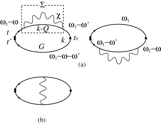
FIG. 2.: Second order contribution to $Q$. (a): Self-energy type. (b): Vertex correction type, which vanishes since interaction vertex $V$ does not depend on the momentum transfer.

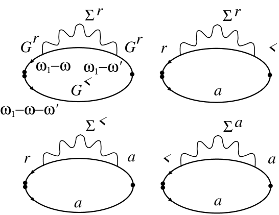
FIG. 3.: Decomposition of $Q^{<}$ into retarded ($r$), advanced ($a$) and lesser components ($<$).

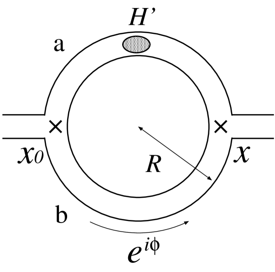
FIG. 4.: Ring we consider. TLS affects only the upper arm (a) and the phase due to magnetic flux ($\phi$) is attached only on the lower arm, b.

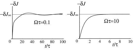
FIG. 5.: Behavior of the current, eq. (61) for the two cases ${\tilde{\Omega}}=0.1$ and ${\tilde{\Omega}}=10$. $u$ and $v$ are chosen as 1.

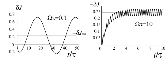
FIG. 6.: Behavior of $|\delta J|\equiv|J(t)-J_{0}|$ for the oscillating external field (eq. (73)), plotted in unit of $2\pi J_{0}N(0)\tau v^{2}$. At $t\rightarrow\infty$ the oscillation is around $|\delta J|=1/4\times 2\pi J_{0}N(0)\tau v^{2}$.

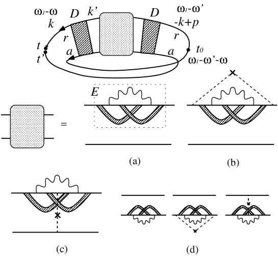
FIG. 7.: Corrections by TLS to AAS oscillation. Shaded thick line denotes Cooperon. Scattering by normal impurity is indicated by a dotted line.

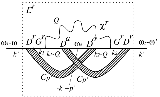
FIG. 8.: Diagrammatic representation of $E^{r}$.

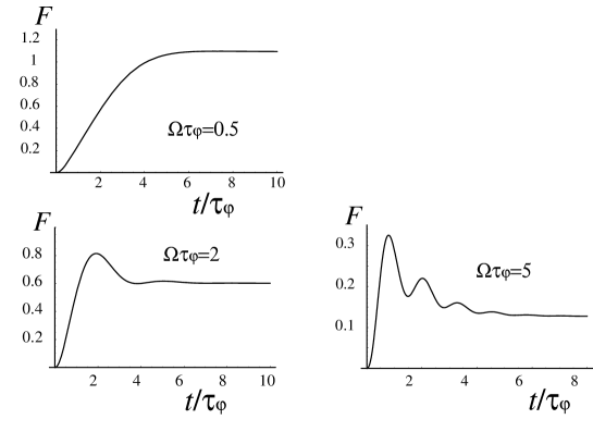
FIG. 9.: Relaxation of the amplitude of AAS oscillation ($F$ of eq. (107)) after switching of TLS for $\Omega\tau_{\varphi}=0.5,2,5$. For $\Omega\tau_{\varphi}\ll 1$ behavior is monotonic, but for $\Omega\tau_{\varphi}\gtrsim 1$, a bump appears in the timescale of $\sim\tau_{\varphi}$ and then a decay.

- [1] A. O. Caldeira and A. J. Leggett, Phys. Rev. Lett. 46, 211 (1981); A. O. Caldeira and A. J. Leggett, Ann. Phys. 149 374, (1983).
- [2] G. Bergmann, Phys. Reports 107, 1 (1984).
- [3] P. A. Lee and T. V. Ramakrishnan, Rev. Mod. Phys. 57, 287 (1985).
- [4] B. L. Altshuler, A. G. Aronov and D. E. Khmelnitsky, J. Phys. C: Sol. St. Phys. 15, 7367 (1982).
- [5] H. Fukuyama and E. Abrahams, Phys. Rev. B27, 5976 (1983).
- [6] A. Stern, Y. Aharonov and Y. Imry, Phys. Rev. A40, 3436 (1990).
- [7] Y. Imry, “Introduction to Mesoscopic Physics”, Oxford University Press (1997).
- [8] Y. Imry, H. Fukuyama and P. Schwab, Europhys. Lett. 47, 608 (1999).
- [9] K.-H. Ahn and P. Mohanty, Phys. Rev. B63, 195301 (2001).
- [10] I. L. Aleiner, B. L. Altshuler and Y. M. Galperin, Phys. Rev. B63, 201401(R) (2001).
- [11] P. Mohanty, E. M. Q. Jariwala and R. A. Webb, Phys. Rev. Lett. 78, 3366 (1997).
- [12] Y. Aharonov and D. Bohm, Phys. Rev. 115, 485 (1959).
- [13] B. L. Altshuler, A. G. Aronov and B. Z. Spivak, Pis’ma Zh. Eksp. Teor. Fiz. 33, 101 (1981) [JETP Lett. 33, 94 (1981)].
- [14] A. G. Aronov and Yu. V. Sharvin, Rev. Mod. Phys. 59, 755 (1987).
- [15] A. Yacoby, M. Heiblum, D. Mahalu and H. Shtrikman, Phys. Rev. Lett. 74, 4047 (1995).
- [16] A. Yacoby, R. Schuster and M. Heiblum, Phys. Rev. B53, 9583 (1996).
- [17] G. Hackenbroich and H. A. Weidenmüller, Phys. Rev. Lett. 76, 110 (1996).
- [18] R. Schuster, E. Buks, M. Heiblum, D. Mahalu, V. Umansky and H. Shtrikman, Nature 385, 417 (1997).
- [19] A. P. Jauho and N. S. Wingreen, Phys. Rev. B58, 9619 (1998).
- [20] K. Yakubo and J. Ohe, J. Phys. Soc. Jpn. 69, 2170 (2000).
- [21] S. Pedersen, A. E. Hansen, A. Krisensen, C. B. Sorensen and P. E. Lindelof, Phys. Rev. B61, 5457 (2000).
- [22] A. E. Hansen, A. Krisensen, S. Pedersen, C. B. Sorensen and P. E. Lindelof, Phys. Rev. B64, 245313 (2001).
- [23] G. Seelig and M. Büttiker, Phys. Rev. B64, 045327 (2001).
- [24] S. Q. Murphy, J. P. Eisenstein, L. N. Pfeiffer and K. W. West, Phys. Rev. B52, 14825 (1995).
- [25] M. C. Beard, G. M. Turner and C. A. Schmuttenmaer, Phys. Rev. B62, 15764 (2000).
- [26] L. V. Keldish, Zh. Eksp. Teor. Fiz. 47, 1515 (1964) [Sov. Phys. - JETP 20, 1018 (1965)].
- [27] H. Haug and A. -P. Jauho, Quantum Kinetics in Transport and Optics of Semi-conductors, (Springer-Verlag, 1998).
- [28] J. Rammer and H. Smith, Rev. Mod. Phys. 58, 323 (1986).
- [29] N. Garcia, M. Munoz and Y. W. Zhao: Phys. Rev. Lett. 82 (1999) 2923.
- [30] G. Tatara, Y.-W. Zhao, M. Muñoz and N. García: Phys. Rev. Lett. 83 (1999) 2030.
- [31] J. I. Versluijs, M. A. Bari and J. M. D. Coey, Phys. rev. Lett. 87, 026601 (2001).
- [32] H. Fukuyama, Prog. Theor. Phys. Suppl. 84, 47 (1985).