Large-scale topological and dynamical properties of Internet

Abstract

We study the large-scale topological and dynamical properties of real Internet maps at the autonomous system level, collected in a three years time interval. We find that the connectivity structure of the Internet presents average quantities and statistical distributions settled in a well-defined stationary state. The large-scale properties are characterized by a scale-free topology consistent with previous observations. Correlation functions and clustering coefficients exhibit a remarkable structure due to the underlying hierarchical organization of the Internet. The study of the Internet time evolution shows a growth dynamics with aging features typical of recently proposed growing network models. We compare the properties of growing network models with the present real Internet data analysis.

I Introduction

The Internet is a capital example of growing complex network Strogatz (2001); Amaral et al. (2000) interconnecting millions of computers around the world. Growing networks exhibit a high degree of wiring entanglement which takes place during their dynamical evolution. This feature, at the heart of the new and interesting topological properties recently observed in growing network systems Albert and Barabási (2001); Dorogovtsev and Mendes (2001a), has triggered the attention of the research community to the study of the large-scale properties of router-level maps of the Internet nla ; cai ; luc . The statistical analysis performed so far has focused on several quantities exhibiting non-trivial properties: wiring redundancy and clustering, Govindan and Reddy (1997); Pansiot and Grad (1998); Faloutsos et al. (1999); Chou (2000), the distribution of chemical distances nla ; Faloutsos et al. (1999), and the eigenvalue spectra of the connectivity matrix Faloutsos et al. (1999). Noteworthy, the presence of a power-law connectivity distribution Govindan and Reddy (1997); Faloutsos et al. (1999); Chou (2000); Caldarelli et al. (2000); Yook et al. (2001) makes the Internet an example of the recently identified class of scale-free networks Barabási and Albert (1999); Barabási et al. (1999). This evidence implies the absence of any characteristic connectivity—large connectivity fluctuations—and a high heterogeneity of the network structure.

As widely pointed out in the literature Doar and Leslie (1993); Floyd and Paxson (2001); Yook et al. (2001), a deeper empirical understanding of the topological properties of Internet is fundamental in the developing of realistic Internet map generators, that on their turn are used to test and optimize Internet protocols. In fact, the Internet topology has a great influence on the dynamics that data traffic carries out on top of it. Hence, a better understanding of the Internet structure is of primary importance in the design of new routing Doar and Leslie (1993); Floyd and Paxson (2001) and searching algorithms Adamic et al. (2001); Puniyani et al. (2001), and to protect from virus spreading Pastor-Satorras and Vespignani (2001) and node failures Albert et al. (2000); Callaway et al. (2000); Cohen et al. (2001). In this perspective, the direct measurement and statistical characterization of real Internet maps are of crucial importance in the identification of the basic mechanisms that rule the Internet structure and dynamics.

In this work, we shall consider the evolution of real Internet maps from 1997 to 2000, collected by the National Laboratory for Applied Network Research (NLANR) nla , in order to study the underlying dynamical processes leading to the Internet structure and topology. We provide a statistical analysis of several average properties. In particular, we consider the average connectivity, clustering coefficient, chemical distance, and betweenness. These quantities will provide a preliminary test of the stationarity of the network. The scale-free nature of the Internet has been pointed out by inspecting the connectivity probability distribution, and it implies that the fluctuations around the average connectivity are not bounded. In order to provide a full characterization of the scale-free properties of the Internet, we analyze the connectivity and betweenness probability distributions for different time snapshot of the Internet maps. We observe that these distributions exhibit an algebraic behavior and are characterized by scaling exponents which are stationary in time. The chemical distance between pairs of nodes, on the other hand, appears to be sharply peaked around its average value, providing a striking evidence for the presence of well-defined small-world properties Watts and Strogatz (1998). A more detailed picture of the Internet can be achieved by studying higher order correlation functions of the network. In this sense, we show that the Internet hierarchical structure is reflected in non-trivial scale-free betweenness and connectivity correlation functions. Finally, we study several quantities related to the growth dynamics of the network. The analysis points out the presence of two distinct wiring processes: the first concerns newly added nodes, while the second is related to already existing nodes increasing their interconnections. We confirm that newly added nodes establish new links with the linear preferential attachment rule often used in modeling growing networks Barabási and Albert (1999). In addition, a study of the connectivity evolution of a single node shows a rich dynamical behavior with aging properties. The present study could provide some hints for a more realistic modeling of the Internet evolution, and with this purpose in mind we provide a discussion of some of the existing growing network models in the light of our findings. A short account of these results appeared in Ref. Pastor-Satorras et al. (2001).

The paper is organized as follows. In Section II we describe the Internet maps used in our study. Sec. III is devoted to the study of average quantities as a function of time. In Sec. IV we provide the analysis of the statistical distributions characterizing the Internet topology. We obtain evidence for the scale-free nature of this network as well as for the stationarity in time of this property. In Sec. V we characterize the hierarchical structure of the Internet by the statistical analysis of the betweenness and connectivity correlation functions. Sec. VI reports the study of dynamical properties such as the preferential attachment and the evolution of the average connectivity of newly added nodes. These properties, which show aging features, are the basis for the developing of Internet dynamical models. Sec. VII is devoted to a detailed discussion of some Internet models as compared with the presented real data analysis. Finally, in Sec. VIII we draw our conclusions and perspectives.

II Mapping the Internet

Several Internet mapping projects are currently devoted to obtain high-quality router-level maps of the Internet. In most cases, the map is constructed by using a hop-limited probe (such as the UNIX traceroute tool) from a single location in the network. In this case the result is a “directed”, map as seen from a specific location on the Internet luc . This approach does not correspond to a complete map of the Internet because cross-links and other technical problems (such as multiple Internet provider aliases) are not considered. Heuristic methods to take into account these problems have been proposed (see for instance Ref. mer ). However, it is not clear their reliability and the corresponding completeness of the maps constructed this way.

A different representation of Internet is obtained by mapping the autonomous systems (AS) topology. The Internet can be considered as a collection of subnetworks that are connected together. Within each subnetwork the information is routed using an internal algorithm that may differ from one subnetwork to another. Thus, each subnet is an independent unit of the Internet and it is often referred as an AS. These AS communicate between them using a specific routing algorithm, the Border Gateway Protocol. Each AS number approximately maps to an Internet Service Provider (ISP) and their links are inter-ISP connections. In this case it is possible to collect data from several probing stations to obtain complete interconnectivity maps (see Refs. nla ; cai for a technical description of these projects). In particular, the NLANR project is collecting data since Nov. 1997, and it provides topological as well as dynamical information on a consistent subset of the Internet. The first Nov. 1997 map contains 3180 AS, and it has grown in time until the Dec. 1999 measurement, consisting of 6374 AS. In the following we will consider the graph whose nodes represent the AS and whose links represent the adjacencies (interconnections) between AS. In particular we will focus in three different snapshots corresponding to November 8th 1997, 1998, and 1999, that will be referenced as AS97, AS98, and AS99, respectively.

The NLANR connectivity maps are collected with a resolution of one day and are changing from day to day. These changes are due to the addition (birth) and deletion (death) of nodes and links, but also to the flickering of connections, so that a node may appear to be isolated (not mapped) from time to time. A simple test, however, shows that flickering is appreciable just in nodes with low connectivity. We compute the ratio $r$ between the number of days in which a node is observed in the NLANR maps and the total number of days after the first appearance of the node, averaged over all nodes in the maps. The analysis reveals that $r\simeq 1$ and $r>0.65$ for nodes with connectivity $k\geq 10$, and $k<10$, respectively. Hence, nodes with $k<10$ have fluctuations that must be taken into account. In order to shed light on this point, we inspect the incidence of death events with respect to the creation of new nodes. We consider a death event only if a node is not observed in the map during a one year time interval. In Table 1 we show the total number of death events in a year, for 1997, 1998, and 1999, in comparison with the total number of new nodes created. It can be seen that the AS’s birth rate appears to be larger by a factor of two than the death rate. More interestingly, if we restrict the analysis to nodes with connectivity $k>10$, the death rate is reduced to a few percent of the birth rate. This clearly indicates that only poorly connected nodes have an appreciable probability to disappear. This fact is easily understandable in terms of the market competition among ISP’s, where small newcomers are the ones which more likely go out of business.

Year	1997	1998	1999
$N_{\rm new}$	309	1990	3410
$N_{\rm dead}$	129	887	1713
$N_{\rm dead}(k>10)$	0	14	68

Table 1: Total number of new ($N_{\rm new}$) and deleted ($N_{\rm dead}$) nodes in the years 1997, 1998, and 1999. We also report the number of deleted nodes with connectivity $k>10$.

III Average properties and stationarity

The growth rate of AS maps reveals that the Internet is a rapidly evolving network. Thus, it is extremely important to know whether or not it has reached a stationary state whose average properties are time-independent. This will imply that, despite the continuous increase of nodes and connections in the system, the network’s topological properties are not appreciably changing in time. As a first step, we have analyzed the behavior in time of several average magnitudes: the average connectivity $\left<k\right>$, the clustering coefficient $\left<c\right>$, the average chemical distance $\left<d\right>$, and the average betweenness $\left<b\right>$.

The connectivity $k_{i}$ of a node $i$ is defined as the number of connections of this node with other nodes in the network, and $\left<k\right>$ is the average of $k_{i}$ over all nodes in the network. Since each connection contributes to the connectivity of two nodes, we have that $\left<k\right>=2E/N$, where $E$ is the total number of connections and $N$ is the number of nodes. Both $E$ and $N$ are increasing with time but their ratio remains almost constant. The average connectivity for the 1997, 1998, and 1999 years (averaged over all the AS maps available for that year) is shown in Table 2. In average each node has three to four connections, which is a small number compared with that of a fully connected network of the same size ($\left<k\right>=N-1\sim 10^{3}$). The average connectivity gives information about the number of connections of any node but not about the overall structure of these connections. More information can be obtained using the clustering coefficient introduced in Ref. Watts and Strogatz (1998). The number of neighbors of a node $i$ is given by its connectivity $k_{i}$. On their turn, these neighbors can be connected among them forming a triangle with node $i$. The clustering coefficient $c_{i}$ is then defined as the ratio between the number of connections among the $k_{i}$ neighbors of a given node $i$ and its maximum possible value, $k_{i}(k_{i}-1)/2$. The average clustering coefficient $\left<c\right>$ is the average of $c_{i}$ over all nodes in the network. The clustering coefficient thus provides a measure of how well locally interconnected are the neighbors of any node. The maximum value of $\left<c\right>$ is 1, corresponding to a fully connected network. For random graphs Bollobás (1985), which are constructed by connecting nodes at random with a fixed probability $p$, the clustering coefficient decreases with the network size $N$ as $\left<c\right>_{\rm rand}=\left<k\right>/N$. On the contrary, it remains constant for regular lattices. The average clustering coefficient obtained for the 1997, 1998, and 1999 years is shown in Table 2. As it can be seen, the clustering coefficient of the AS maps increases slowly with increasing $N$ and takes values $\left<c\right>\simeq 0.2$, two orders of magnitudes larger than $\left<c\right>_{\rm rand}\simeq 10^{-3}$, corresponding to a random graph with the same number of nodes. Therefore, the AS maps are far from being a random graph, a feature that can be naively understood using the following argument: In AS maps the connections among nodes are equivalent, but they are actually characterized by a real space length corresponding to the actual length of the physical connection between AS. The larger is this length, the higher the costs of installation and maintenance of the line, favoring therefore the connection between nearby nodes. It is thus likely that nodes within the same geographical region will have a large number of connection among them, increasing in this way the local clustering coefficient.

Year	1997	1998	1999
$N$	3112	3834	5287
$E$	5450	6990	10100
$\left\langle k\right\rangle$	3.5(1)	3.6(1)	3.8(1)
$\left\langle c\right\rangle$	0.18(3)	0.21(3)	0.24(3)
$\left\langle d\right\rangle$	3.8(1)	3.8(1)	3.7(1)
$\left\langle b\right\rangle/N$	2.4(1)	2.3(1)	2.2(1)

Table 2: Average properties of the Internet for three different years. $N$: number of nodes; $E$: number of connections; $\left\langle k\right\rangle$: average connectivity; $\left\langle c\right\rangle$: average clustering coefficient; $\left\langle d\right\rangle$ average chemical distance; $\left\langle b\right\rangle$ average betweenness. Figures in parenthesis indicate the statistical uncertainty from averaging the values of the corresponding months in each year.

With this reasoning one might be lead to the conclusion that the Internet topology is close to a regular two-dimensional lattice. The analysis of the chemical distances between nodes, however, reveals that this is not the case. Two nodes $i$ and $j$ are said to be connected if one can go from node $i$ to $j$ following the connections in the network. The path from $i$ to $j$ may be not unique and its distance is given by the number of nodes visited. The average chemical distance $\left<d\right>$ is defined as the shortest path distance between two nodes $i$ and $j$, $d_{ij}$, averaged over every pair of nodes in the network. For regular lattices, $\left<d\right>_{D}\sim N^{1/D}$, where $D$ is the spatial dimension. Hence, if the Internet could be mapped into a two-dimensional lattice, we should observe $\left<d\right>_{\rm D=2}\sim N^{1/2}\approx 60$. However, as it can be seen from Table 2, for the AS maps $\left<d\right>\simeq 3.6\ll\left<d\right>_{\rm D=2}$. The Internet strikingly exhibits what is known as the “small-world” effect Watts and Strogatz (1998); Watts (1999): in average one can go from one node to any other in the system passing through a very small number of intermediate nodes. This necessarily implies that besides the short local connections which contribute to the large clustering coefficient, there are some hubs and backbones which connect different regional networks, strongly decreasing the average chemical distance. Another measure of this feature is given by the number of minimal paths that pass by each node. To go from one node in the network to another following the shortest path, a sequence of nodes is visited. If we do this for every pair of nodes in the network, there will be a certain number of key nodes that will be visited more often than others. Such nodes will be of great importance for the transmission of information along the network. This fact can be quantitatively measured by means of the betweenness $b_{i}$, defined by the total number of shortest paths between any two nodes in the network that pass thorough the node $i$. The average betweenness $\left<b\right>$ is the average value of $b_{i}$ over all nodes in the network. The betweenness has been introduced in the analysis of social network in Ref. Newman (2001) and more recently it has been studied in scale-free networks, with the name of load Goh et al. (2001). Moreover, an algorithm to compute the betweenness has been given in Ref. Newman (2001). For a star network the betweenness takes its maximum value $N(N-1)/2$ at the central node and its minimum value $N-1$ at the vertices of the star. The average betweenness of the three AS maps analyzed here is shown in Table 2. Its value is between $2N$ and $3N$, which is quite small in comparison with its maximum possible value $N(N-1)\sim 10^{7}$.

The present analysis makes clear that the Internet is not dominated by a very few highly connected nodes similarly to star-shaped architectures. As well, simple average measurements rule out the possibility of a random graph structure or a regular grid architecture. This evidence hints towards a peculiar topology that will be fully identified by looking at the detailed probability distributions of several quantities. Finally, it is important to stress that despite the network size is more than doubled in the three years period considered, the average quantities suffer variations of a few percent (see Table 2). This points out that the system seems to have reached a fairly well-defined stationary state, as we shall confirm in the next Section by analyzing the detailed statistical properties of the Internet.

IV Fluctuations and scale-free properties

In order to get a deeper understanding of the network topology we look at the probability distributions $p_{k}(k)$ and $p_{b}(b)$ that any given node in the network has a connectivity $k$ and a betweenness $b$, respectively. The study of these probability distributions will allow us to probe the extent of fluctuations and heterogeneity present in the network. We shall see that the strong scale-free nature of the Internet, previously noted in Refs. Faloutsos et al. (1999); Caldarelli et al. (2000), results in power-law distributions with diverging fluctuations for these quantities. The analysis of the maps reveals, in fact, an algebraic decay for the connectivity distribution,

$$p_{k}(k)\sim k^{-\gamma},$$ (1)

extending over three orders of magnitude. In Fig. 1 we report the integrated connectivity distribution

$$P_{k}(k)=\int_{k}^{\infty}p_{k}(k^{\prime})dk^{\prime}$$ (2)

corresponding to the AS97, AS98, and AS99 maps. The integrated distribution, which expresses the probability that a node has connectivity larger than or equal to $k$, scales as

$$P_{k}(k)\sim k^{1-\gamma},$$ (3)

and it has the advantage of being considerably less noisy that the original distribution. In all maps we find a clear power-law behavior with slope close to $-1.2$ (see Fig. 1), yielding a connectivity exponent $\gamma=2.2\pm 0.1$. The distribution cut-off is fixed by the maximum connectivity of the system and is related to the overall size of the Internet map. We see that for more recent maps the cut-off is slightly increasing, as expected due to the Internet growth. On the other hand, the connectivity exponent $\gamma$ seems to be independent of time and in good agreement with previous measurements Faloutsos et al. (1999).

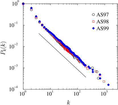
Figure 1: Integrated connectivity distribution for the AS97, AS98, and AS99 maps. The power-law behavior is characterized by a slope $-1.2$, which yields a connectivity exponent $\gamma=2.2\pm 0.1$.

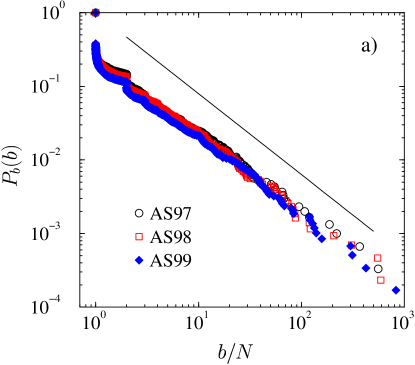
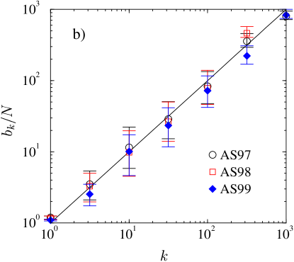
Figure 2: a) Integrated betweenness distribution for the AS97, AS98, and AS99 maps. The power-law behavior is characterized by a slope $-1.1$, which yields a betweenness exponent $\delta=2.1\pm 0.2$. b) Betweenness $b_{k}$ as a function of the node’s connectivity $k$. The full line corresponds to the predicted behavior $b_{k}\sim k$. Errors bars take into account statistical fluctuations over different nodes with the same connectivity.

The betweenness distribution $p_{b}(b)$ (i.e. the probability that any given node is passed over by $b$ shortest paths) shows also scale-free properties, with a a power-law distribution

$$p_{b}(b)\sim b^{-\delta}$$ (4)

extending over three decades. As shown in Fig. 2(a), the integrated betweenness distribution measured in the AS maps is evidently stable in the three years period analyzed and follows a power-law decay

$$P_{b}(b)=\int_{b}^{\infty}p_{b}(b^{\prime})db^{\prime}\sim b^{1-\delta},$$ (5)

where the betweenness exponent is $\delta=2.1\pm 0.2$. The connectivity and betweenness exponents can be simply related if one assumes that the number of shortest paths $b_{k}$ passing over a node of connectivity $k$ follows the scaling form

$$b_{k}\sim k^{\beta}.$$ (6)

By inserting the latter relation in the integrated betweenness distribution Eq. (5) we obtain

$$P_{k}(k)\sim k^{\beta(1-\delta)}.$$ (7)

Since we have that $P_{k}(k)\sim k^{1-\gamma}$, we obtain the scaling relation

$$\beta=\frac{\gamma-1}{\delta-1}.$$ (8)

The measured $\gamma$ and $\delta$ have approximately the same value for the AS maps data and we expect to recover $\beta\approx 1.0$. This is corroborated in Fig. 2(b), where we report the direct measurement of the average betweenness of a node as a function of its connectivity $k$. It is also worth remarking that it has been recently argued Goh et al. (2001) that the betweenness distribution of scale-free networks with $2<\gamma\leq 3$ is an universal quantity not depending on $\gamma$. From a numerical study of two scale-free network models Goh et al. (2001), it was found that the betweenness distribution follows a universal power-law decay with an exponent $\delta\approx 2.2$, in fair agreement with our findings.

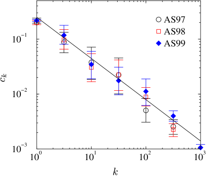
Figure 3: Clustering coefficient $c_{k}$ as a function of the connectivity $k$ for the AS97, AS98, and AS99 maps. The best fitting power-law behavior is characterized by a slope $-0.75$.Errors bars take into account statistical fluctuations over different nodes with the same connectivity.

Another quantity of interest is the probability distribution of the clustering coefficient of the nodes. In our analysis we don’t find definitive evidence for a power-law behavior of this distribution. However, still useful information can be gathered from studying the clustering coefficient $c_{k}$ as a function of the node connectivity. In this case the local clustering coefficient of each node $c_{i}$ is averaged over all nodes with the same connectivity $k$. The plots for the AS97, AS98 and AS99 maps are shown in Fig. 3. Also in this case, measurements yield a power-law behavior $c_{k}\sim k^{-\omega}$ with $\omega=0.75\pm 0.03$, extending over three orders of magnitudes. This implies that nodes with a small number of connections have larger local clustering coefficients than those with a large connectivity. This behavior is consistent with the picture previously described in Sec. III of highly clustered regional networks sparsely interconnected by national backbones and international connections. The regional clusters of AS are probably formed by a large number of nodes with small connectivity but large clustering coefficients. Moreover, they also should contain nodes with large connectivities that are connected with the other regional clusters. These large connectivity nodes will be on their turn connected to nodes in different clusters which are not interconnected and, therefore, will have a small local clustering coefficient. This picture also shows the existence of some hierarchy in the network that will become more evident in the next Section.

     

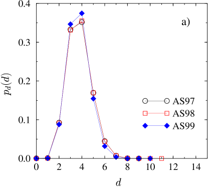
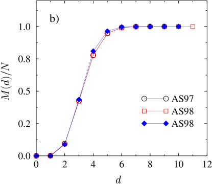
Figure 4: a) Distribution of chemical distances $p_{d}(d)$ for the AS97, AS98, and AS99 maps. b) Hop plots $M(d)$ for the same maps. See text for definitions.

A different behavior is followed by the chemical distance $d$ between two nodes, which does not show singular fluctuations from one pair of nodes to another. This can be shown by means of the probability distribution $p_{d}(d)$ of chemical distances $d$ between pairs of nodes, reported in Fig. 4(a). This distribution is characterized by a sharp peak around its average value and its shape remains essentially unchanged from the AS97 to the AS99 maps. Associated to the chemical distance distribution we have the hop plot introduced in Ref. Faloutsos et al. (1999). The hop plot is defined as the average fraction of nodes $M(d)/N$ within a chemical distance less than or equal to $d$ from a given node. At $d=0$ we find the starting node and, therefore, $M(0)=1$. At $d=1$ we found the starting node plus its neighbors and thus $M(1)=\left<k\right>+1$. If the network is made by a single cluster, for $d=d_{M}$, where $d_{M}$ is the maximum chemical distance, $M(d_{M})=N$. For regular $D$-dimensional lattices, $M(d)\sim d^{D}$, and in this case $M$ can be interpreted as the mass. The hop plot is related to the distribution of chemical distances through the following relation:

$$\frac{M(d)}{N}=\sum_{d^{\prime}=0}^{d}p_{d}(d^{\prime}).$$ (9)

The hop plots for the AS97, AS98 and AS99 maps are shown in Fig. 4(b). In this case the chemical distance barely spans a decade ($d_{M}=11$). Most importantly, $M(d)$ practically reaches its maximum value $N$ at $d=5$. Hence, the chemical distance does not show strong fluctuations, as already noticed from the chemical distance distribution. In Ref. Faloutsos et al. (1999) it was argued that the increase of $M(d)$ for small $d$ follows a power-law distribution. This observation is not consistent with the present data, that yield a very abrupt increase taking place in a very narrow range.

Finally, it is important to stress again that all the measured distributions are characterized by scaling exponents or behaviors which are not changing in time. This implies that the statistical properties characterizing the Internet are time independent, providing a further test to the network stationarity; i.e. the Internet is self-organized in a stationary state characterized by scale-free fluctuations.

V Hierarchy and correlations

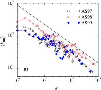
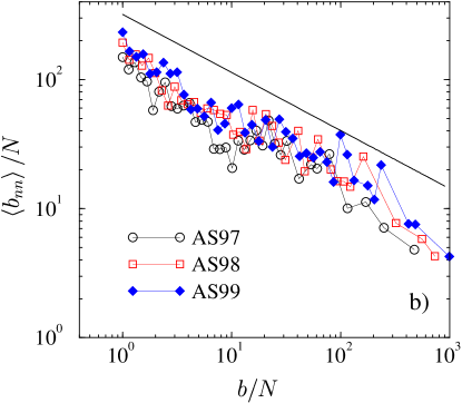
Figure 5: a) Average connectivity $\left<k_{nn}\right>$ of the nearest neighbors of a node as a function of the connectivity $k$ for the same maps. The full line has a slope $-0.5$. b) Average betweenness $\left<b_{nn}\right>$ of the nearest neighbors of a node as a function of its betweenness $b$ for the AS97, AS98, and AS99 maps. The full line has a slope $-0.4$.

Due to installation costs, the Internet has been designed with a hierarchical structure. The primary known structural difference between Internet nodes is the distinction between stub and transit domains. Nodes in stub domains have links that go only through the domain itself. Stub domains, on the other hand, are connected via a gateway node to transit domains that, on the contrary, are fairly well interconnected via many paths. This hierarchy can be schematically divided into international connections, national backbones, regional networks, and local area networks. Nodes providing access to international connections or national backbones are of course on top level of this hierarchy, since they make possible the communication between regional and local area networks. Moreover, in this way, a small average chemical distance can be achieved with a small average connectivity.

Very likely the hierarchical structure will introduce some correlations in the network topology. We can explore the hierarchical structure of the Internet by means of the conditional probability $p_{c}(k^{\prime}|k)$ that a link belonging to node with connectivity $k$ points to a node with connectivity $k^{\prime}$. If this conditional probability is independent of $k$, we are in presence of a topology without any correlation among the nodes’ connectivity. In this case, $p_{c}(k^{\prime}|k)=p_{c}(k^{\prime})\sim k^{\prime}p_{k}(k^{\prime})$, in view of the fact that any link points to nodes with a probability proportional to their connectivity. On the contrary, the explicit dependence on $k$ is a signature of non-trivial correlations among the nodes’ connectivity, and the presence of a hierarchical structure in the network topology. A direct measurement of the $p_{c}(k^{\prime}|k)$ function is a rather complex task due to large statistical fluctuations. More clear indications can be extracted by studying the quantity

$$\left<k_{nn}\right>=\sum_{k^{\prime}}k^{\prime}p_{c}(k^{\prime}|k),$$ (10)

i.e. the nearest neighbors average connectivity of nodes with connectivity $k$. In Fig. 5(a) we show the results obtained for the AS97, AS98, and AS99 maps, that again exhibit a clear power-law dependence on the connectivity degree,

$$\left<k_{nn}\right>\sim k^{-\nu_{k}},$$ (11)

with an exponent $\nu_{k}=0.5\pm 0.1$. This observation clearly implies that the connectivity correlation function has a marked dependence upon $k$, suggesting non-trivial correlation properties for the Internet. In practice, this result indicates that highly connected nodes are more likely pointing to less connected nodes, emphasizing the presence of a hierarchy in which smaller providers connect to larger ones and so on, climbing different levels of connectivity.

Similarly, it is expected that nodes with high betweenness (that is, carrying a heavy load of transit), and consequently a large connectivity, will be connected to nodes with smaller betweenness, less load and, therefore, small connectivity. A simple way to measure this effect is to compute the average betweenness $\left<b_{nn}\right>$ of the neighbors of the nodes with a given betweenness $b$. The plot of $\left<b_{nn}\right>$ for the AS97, AS98, and AS99 maps, represented in Fig. 5(b), shows that the average neighbor betweenness exhibits a clear power-law dependence on the node betweenness $b$,

$$\left<b_{nn}\right>\sim b^{-\nu_{b}},$$ (12)

with an exponent $\nu_{b}=0.4\pm 0.1$, evidencing that the more loaded nodes (backbones) are more frequently connected with less loaded nodes (local networks).

These hierarchical properties of the Internet are likely driven by several additional factors such as the space locality, economical resources and the market demand. An attempt to relate and study some of these aspects can be found in Ref. Yook et al. (2001), where the geographical distribution of population and Internet access are studied. In Sec. VII we shall compare a few of the existing models for the generation of scale-free networks with our data analysis, in an attempt to identify some relevant features in the Internet modeling.

VI Dynamics and growth

In order to inspect the Internet dynamics, we focus our attention on the addition of new nodes and links into the maps. In the three-years range considered, we keep track of the number of links $\ell_{\rm new}$ appearing between a newly introduced node and an already existing node. We also monitor the rate of appearance of links $\ell_{\rm old}$ between already existing nodes. In Table 3 we can observe that the creation of new links is governed by these two processes at the same time. Specifically, the largest contribution to the growth is given by the appearance of links between already existing nodes. This clearly points out that the Internet growth is strongly driven by the need of redundancy in the wiring and an increased need of available bandwidth for data transmission.

Year	1997	1998	1999
$\ell_{\rm new}$	183(9)	170(8)	231(11)
$\ell_{\rm old}$	546(35)	350(9)	450(29)
$\ell_{\rm new}/\ell_{\rm old}$	0.34(2)	0.48(2)	0.53(3)

Table 3: Monthly rate of new links connecting existing nodes to new ($\ell_{\rm new}$) and old ($\ell_{\rm old}$) nodes.

A customarily measured quantity in the case of growing networks is the average connectivity $\left<k_{i}(t)\right>$ of new nodes as a function of their age $t$. In Refs. Barabási et al. (1999); Krapivsky et al. (2000); Krapivsky and Redner (2001) it is shown that $\left<k_{i}(t)\right>$ is a scaling function of both $t$ and the absolute time of birth of the node $t_{0}$. We thus consider the total number of nodes born within an small observation window $\Delta t_{0}$, such that $t_{0}\simeq{\rm const.}$ with respect to the absolute time scale that is the Internet lifetime. For these nodes, we measure the average connectivity as a function of the time $t$ elapsed since their birth. The data for two different time windows are reported in Fig. 6, where it is possible to distinguish two different dynamical regimes: At early times, the connectivity is nearly constant with a very slow increase ($\left<k_{i}(t)\right>\sim t^{0.1}$). Later on, the behavior approaches a power-law growth $\left<k_{i}(t)\right>\sim t^{0.5}$. While exponent estimates are affected by noise and limited time window effects, the crossover between two distinct dynamical regimes is compatible with the general aging form obtained in the context of growing networks in Ref. Krapivsky et al. (2000); Krapivsky and Redner (2001).

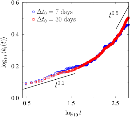
Figure 6: Average connectivity of nodes borne within a small time window $\Delta t_{0}$, after a time $t$ elapsed since their appearance. Time $t$ is measured in days. As a comparison we report the lines corresponding to $t^{0.1}$ and $t^{0.5}$.

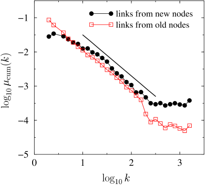
Figure 7: Integrated frequency of links emanating from new and existing nodes that attach to nodes with connectivity $k$. The full line corresponds to a slope $-0.2$, which yields an exponent $\alpha\simeq 1.0$. The flat tails are originated from the poor statistics at very high $k$ values.

A very important issue in the modeling of growing networks concerns the understanding of the growth mechanisms at the origin of the developing of new links. As we shall see more in detail in the next Section, the basic ingredients in the modeling of scale-free growing networks is the preferential attachment hypothesis Barabási and Albert (1999). In general, all growing network algorithms define models in which the rate $\Pi(k)$ with which a node with $k$ connections receives new links is proportional to $k^{\alpha}$ (see Ref. Barabási and Albert (1999) and Sec. VII). The inspection of the exact value of $\alpha$ in real networks is an important issue since the connectivity properties strongly depend on this exponent Krapivsky et al. (2000); Krapivsky and Redner (2001); Jeong et al. (2001). Here we use a simple recipe that allows to extract the value of $\alpha$ by studying the appearance of new links. We focus on links emanating from newly appeared nodes in different time windows ranging from one to three years. We consider the frequency $\mu(k)$ of links that connect to nodes with connectivity $k$. By using the preferential attachment hypothesis, this effective probability is $\mu(k)\sim k^{\alpha}p_{k}(k)$. Since we know that $p_{k}(k)\sim k^{-\gamma}$, we expect to find a power-law behavior $\mu(k)\sim k^{\alpha-\gamma}$ for the frequency. In Fig. 7 we report the obtained results for the integrated frequency $\mu_{\rm cum}(k)=\int_{k}^{\infty}\mu(k^{\prime})dk^{\prime}$, which shows a behavior compatible with an algebraic dependence $\mu(k)\sim k^{-1.2}$. By using the independently obtained value $\gamma=2.2$ we find a preferential attachment exponent $\alpha\simeq 1.0$, in good agreement with the result obtained with a different analysis in Ref. Jeong et al. (2001). We performed a similar analysis also for links emanated by existing nodes, recovering the same form of preferential attachment (see Fig. 7). The present analysis confirms the validity of the preferential attachment hypothesis, but leaves open the question of the interplay with several other factors, such as the nodes’ hierarchy, space locality, and resource constraints.

VII Modeling the Internet

In the previous Section we have presented a thorough analysis of the AS maps topology. Apart from providing useful empirical data to understand the behavior of the Internet, our analysis is of great relevance in order to test the validity of models of the Internet topology. The Internet topology has a great influence on the information traffic carried on top of it, including routing algorithms Doar and Leslie (1993); Floyd and Paxson (2001), searching algorithms Adamic et al. (2001); Puniyani et al. (2001), virus spreading Pastor-Satorras and Vespignani (2001), and resilience to node failure Albert et al. (2000); Callaway et al. (2000); Cohen et al. (2001). Thus, designing network models which accurately reproduce the Internet topology is of capital importance to carry out simulations on top of these networks.

Early works considered the Erdös-Rényi Erdös and Rényi (1960) model or hierarchical networks as models of Internet Zegura et al. (1997). However, they yield connectivity distributions with a fast (exponential) decay for large connectivities, in disagreement with the power-law decay observed in real data. Only recently the Internet modeling benefited of the major advance provided in the field of growing networks by the introduction of the Barabási-Albert (BA) model Barabási and Albert (1999); Barabási et al. (1999); Dorogovtsev et al. (2000a), which is related to 1955 Simon’s model Simon (1955); Bornholdt and Ebel (2001); Dorogovtsev et al. (2000b). The main ingredients of this model are the growing nature of the network and a preferential attachment rule, in which the probability of establishing new links toward a given node grows linearly with its connectivity. The BA model is constructed using the following algorithm Barabási and Albert (1999): We start from a small number $m_{0}$ of disconnected nodes; every time step a new node is added, with $m$ links that are connected to an old node $i$ with probability

$$\Pi_{\rm BA}(k_{i})=\frac{k_{i}}{\sum_{j}k_{j}},$$ (13)

where $k_{i}$ is the connectivity of the $i$-th node. After iterating this procedure $N$ times, we obtain a network with a connectivity distribution $p_{k}(k)\sim k^{-3}$ and average connectivity $\left<k\right>=2m$. In this model, heavily connected nodes will increase their connectivity at a larger rate than less connected nodes, a phenomenon that is known as the “rich-get-richer” effect Barabási and Albert (1999). It is worth remarking, however, that more general studies Krapivsky et al. (2000); Krapivsky and Redner (2001); Dorogovtsev and Mendes (2001a) have revealed that nonlinear attachment rates of the form $\Pi(k)\sim k^{\alpha}$ with $\alpha\neq 1$ have as an outcome connectivity distributions that depart form the power-law behavior. The BA model has been successively modified with the introduction of several ingredients in order to account for connectivity distribution with $2<\gamma<3$ Albert and Barabási (2000); Krapivsky et al. (2000); Krapivsky and Redner (2001), local geographical factors Medina et al. (2000), wiring among existing nodes Dorogovtsev and Mendes (2000), and age effects Dorogovtsev and Mendes (2001b).

In the previous Section we have analyzed different measures that characterize the structure of AS maps. Since several models are able to reproduce the right power law behavior for the connectivity distribution, the analysis obtained in the previous sections can provide the effective tools to scrutinize the different models at a deeper level. In particular, we perform a data comparison for three different models that generate networks with power-law connectivity distributions. First we have considered a random graph constructed with a power-law connectivity distribution, using the Molloy and Reed (MR) algorithm Molloy and Reed (1995, 1998). Secondly, we have studied two variations of the BA model, that yield connectivity exponents compatible with the one measured in Internet: the generalized Barabási-Albert (GBA) model Albert and Barabási (2000), which includes the possibility of connection rewiring, and the fitness model Bianconi and Barabási (2001), that implements a weighting of the nodes in the preferential attachment probability.

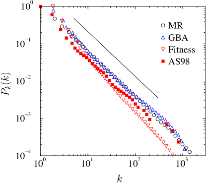
Figure 8: Integrated connectivity distribution for the MR, GBA, and fitness models, compared with the result from the AS98 map. The full line has slope $-1.2$.

The models are defined as follows:

MR model: In the construction of this model Molloy and Reed (1995, 1998); Newman et al. (2001); Dorogovtsev and Mendes (2001a) we start assigning to each node $i$ in a set of $N$ nodes a random connectivity $k_{i}$ drawn from the probability distribution $p_{k}(k)\sim k^{-\gamma}$, with $m\leq k_{i}<N$, and imposing the constraint that the sum $\sum_{i}k_{i}$ must be even. The graph is completed by randomly connecting the nodes with $\sum_{i}k_{i}/2$ links, respecting the assigned connectivities. The results presented here are obtained using $m=1$ and a connectivity exponent $\gamma=2.2$, equal to that found in the AS maps. Clearly this construction algorithm does not take into account any correlations or dynamical feature of the Internet and it can be considered as a first order approximations that focuses only in the connectivity properties.

GBA model: It is defined by starting with $m_{0}$ nodes connected in a ring Albert and Barabási (2000): At each time step one of the following operations is performed:

• With probability $q$ we rewire $m$ links. For each of them, we randomly select a node $i$ and a link $l_{ij}$ connected to it. This link is removed and replaced by a new link $l_{i^{\prime}j}$ connecting the node $j$ to a new node $i^{\prime}$ selected with probability $\Pi(k_{i^{\prime}})$ where

  $$\Pi_{\rm GBA}(k_{i})=\frac{k_{i}+1}{\sum_{j}(k_{j}+1)}.$$ (14)

• With probability $p$ we add $m$ new links. For each of them, one end of the link is selected at random, while the other is selected with probability as in Eq. (14).

• With probability $1-q-p$ we add a new node with $m$ links that are connected to nodes already present with probability as in Eq. (14).

The preferential attachment probability Eq. (14) leads to a power-law distributed connectivity, whose exponent depends on the parameters $q$ and $p$. In the particular case $p=0$, the connectivity exponent is given by Albert and Barabási (2000)

$$\gamma=1+\frac{(1-q)(2m+1)}{m}.$$ (15)

Hence, changing the value of $m$ and $q$ we can obtain the desired connectivity exponent $\gamma$. In the present simulations we use the values $m=2$ and $q=13/25$, that yield the exponent $\gamma=2.2$. The GBA model embeds both the rich-get-richer paradigm and the growing nature of the Internet; however, it does not take into account any possible difference or hierarchies in newly appearing nodes.

Fitness model: This network model introduces an external competence among nodes to gain links, that is controlled by a random (fixed) fitness parameter $\eta_{i}$ that is assigned to each node $i$ from a probability distribution $\rho(\eta)$. In this case, we also start with $m_{0}$ nodes connected in a ring and at each time step we add a new node $i^{\prime}$ with $m$ links that are connected to nodes already present on the network with probability

$$\Pi_{\rm fitness}(k_{i})=\frac{\eta_{i}k_{i}}{\sum_{j}\eta_{j}k_{j}}.$$ (16)

The newly added node is assigned a fitness $\eta_{i^{\prime}}$. The results presented here are obtained using $m=2$ and a probability $\rho(\eta)$ uniformly distributed in the interval $[0,1]$, which yields a connectivity distribution $p_{k}(k)\sim k^{-\gamma}/\ln k$ with $\gamma\approx 2.26$ Bianconi and Barabási (2001). The fitness model adds to the growing dynamics with preferential attachment a stochastic parameter, the fitness, that embeds all the properties, other than the connectivity, that may influence the probability of gaining new links.

	MR	GBA	Fitness	1998
$\left\langle k\right\rangle$	4.8(1)	5.4(1)	4.00(1)	3.6(1)
$\left\langle c\right\rangle$	0.16(1)	0.12(1)	0.02(1)	0.21(3)
$\left\langle d\right\rangle$	3.1(1)	1.8(1)	4.0(1)	3.8(1)
$\left\langle b\right\rangle/N$	2.2(1)	1.9(1)	2.1(1)	2.3(1)

Table 4: Average properties of the MR, GBA, and fitness models, compared with the values from the Internet in 1998. $\left\langle k\right\rangle$: average connectivity; $\left\langle c\right\rangle$: average clustering coefficient; $\left\langle d\right\rangle$ average chemical distance; $\left\langle b\right\rangle$ average betweenness. Figures in parenthesis indicate the statistical uncertainty from the average of $1000$ realizations of the models.

We have performed simulations of these three models using the parameters mentioned above and using sizes of $N\simeq 4000$ nodes, in analogy with the size of the AS map analyzed. In each case we perform averages over $1000$ different realizations of the networks. It is worth remarking that while the fitness model generates a connected network, both the GBA and the MR model yield disconnected networks. This is due to the rewiring process in the GBA model, while the disconnect nature of the graph in the MR model is an inherent consequence of the connectivity exponent being larger that $2$ Newman et al. (2001). In these two cases we therefore work with graphs whose giant component (that is, the largest cluster of connected nodes in the network Bollobás (1985)) has a size of the order $N$. It is important to remind the reader that we are working with networks of a relatively small size, chosen so as to fit the size of the Internet maps analyzed in the previous Sections. In this perspective, all the numerical analysis that we shall perform in the following serve only to check the validity of the models as representations of the Internet as we know it, and do not refer to the intrinsic properties of the models in the thermodynamic limit $N\to\infty$.

As a first check of the connectivity properties of the models, in Fig 8 we have plotted the integrated connectivity distributions. For the MR model we recover the expected exponent $\gamma_{\rm MR}\simeq 2.20$, since it was imposed in the very definition of the model. For the GBA model we obtain numerically $\gamma_{\rm GBA}\simeq 2.19$ for the giant component, in excellent agreement with the value predicted by Eq. (15) for the asymptotic network. For the fitness model, on the other hand, a numerical regression of the integrated connectivity distribution yields an effective exponent $\gamma_{\rm fitness}\simeq 2.4$. This value is larger than the theoretical prediction $2.26$ obtained for the model Bianconi and Barabási (2001). The discrepancy is mainly due to the logarithmic corrections present in the connectivity distribution of this model. These corrections are more evident in the relatively small-sized networks used in this work and become progressively smaller for larger network sizes.

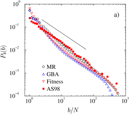
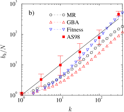
Figure 9: a) Integrated betweenness distribution for the MR, GBA, and fitness models, compared with the result from the AS98 map. The full line on to has slope $-1.1$, corresponding to the Internet map. b) Betweenness $b_{k}$ as a function of the node’s connectivity $k$ corresponding to the previous results. The full line has slope $1.0$.

In Table 4 we report the average values of the connectivity, clustering coefficient, chemical distance, and betweenness for the three models, compared with the respective values computed for Internet during 1998. From the examination of this Table, one could surprisingly conclude that the MR model, which neglects by constructions any correlation among nodes, yields the average values in better agreement with the Internet data. As we can observe, the fitness model provides a too small value for the average clustering coefficient, while the GBA model clearly fails for the average chemical distance and the betweenness. A more crucial test about the models is however provided by the analysis of the full distribution of the various quantities, that should reproduce the scale-free features of the real Internet.

The betweenness distribution $p_{b}(b)$ of the three models give qualitatively similar results. The integrated betweenness distribution $P_{b}(b)$ obtained is plotted in Fig. 9(a). Both the MR and the fitness models follow a power-law decay $P_{b}(b)\sim b^{-\delta}$ with an exponent $\delta\simeq 2$, in agreement with the value obtained from the AS maps. The GBA model shows an appreciable bending which, nevertheless, is compatible with the experimental Internet behavior. These results are in agreement with the numerical prediction in Ref. Goh et al. (2001) and support the conjecture that the exponent $\delta\simeq 2.2$ is a universal quantity in all scale-free networks with $2<\gamma<3$. In order to further inspect the betweenness properties, we plot in Fig. 9(b) the average betweenness $b_{k}$ as a function of the connectivity. In this case, the MR and GBA models yield an exponent $\beta\simeq 1$, compatible with the AS maps, while the fitness model exhibits a somewhat larger exponent, close to $1.4$. Also in this case, we have that the finite size logarithmic corrections present in the fitness model could play a determinant role in this discrepancy.

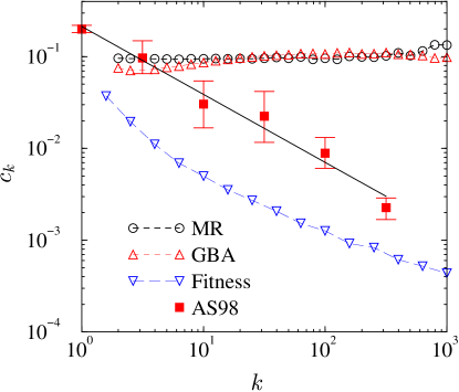
Figure 10: Clustering coefficient $c_{k}$ as a function of the connectivity $k$ for the MR, GBA, and fitness models, compared with the result from the AS98 map. The full line has slope $-0.75$.

Figure 11: Average connectivity of the nearest neighbors of a node as a function of the connectivity $k$ for the MR, GBA, and fitness models, compared with the result from the AS98 map. The AS98 data have been binned for the sake of clarity. The full line has a slope $-0.5$.

While properties related to the betweenness do not appear to pinpoint a major difference among the models, the most striking test is provided by analyzing the correlation properties of the models. In Figs. 10 and 11, we report the average clustering coefficient as a function of the connectivity, $c_{k}$, and the average connectivity of the neighbors, $\left<k_{nn}\right>$, respectively. The data from Internet maps show a nontrivial $k$ structure that, as discussed in previous Sections, is due to scale-free correlation properties among nodes. These properties depend on their turn upon the underlying hierarchy of the Internet structure. The only model that renders results in qualitative agreement with the Internet maps is the fitness model. On the contrary, the MR and GBA models completely fail, producing quantities which are almost independent on $k$. The reason of this striking difference can be traced back to the lack of correlations among nodes, which in the MR model is imposed by construction (the model is a random network with fixed connectivity distribution), and in the GBA model it is due to the destruction of correlations by the random rewiring mechanism implemented. The general analytic study of connectivity correlations in growing networks models can be found in Ref. Krapivsky and Redner (2001), and it is worth noticing that a $k$-structure in correlation functions, as probed by the quantity $\left<k_{nn}\right>$, does not arise in all growing network models. In this perspective we can use correlation properties as one of the discriminating feature among various models that show the same scale-free connectivity exponent.

The fitness model is able to reproduce the non trivial correlation properties because of the fitness parameter of each node that mimics the different hierarchical, economical, and geographical constraints of the Internet growth. Since the model is embedding many features in one single parameter, we have to consider it just as a very first step towards a more realistic modeling of the Internet. In this perspective, models in which the attachment rate depends on both the connectivity and the real space distance between two nodes has been studied in Medina et al. (2000); Yook et al. (2001). These models seem to give a better description of the Internet topology. In particular, the model of Ref. Yook et al. (2001), includes geographical constraints, obtaining that, on average, the probability to connect to a given node scales linearly with its connectivity and it is inversely proportional to the distance to that node. A comparison with real data is, in this case, more difficult because Internet maps generally lack geographical and economical information.

VIII Summary and conclusions

In summary, we have shown that the Internet maps exhibit a stationary scale-free topology, characterized by non-trivial connectivity correlations. An investigation of the Internet dynamics confirms the presence of a preferential attachment behaving linearly with the nodes’ connectivity and identifies two different dynamical regimes during the nodes’ evolution. We have compared several models of scale-free networks to the experimental data obtained from the AS maps. While all the models seem to capture the scale-free connectivity distribution, correlation and clustering properties are captured only in models that take into account several other ingredients, such as the nodes’ hierarchy, resource constraints and geographical location. Other ingredients that should be included in the Internet modeling concern the possibility of including the wiring among existing nodes and age effects that our analysis show to be an appreciable feature of the Internet evolution. The results presented in this work show that the understanding and modeling of Internet is an interesting and stimulating problem that need the cooperative efforts of data analysis and theoretical modeling.