Zone Edge Softening and Relaxation in the Double Exchange Model.

Abstract

The $J\to\infty$ double exchange model is formulated in terms of three auxiliary particles. A slow true bosonic magnon propagates by admixture with a fast fermionic pseudo-magnon. This process involves the absorption of a conduction electron which, for this half-metal, carries only charge degrees of freedom. The magnon dispersion becomes much weaker and the relaxation rate increases rapidly upon approaching the zone boundary. That the magnons relax for all wave vector values implies the existence of a low energy spin continuum.

The double exchange model has a long history. It was introduced by Zener1 fifty years ago in order to explain the phase diagram of La_1-xCa_xMnO₃. With the explosion of interest in the colossal magnetoresistance effect in a number of manganite systems this has again become a model of prime importance. The Hamiltonian is,

$${\cal H}=-J\sum_{i}\vec{S}_{i}\cdot\vec{s}_{i}-\sum_{\sigma nn^{\prime}}t_{nn^{\prime}}(c^{\dagger}_{n\sigma}c_{n^{\prime}\sigma}+H.c.).$$ (1)

Here $J$ reflects the Hund’s rule coupling energy and is taken to be positive and large, i.e., $J>t$. In a seminal paper, de Gennes2 ; 3 showed for near neighbor $t_{nn^{\prime}}$ couplings that in the classical, i.e.,large spin $S$, limit this model has magnon like excitations $\propto(xt/S)(1-\cos q)$, i.e., the dispersion relationship is that of a Heisenberg model. For such large values of $J$ the model is a half-metal. The Fermi level is in the majority band and Stoner excitations have large energies $\sim J$ and are well above the much lower energy magnons.

The experimental situation has been discussed recentlyDai by Dai et al. Materials with high Curie temperatures do have Heisenberg like dispersion relationships but for similar compounds with smaller such temperatures there is a marked softening of the magnons upon approaching the zone boundary. The relaxation rate is also anomalous. The magnon width is quite small for small $\vec{q}$ increasing very strongly for $q$ larger than some critical value. Since this behavior is not explained by double exchange model using the standard theory based upon the large $S$ approach nor by the theory of magnon-magnon interactions, these authors suggest that the coupling to phonon modes is important. The theoretical understanding has been summarizedKK by Khaliullin and Kilian. They also emphasize that the experimental situation cannot be explained by the usual theory and develop a large $S$ approach which includes coupling to Jahn-Teller phonons and which can explain experiment.

In this Letter will be presented a novel analytic theory of the basic $\cal H$, Eqn. (1), which shows that the two experimental effects attributed to phonons do in fact occur within the simple double exchange model. This new approach is based upon the auxiliary particle method. There are three such particles, a $b$-boson which reflects the true, slow, magnons, the $c$-fermion which represents the charge degrees of freedom of the conduction electrons and a $t$-fermion which corresponds to a spin deviation at a site with a charge carrier.

In fact, the earlier exact diagonalization studies of Zang et al., 4 and Kaplan and Mahanti 5 for the one dimensional model indicate the existence of zone boundary softening. In particular for $S=1/2$ and small concentrations the magnon dispersion deviates strongly from $(1-\cos q)$. Very recently Kaplan et al., 7 have performed new exact diagonalization studies again for one dimension and in the limit $J\to\infty$. Contrary to popular belief and mean field theory, they find spin excitations with energies much less that $J$. These they associate with a non-Stoner continuum and speculate that this continuum comes down to zero energy in the thermodynamic limit. In contrast, Golosov 8 using the large $S$ expansion up to fourth order claims that magnon-electron scattering does not give rise to magnon damping this implying that the magnons do not enter a continuum at low energies.

Mathematically the present approach is based upon an expansion in $x$ the concentration of carriers. For small $x$, $S=\frac{1}{2}$ and one dimension our results for the magnon dispersion agree well with those of exact diagonalization. Useful results are obtained for $x$ as large as $3/16$ even for $S=1/2$. The magnons can exchange energy and momentum which the charge excitations and all finite $\vec{q}$ excitations have a non-zero relaxation rate confirming the existence a low energy non-Stoner continuum. For $q<k_{F}$, the Fermi wave vector, relaxation is reduced by phase space considerations. A rapid onset of relaxation will therefore occur around $q\approx k_{F}$. Although most of the results presented here are for one dimension, these principal conclusions are also valid for higher dimensions and some such results will be given. The present approach does not include orbital degeneracy nor phonons and the authors recognize that these are important physical ingredients for real materials. The method is easily generalized to include such effects and might form the basis for a comprehensive theory at least for modest $x$ values.

Consider a single spin deviation relative to the ferromagnetic ground state for an odd number of electrons. In the $J\to\infty$ limit, for a given site $n$, there are only four states of interest. There is the state $\left|S,0\right\rangle$ with $S_{z}=S$ and no electron and which is considered to be the “vacuum”. The state $\left|S-1,0\right\rangle$ has the spin deviated and is mapped to a state $d^{\dagger}_{n}|\rangle$ which has a $d$-boson created on this vacuum. An un-deviated state with an up conduction electron is $\left|S,\uparrow\right\rangle$ and maps to the $c$-fermion state $c^{\dagger}_{n}|\rangle$. Lastly, a state which has a total spin $S+\frac{1}{2}$ but $S_{z}=S-\frac{1}{2}$ is $\frac{1}{\sqrt{2S+1}}\left[\sqrt{2S}\left|S-1.\uparrow\right\rangle+\left|S,\downarrow\right\rangle\right]$ with $t^{\dagger}_{n}|\rangle$ as its map. The particles are “hard core”, i.e., the total number $Q_{n}=n^{c}_{n}+n^{d}_{n}+n^{t}_{n}\leq 1$, where, e.g., $n^{t}_{n}=t^{\dagger}_{n}t_{n}$. The total number of conduction electrons $\hat{N}=\sum_{n}\left(n_{n}^{c}+n_{n}^{t}\right)$ does not involve $d^{\dagger}_{n}$.

Subject to $Q_{n}\leq 1$ the low energy part of the Hamiltonian maps exactly to,

$${\cal H}=-\sum_{nn^{\prime}}t_{nn^{\prime}}(\tilde{c}^{\dagger}_{n^{\prime}}\tilde{c}_{n}+\frac{1}{2S+1}\tilde{t}^{\dagger}_{n^{\prime}}\tilde{t}_{n}+H.c.)$$ (2)

$$+ \sqrt{\frac{2S}{2S+1}}\sum_{nn^{\prime}}t_{nn^{\prime}}(t^{\dagger}_{n^{\prime}}d_{n^{\prime}}c_{n}+c^{\dagger}_{n^{\prime}}d^{\dagger}_{n}t_{n}+H.c.).$$

where, e.g., $\tilde{c}_{n}=c_{n}(1-n^{t}_{n}-n^{d}_{n})$. When ${\cal H}$ acts on a state which satisfies $Q_{n}\leq 1$, the result is also consistent with this constraint, i.e., this representation of the Hamiltonian does not mix physical with unphysical states.

The Hamiltonian is written as ${\cal H}^{\prime}-\mu\hat{N}+I_{c}$ where $I_{c}=t\sum_{n}[(\tilde{c}^{\dagger}_{n^{\prime}}\tilde{c}_{n}-c^{\dagger}_{n+1}c_{n})+(1/(2S+1))(\tilde{t}^{\dagger}_{n+1}\tilde{t}_{n}-t^{\dagger}_{n+1}t_{n})+H.c.]$ comprises the operators which enforce the constraint. Then the Fourier transform of,

$${\cal H}^{\prime}-\mu\hat{N} =$$

$$\sum_{\vec{k}}(\epsilon_{\vec{k}} - \mu)c^{\dagger}_{\vec{k}}c_{\vec{k}}+\frac{1}{2S+1}\sum_{\vec{k}}\left(\epsilon_{\vec{k}}-\mu\right)t^{\dagger}_{k}t_{k}$$

$$-\sqrt{\frac{2S}{2S+1}} \hskip-20.0pt\frac{1}{N}\sum_{k,q}\epsilon_{\vec{q}}(t^{\dagger}_{\vec{k}+\vec{q}}d_{\vec{k}}c_{\vec{q}}+c^{\dagger}_{\vec{q}}d^{\dagger}_{\vec{k}}t_{\vec{k}+\vec{q}}+H.c.),$$ (3)

where $\epsilon_{\vec{k}}=-\sum_{j}t_{ij}e^{i\vec{k}\cdot(\vec{r}_{j}-\vec{r}_{j})}$. The most important part of $I_{c}$ is,

$$\frac{1}{N^{2}}\sum_{\vec{k}\vec{k}^{\prime},\vec{q}}\epsilon_{\vec{q}}\left(c^{\dagger}_{\vec{k}+\vec{q}}c_{\vec{k}}d^{\dagger}_{\vec{k}^{\prime}-\vec{q}}d_{\vec{k}^{\prime}}\right)+H.c.,$$ (4)

since this leads to the renormalization of the conduction electron wave function near the deviated spin. In the magnon dispersion relationship, the leading term O($x,t$) is an unimportant constant. The O($x,t^{2}$) term produces renormalization and relaxation and will be discussed below.

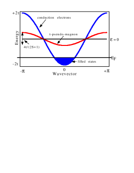
Figure 1: For one dimension, the conduction electron, or $c$-particle, band has width $D=4t$ while the pseudo-magnon, i.e., $t$-fermion, band is a factor of $2S+1$ narrower

In the zeroth order approximation, for small $x$, the conduction electrons occupy the region near $k=0$ at the bottom of a band of total width $D$. The $t$-particle band has a smaller width $[D/(2S+1)]$ and for small $x$ this band will not have a real occupation, see Fig. 1. The deviated spin, associated with the $d$-particle, has no zero order dispersion. This becomes dispersive by admixture into the $t$-particle. There are matrix elements, $\sqrt{2S}$, of the total spin which connect the vacuum with the boson $d^{\dagger}_{k}$, i.e., this is a true magnon. There are also matrix elements, $\sqrt{2S+1}$, which connect $c_{k}$ with $t^{\dagger}_{k+q}$, so the finite wave-vector total spin operator,

$$S^{+}_{\vec{q}}=\sqrt{2S}d^{\dagger}_{\vec{q}}+\sqrt{2S+1}\sum_{\vec{k}}(t^{\dagger}_{\vec{k}+\vec{q}}c_{\vec{k}}+H.c.).$$ (5)

For small $x$ the dispersion in energy and momentum of the conduction electron, $c$-particles, is relatively small and so, for the second term, the $t$-fermion dominates the $q$ dispersion. Since it has a band width $\sim D/S$ the $t$-fermion can be identified as the fast pseudo-magnon with a large gap $\sim D/2$.

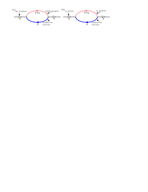
Figure 2: (a) A true, $d$-particle, magnon decays into a pseudo-magnon, i.e., a $t$-particle, upon absorbing a conduction electron $c$-particle. The momentum is conserved and each vertex is $\sqrt{2S/(2S+1)}(\epsilon_{\vec{q}}/N)$. This leads to Eqn. (6). (b) The equivalent for the ferromagnetic state. The $b_{0}$-boson, which reflects the state $|S,0\rangle$, decays to a $f_{0}$-fermion, which corresponds to $|S,\uparrow\rangle$, upon absorbing a conduction electron. This is reflected by Eqn. (8).

The leading approximation for the dispersion of the slow magnon, corresponds to the Feynman diagram shown in Fig. 2a,

$$\omega_{\vec{q}}=\frac{2S}{2S+1}\frac{1}{N}\sum_{\vec{k}}{\epsilon_{\vec{k}}}^{2}\frac{n_{\vec{k}}}{\epsilon_{\vec{k}}-\frac{1}{2S+1}\epsilon_{\vec{k}+\vec{q}}}$$ (6)

where $n_{\vec{k}}$ is the usual conduction electron thermal occupation factor. Since it involves a single sum over the occupied conduction electron states $\omega_{\vec{q}}\sim x$ which shows that the $d$-true-magnon moves slowly for small $x$.

It is important to confirm that the present method does not give a false spin gap. In order to compare like with like, the problem with no reversed spins is formulated using a method in which a single site is treated specially so that the same approximation as used above for the deviated $d$-particle site, can be made for this special site. There are two, rather than a single operator for this “impurity” site, taken to be at the origin,. The absence of a particle corresponds to an unphysical vacuum $|\rangle_{0}$. The maximum spin state without a conduction electron, $|S,0\rangle$, is mapped to $b^{\dagger}_{0}|\rangle_{0}$ while $|S,\uparrow\rangle$, when a conduction electron is present, is reflected by $f^{\dagger}_{0}|\rangle_{0}$. The manifold with no reversed spins then corresponds to,

$${\cal H}-\mu\hat{N}=-\sum_{nn^{\prime}}t_{nn^{\prime}}(\tilde{c}^{\dagger}_{n}\tilde{c}_{n^{\prime}}+H.c.)-\mu\sum_{n\neq 0}c^{\dagger}_{n}c_{n}$$ (7)

$$+ \sum_{n\neq 0}t_{0n}\left[(f^{\dagger}_{0}b_{0}(c_{n}+c_{N-n+1})+H.c.\right]-\mu f^{\dagger}_{0}f_{0}.$$

With this unusual representation of the ferromagnetic ground state it is possible to make the same approximations as with a single deviation and a self-energy, Fig. 2b, for the $b$-particle, the equivalent to the $d$-particle. This gives for the energy,

$$\omega_{0}=\frac{1}{N}\sum_{k}{\epsilon_{\vec{k}}}^{2}\frac{n_{\vec{k}}}{\epsilon_{\vec{k}}}=\frac{1}{N}\sum_{k}\epsilon_{\vec{k}}n_{\vec{k}},$$ (8)

which, surprisingly, is the exact answer. Clearly Eqn. (8) agrees with Eqn. (6) when $\vec{q}=0$ which indeed confirms that there is no gap in the magnon spectrum.

It should also be that $\omega_{\vec{q}}$ agrees with the (corrected) result of de Gennes for large enough $S$. The large $S$ expansion for the one dimensional near neighbor model, i.e., with $\epsilon_{\vec{k}}\to-2t\cos k$ gives,

$$\omega_{q}-\omega_{q=0}=\frac{1}{2S}\left[\frac{1}{N}\sum_{k}2t\cos kn_{k}\right](1-\cos q)$$ (9)

which agrees with Furukawa3 .

It is also possible to obtain an analytic result for small enough $x$ independent of $S$. Assuming that the conduction electron Fermi surface contracts to a point, gives,

$$\omega_{q}-\omega_{q=0}\approx\frac{4xtS}{2S+1}\frac{1}{1-\frac{\cos q}{2S+1}}.$$ (10)

For small values of $S$, this expression gives a dispersion which becomes rather flat near the zone edges, see below.

It is the slow $d$-magnon which is to be identified with the low energy magnon branch found in the numerical work 4 ; 5 ; 7 . In Fig. 3 are compared the numerical results 4 for $S=1/2$ with the present Eqn. (6). For $x=1/16$ and $3/16$ the flattening of the dispersion near the zone edge seen in the numerical data is well reproduced although the difference between the two different concentrations is not as great as in the numerical data. For $S=1/2$ and $x=5/16$ the Fermi surface lies in the $t$-particle band and the assumptions used for Eqn. (6) are not valid. The result Eqn. (6) and the small $x$ and the large $S$ approximations are compared, for $S=1/2$, in Fig. 4. The small $x$ approximation compares well with $x=1/16$ even for $S=1/2$. In contrast the agreement with the large $S$, simple $\cos k$, result is not at all good. The deviations from a simple cosine are therefore well reproduced by Eqn. (10) and are clearly most extreme for $S=1/2$.

As the small $x$ approximation illustrates, the fattening near the zone edges occurs because, for small $S$, the dispersion of the virtual $t$-particle is comparable with its energy.

Since the effective exchange increases with increasing $x$ so will the Curie temperature, $T_{c}$. Larger $x$ values, Fig. 3, have a dispersion which approaches that of a Heisenberg model. It follows for larger $x$ and $T_{c}$ values, the small $\vec{q}$ magnon stiffness will accord with $T_{c}$. It is a commonplace observation that the zone edge softening which occurs for smaller $x$ values will cause $T_{c}$ to fall short of that predicted by this initial stiffness. This appears to be the case experimentallyDai .

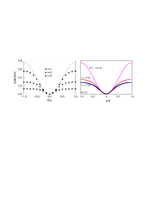
Figure 3: The right box corresponds to the present theory for concentrations $x=1/16$ and $x=3/16$ for spin $S=1/2$. The top curve corresponds to $A(1-\cos q)$. The scales where chosen so that all curves coincide at $q=0.125\pi$. The small $x$ result Eqn. (10) cannot be distinguished from the result for $x=1/16$. The left box shows the numerical results 4 with $n$ electrons and 16 sites. Again the scales cause the points at $q=0.125\pi$ to coincide with each other and the $A(1-\cos q)$ solid line.

It is evident from the Hamiltonian, in the form Eqn. (3), that there is a continuum of low energy longitudinal, i.e., charge excitations of the conduction electron $c$-particles. The question is whether the spin excitations couple to the continuum of charge excitations. This is the case and such a coupling shows up as a finite relaxation rate for the $d$-magnons. In one dimension the leading order relaxation process for this slow magnon has an onset for relaxation which occurs only at finite momentum indicating that this low energy branch enters a continuum for finite momentum. This relaxation corresponds to the Feynman diagrams shown in Fig. 5. Corresponding to Fig. 5a is a second order process which involves $I_{c}$, while Fig. 5b is of fourth order and uses the vector $t$-fermion in the extra intermediate states. There is also interference between the two processes. The net relaxation rate is of the form:

$$\approx \pi\frac{{t^{\prime}}^{2}}{N^{2}}\sum_{p^{\prime},q}n_{q}(1-n_{p+q-p})$$

$$\times\delta(\omega_{q} + 2t\cos k-(\omega_{p}+2t\cos(q+k-p)),$$ (11)

where $t^{\prime}\approx t+[2S/(2S+1)](2t^{2}/|\mu|)$.

A particle-hole charge excitation of the conduction electron is created and takes away energy and momentum from the magnon. Since only the initial state electron lies below the Fermi surface, such a process is proportional to $x$. The only energy scale is $t$ (e.g.,$|\mu|\sim t$) but relaxation is strongly suppressed due to phase space considerations. In order to understand the trends, consider small $x$ and larger values of $S$. This implies that the energy dispersion of the magnon is negligible as compared to that of the conduction electrons. It is not possible to conserve both energy and momentum for small values of the magnon $q$ since the energy of the conduction electron charge excitations with the same momentum is too large. Small energy but large $q$ particle-hole excitations imply that the electrons scatter from $\mp k_{F}\to\pm k_{F}$ and have a momentum transfer of $\approx 2k_{F}$. In order to minimize the initial magnon momentum it must scatter from $\mp k_{F}\to\pm k_{F}$, i.e., the onset of magnon relaxation will occur for $q\approx\pm k_{F}$ a momentum which is proportional to $x$ for one dimension. The finite magnon dispersion implied by smaller values of $S$ and larger $x$ will reduce this threshold value of $q$ from this limiting value of $\pm k_{F}$.

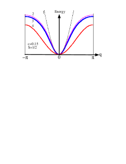
Figure 4: Curve “3” is Eqn. (6), with $x=0.15$, for $\omega_{q}$ and is almost indistinguishable from curve “2” which reflects the approximation $\frac{4xtS}{2S+1}\frac{1}{1-\frac{\cos q}{2S+1}}-2xt$. Curve “4” is the large $S$ approximation $4xt[S/(S+1)^{2}](1-\cos q)$ while curve “1” is similar but made to fit the $q^{2}$ dependence of “3” for small $q$.

However higher order processes have a final state which still comprises a single magnon but now reflects a pair of conduction electron particle-hole excitations. Even with an arbitrary small initial magnon momentum it is always possible to find a pair of particle hole excitations which, e.g., go from close to one Fermi surface to the other ($\pm k_{F}\to\mp k_{F}$) but in opposite senses and which have any small energy and moment. Thus as $x$ increases the pseudo-gap to momentum $\approx\pm k_{F}$ progressively fills.

!

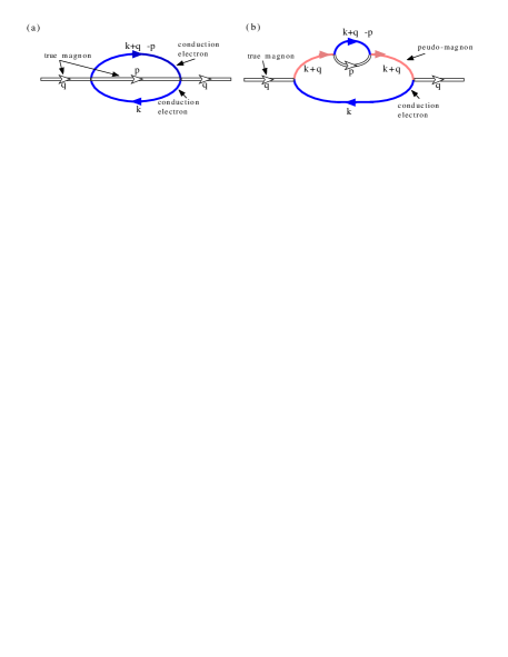
Figure 5: (a) A momentum $q$ magnon relaxes via $I_{c}$ to momentum $p$ transferring energy and momentum to a particle-hole conduction electron pair. (b) The same process but using the $t$-fermion as intermediate particle.

Much of the above discussion generalizes to two and three dimensions. In particular the small $x$ approximation,

$$\omega_{\vec{q}}=\frac{2x\epsilon_{\vec{k}=0}S}{2S+1}\frac{1}{N}\frac{1}{1-\frac{1}{2S+1}(\epsilon_{\vec{q}}/\epsilon_{\vec{k}=0})}$$ (12)

exhibits softening at the zone edges and relaxation will be phase space limited for $q<k_{F}$ even though there is no longer a threshold for the second order process. Evidently the orbital degeneracy of the real materials is of great importance. This will be dealt with elsewhere.

This work was supported by a Grant-in-Aid for Scientific Research on Priority Areas from the Ministry of Education, Science, Culture and Technology of Japan, CREST. SEB is on sabbatical leave from the Physics Department, University of Miami, Florida, USA and wishes to thank the members of IMR for their kind hospitality. SM acknowledges support of the Humboldt Foundation.

References

- (1) C. Zener, Phys. Rev. 82, 403 (1951).
- (2) P. G deGennes, Phys. Rev. 118, 141 (1960).
- (3) See: N. Furukawa, J. Phys. Soc. Jpn. 64, 3164 (1995); 65, 1174 (1996); 68, 2522 (1999).
- (4) P. Dai et al., Phys. Rev. B61, 9553 (2000).
- (5) G. Khaliullin and R. Kilian, Phys. Rev. B61, 3494 (2000).
- (6) Jun Zang, H. Röder, A. R. Bishop and S. A. Trugman J. Phys.: Condens. Matter 9, L157 (1997)
- (7) T. A. Kaplan and S. D. Mahanti, J. Phys. Condens. Matter 9, L291 (1997).
- (8) T. A. Kaplan, S. D. Mahanti and Y.-S. Yu, Phys. Rev. Letts. 86, 3634 (2001).
- (9) D. I. Golosov, Phys. Rev. Letts. 84, 3974 (2000).