Abstract

We study the universality class of the fixed points of the 2D random bond $q$-state Potts model by means of numerical transfer matrix methods. In particular, we determine the critical exponents associated with the fixed point on the Nishimori line. Precise measurements show that the universality class of this fixed point is inconsistent with percolation on Potts clusters for $q=2$, corresponding to the Ising model, and $q=3$.

Nishimori point in random-bond Ising and Potts models in 2D

Introduction

During the last decade, the study of disordered systems has attracted much interest. This is true in particular in two dimensions, where the possible types of critical behavior for the corresponding pure models can be classified using conformal field theory [1]. Recently, similar classification issues for disordered models have been addressed through the study of random matrix ensembles [2], but many fundamental questions remain open.

An important category of 2D disordered systems is given by models where the disorder couples to the local energy density (random Potts models). Here we shall study such models that interpolate between ferromagnetic random bond disorder, and a stronger $\pm J$ type disorder. Our main focus shall be on the cases with $q=2$ (Ising) or $q=3$ states.

1 Phase Diagram

The Ising model on a square lattice is one of the most popular two-dimensional systems. It is specified by the energy of a spin configuration

$${\cal H}(\{S_{i}\})=\sum_{\langle i,j\rangle}J_{ij}\delta_{S_{i},S_{j}}\,,$$ (1)

where the sum is over all bonds and the coupling constants $J_{ij}$ are bond dependent. Different distributions of disorder can be considered. The most common ones are the $J_{ij}=\pm 1$ and the Gaussian distribution of disorder. In this work we will study in particular the $J_{ij}=\pm 1$ Random-Bond Ising Model (RBIM) with the following probability distribution:

$$P(J_{ij})=p\delta(J_{ij}-1)+(1-p)\delta(J_{ij}+1)\,.$$ (2)

The topology of the phase diagram of the RBIM depends crucially on the type of disorder one considers. An instructive example is provided by a disorder having only two possible values for the bonds with equal signs and probabilities. It is by now well established [3] that the only non-trivial fixed points are located at the extrema of the boundary of the ferromagnetic phase, corresponding to the pure Ising fixed point and a zero temperature fixed point which turns out to be in the percolation universality class.

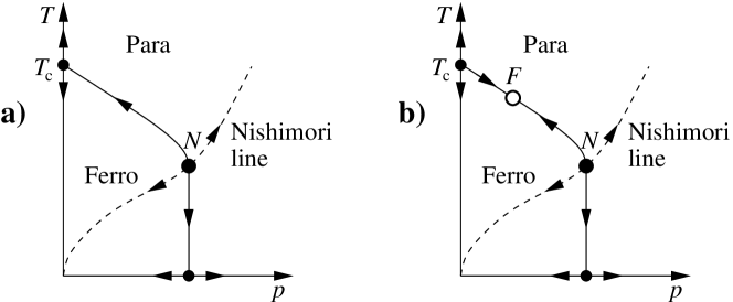
Figure 1: Phase diagram of the two-dimensional $\pm J$ random-bond Ising (a) and $q>2$ Potts (b) models. Note the additional ferromagnetic fixed point F in the Potts model (b).

When the distribution contains also bonds with different signs (like in (2)), the situation is more subtle. In particular, it is known since the work of McMillan [4] that there exists an unstable fixed point at finite temperature and a finite value of disorder $p_{c}$ and another fixed point at zero temperature and a value of disorder $p\simeq p_{c}$ (McMillan obtained these results with a Gaussian distribution of disorder). Thus for the RBIM, one expects three fixed points (see Fig. 1a): i) the fixed point corresponding to the case without disorder. Close to this point, one expects that the physics is just described by the usual perturbation of the Ising model with weak disorder [5, 6, 7, 8], i.e. one flows back to the model without disorder. ii) A random fixed point $N$ at finite temperature and a finite value of disorder. Describing this unstable fixed point is the main purpose of this work. Since this fixed point is unstable under two parameters (temperature and disorder) it is very difficult to study numerically. We will come back to this point later. iii) Finally, there is a third fixed point at zero temperature but non-vanishing disorder. The universality class of this last fixed point is also unknown at present.

For the more general case of the random $q$-state Potts model (RBPM) with $q>2$, the situation is slightly more complicated. We define this model by

$${\cal H}(\{S_{i}\})=-\sum_{\langle i,j\rangle}\delta^{(q)}(S_{i}-S_{j}+J_{ij})\,,$$ (3)

where $S_{i}=1,2,\ldots,q$, and $\delta^{(q)}(x)=1$ if $x=0\mbox{ mod }q$ and zero otherwise. The randomness now takes the form of a local “twist” $J_{ij}$, which is clearly a more severe type of disorder than simple bond randomness. The variables $J_{ij}$ are taken from the distribution

$$P(J_{ij})=\big{(}1-(q-1)p\big{)}\delta(J_{ij})+p\sum_{J=1}^{q-1}\delta(J_{ij}-J)\,,$$ (4)

with $0\leq p\leq 1/(q-1)$ controlling the strength of the randomness. We shall refer to this model, which was originally introduced in Ref. [9], as the Potts Gauge Glass (PGG). The particular form of the randomness ensures the existence of a Nishimori line (see below). For $q=2$, the PGG reduces to the RBIM, and for $p=1/q$ it was studied analytically in [10]. The PGG is also connected to the RBPM: When $q>2$ the pure Potts model ($p=0$) should be unstable to a small amount of randomness, meaning that the renormalization group (RG) flow cannot be as indicated in Fig. 1a. Indeed, the existence of a new fixed point F between the pure and random fixed points (see open circle in Fig. 1b) is now well established analytically [8, 11] and numerically for $q=3$ [12]. If $(q-2)$, and hence the value of $p$ at F, is sufficiently small, frustration effects are negligible, and we should flow to the same random fixed point for any kind of randomness. For reasons of continuity we expect this argument to hold true also for higher values of $q$ [3].

As mentioned above, a numerical study of the random fixed point $N$ at finite temperature and finite disorder is a difficult task since it is unstable in both of its parameters. Fortunately, for a certain class of probability distributions, Nishimori has shown that a so-called ‘Nishimori’ line exists where many properties can be calculated exactly [13]. For the RBIM with the probability distribution (2), this line is given by

$${\rm e}^{\beta}={1-p\over p}\,,$$ (5)

with $\beta=1/T$. On the Nishimori line, the internal energy can be calculated exactly and an upper bound can be given for the specific heat. Also of interest is an equality of the moments of the spin correlation functions (see below). Nishimori has further proved inequalities for the correlation functions which yield important constraints on the topology of the phase diagram which is shown in Fig. 1a for the $\pm J$ RBIM. Since the Nishimori line is also invariant under Renormalization Group (RG) transformations [14], the intersection of the Nishimori line and the Ferro-Para transition line must be a fixed point which is identified with the random fixed point $N$. This so-called Nishimori point corresponds to a new universality class. The full line in the phase diagram Fig. 1a is the phase boundary between the ferromagnetic and paramagnetic regions. In two dimensions and at zero temperature, the RBIM has a phase with spin glass correlations [15]. The three non-trivial fixed points along the full line are the pure Ising fixed point, the Nishimori point N at the crossing with the Nishimori line (dotted line) and the zero temperature point whose properties are still mostly unknown.

For the $q$-state random Potts model with $q>2$, a Nishimori line can also be obtained [9]. Reexpressing the disorder distribution as

$$P(J_{ij})=pe^{K\delta^{(q)}(J_{ij})}\;\;\hbox{with}\;\;K=\log\big{(}1/p-(q-1)\big{)}$$ (6)

the Nishimori line is given by the condition $K=\beta$ which generalizes (5) to $q>2$. We refer to [16] for more details.

Note that the existence of a random fixed point is not related to the existence of a Nishimori line. One could have chosen a distribution of disorder for which no Nishimori line exist, still a random fixed point would exist. This was observed for instance by Sørensen et al. [12] for the $q=3$ random bond Potts model with a distribution of disorder different from (4). The main advantage of the Nishimori line is that it allows to locate the random fixed point while scanning only one parameter.

Over the last years, many numerical and analytical efforts have been made in order to identify the universality class of the Nishimori point. There is a long list of numerical results [4, 17, 18, 19, 20, 21] with values for the critical exponents that are very close to those of percolation

2 Results

We now turn to our numerical results. These were obtained by extensive numerical transfer-matrix calculations of the Nishimori point with the binary bond distribution (2) for $q=2$ and with the distribution (4) for $q=3$ on the square lattice.

The first set of results is based on measurements of the effective central charge, which is a very efficient way to locate a fixed point. The effective central charge $c$ is obtained as the universal coefficient of the finite-size correction to the free energy per site for periodic boundary conditions [22]

$$f_{L}^{(p)}=f_{\infty}^{(p)}+{c\pi\over 6L^{2}}+\cdots.$$ (7)

We first turn our attention to the determination of the properties of the weak random point for $q=3$. The finite-size estimates for the effective central charge increase along the massless RG flows and approach the fixed point values for $L\to\infty$. Note that this does not contradict Zamolodchikov’s $c$-theorem [23] since the present theories are not unitary. The Ferro-Para boundary (cf. Fig. 1b) can be traced by identifying the maximum of the finite-size estimates of $c$ as a function of $T$, for various fixed values of $p$.

Since the randomness is strong, and since the fits to (7) must be based on at least two different sizes $L$ to eliminate the non-universal quantity $f_{\infty}^{(p)}$, we have taken several precautions [16] in order to obtain small error bars on the $f_{L}^{(p)}$. Our strips have length $N=10^{5}$, and we average $f_{L}^{(p)}$ over up to $10^{5}$ independent realizations.

The measurement of the effective central charge at the Ferro-Para boundary as a function of $p$ shows the existence of an attractive fixed point at $p\sim 0.04$ with a central charge slightly larger than $c_{\rm pure}=4/5$, characterizing the pure 3-state Potts model. After extrapolation [16], we arrive at the final result

$$c_{F}=0.8025(10)\,,$$ (8)

which compares favorably with the perturbative result $c_{\rm pert}=0.8026+{\cal O}\left((q-2)^{5}\right)$ [8, 11] for the $q=3$ RBPM.

The next result is the numerical location of the Nishimori point along the Nishimori line [24]. Again, this can be done by measuring $c$ along the Nishimori line. For the $q=2$ case, we have used the domain-wall free energy [4] to locate the critical concentration of disorder $p_{c}$ since it provides a better precision. For a strip of width $L$ the domain-wall free energy $d_{L}$ is defined as (omitting a factor of $\beta$)

$$d_{L}=L^{2}\left(f_{L}^{(p)}-f_{L}^{(a)}\right)\,,$$ (9)

where $f_{L}^{(p)}$ is the free energy per site of a strip of width $L$ with periodic boundary conditions and $f_{L}^{(a)}$ the corresponding one with antiperiodic boundary conditions. $d_{L}$ is an observable which can be used directly to study the RG flow under scale transformations. In particular, it is constant at a fixed point.

We have computed $f_{L}^{(p)}={\ln Z^{(p)}\over LN}$ and $f_{L}^{(a)}={\ln Z^{(a)}\over LN}$ employing a standard transfer matrix technique with sparse matrix factorization (see, e.g., [25]) on strips of length $N=10^{6}$. Again, special tricks are used to reduce fluctuations [24]. We used around 1000 to 4000 samples of $L\times 10^{6}$ strips to obtain sufficiently small error bars for $L\leq 12$.

Figure 2: Domain-wall free energy for $q=2$ along the Nishimori line (5). The inset shows the raw data and the main panel the scaling collapse with $p_{c}=0.1094$ and $\nu=1.33$.

The inset of Fig. 2 shows $d_{L}(p)$ along the Nishimori line (5) in the vicinity of the critical concentration $p_{c}$. A finite-size estimate for $p_{c}$ is given by the crossing points $d_{L_{1}}(p_{c})=d_{L_{2}}(p_{c})$. After extrapolation to an infinitely wide strip, one obtains

$$p_{c}=0.1094(2)\;.$$ (10)

This estimate improves upon the accuracy of earlier estimates [17, 18, 20, 21]. It agrees perfectly with the transfer matrix computations [17, 21], in particular a very recent one [26], while we find a slightly smaller value of $p_{c}$ than [18, 20].

One an also extract the value of $\nu$ from (9). We obtained $\nu\approx 1.33$ [24]. Merz and Chalker [26] were able to go to much larger strip widths and obtained the probably more accurate result $\nu\approx 1.50$. While our estimate was compatible with the value for percolation $\nu=4/3$ [27], the one of [26] is not.

Next, we discuss the effective central charge $c$ for $q=2$. One has $c=1/2$ for the critical point of the pure Ising model, but it has not been determined yet for the Nishimori point. In the process of computing $d_{L}$ we have also obtained estimates of $f_{L}^{(p)}$ for different values of $p$. One can either fit these values for $f_{L}^{(p)}$ exactly by (7) ignoring further corrections in which case the data for the smallest values of $L$ should not be used. Or one includes a correction term of the form $L^{-4}$ which improves the convergence with system size. These two approaches yield consistent estimates for a given $p$. In addition, one can test that the result does not change significantly if other higher-order corrections are added. It should also be noted that the sensitivity of the estimates for $c$ with respect to the location of $p_{c}$ is negligible in comparison with the errors coming from the finite-size analysis. The final result is that the following is a safe estimate for $c$ at the Nishimori point of the $\pm J$ RBIM:

$$c=0.464(4)\,.$$ (11)

This should be compared to the value for percolation over Ising clusters $c={5\sqrt{3}\ln{2}\over 4\pi}\approx 0.4777$ [3]. Even if our result (11) is close to this value, it appears safe to conclude that the Nishimori point is not in the universality class of percolation, at least not the one expected from Ising clusters.

The situation seems rather different for the case $q=3$. In that case, the numerical location of the Nishimori point was only made by measuring $c$ along the Nishimori line and determining the point for which one obtains a maximum. We find [16] a fixed point N at $p_{N}=0.0785(10)$ with a central charge estimate

$$c_{N}=0.756(5)\,.$$ (12)

This is in remarkable agreement with the value of the central charge for the percolation limit in the $q=3$ RBPM: $c=\frac{5\sqrt{3}\ln{3}}{4\pi}\approx 0.7571$ [3]. Below we shall return to the question whether the Nishimori point is “just” percolation. We should also mention that for the case $q=3$ the error bars have been obtained by extrapolating the data assuming that for each fit the relative deviation from the infinite-size result is the same as in the pure model. Taking a more conservative approach as we have done for the case $q=2$ would produce larger error bars, but the conclusion would remain the same.

Another important quantity is the magnetic exponent $\eta$. This exponent can be measured, for example, by computing spin-spin correlation functions. As mentioned earlier, along the Nishimori line the moments of these correlation functions are equal two by two (for $q=2$):

$$[\langle S(x_{1},y_{1})S(x_{2},y_{2})\rangle^{2k-1}]=[\langle S(x_{1},y_{1})S(x_{2},y_{2})\rangle^{2k}]$$ (13)

for any integer $k$. Here $[\cdots]$ stands for the average over the disorder. Assume now that the correlation functions (13) decay algebraically on a plane and define by $x,y$ the coordinates on the infinite cylinder of circumference $L$, with $x\in[1,L]$ and $y\in]-\infty,+\infty[$. Using a conformal mapping, one infers then the following behavior of the correlation functions on the cylinder:

$$[\langle S(x_{1},y)S(x_{2},y)\rangle^{n}]\propto\left(\sin\left({\pi(x_{2}-x_{1})\over L}\right)L\right)^{-\eta_{n}}\,.$$ (14)

For a pure system, one has $\eta_{n}=n\times\eta$. On the other hand, in the case of percolation over Ising clusters, the moments of spin correlation functions are all equal, whence all $\eta_{n}=\eta$ at the critical point.

In order to verify this we have calculated the spin-spin correlation functions on cylinders of width $L$ and length $400\times L$, (i.e. with the length $\gg L$) for $L$ up to 20. We have checked that for width $L=12$, lattice and finite length corrections are of order 1%. One example of these correlation functions can be seen in Fig. 3 (for $q=2$ with $x_{1}=y=0$ and $x_{2}=x$) on a doubly logarithmic scale. One observes that the correlation functions nicely obey the power law (14), thus verifying both the correct location of the critical point as well as the functional form of the spin-spin correlation function in a finite strip.

Figure 3: Moments of the spin-spin correlation function for $q=2$, $p=0.1095$ and $L=20$. We only show the odd moments: $n=1$ ($+$), $n=3$ ($\times$), $n=5$ ($*$) and $n=7$ (open boxes). Error bars are smaller than the size of the symbols. The values of the exponents are given in (15).

We can then fit the exponents by studying the dependence with distance of the correlation functions (14) or by studying the dependence with $L$ for the fixed location $x=L/2$. The first method has proven to give smaller error bars and we obtain for the family of exponents $\eta_{n}$ for $p_{c}=0.1095$ and $L=20$:

$$\eta_{1} = \eta_{2}=0.1854;\qquad\eta_{3}=\eta_{4}=0.2561$$

$$\eta_{5} = \eta_{6}=0.3015;\qquad\eta_{7}=\eta_{8}=0.3354\,,$$ (15)

with relative errors at most of the order of 1%.

One immediately notices two things:

i) The value for $\eta_{1}$ differs considerably from the value of percolation $\eta=5/24\approx 0.2083$ (see, e.g., [27]),

ii) the exponents for higher moments are also considerably different from $\eta_{1}$ which is also clear from inspection of Fig. 3.

We have also calculated estimates for the exponents assuming different values for $p_{c}$, namely, $p_{c}=0.109$ and $0.110$ and the results are still distinct from the ones of percolation (we obtain $\eta_{1}=0.180(1)$ for $p=0.109$ and $\eta_{1}=0.190(1)$ for $p=0.110$). Moreover, it is only in the region very close to $p=0.1095$ that we obtain a stable estimate for $\eta_{1}$ as we increase the width $L$ of the lattices. One can then conclude from the exponents controlling the algebraic decay of the correlation functions that the Nishimori point is not in the percolation universality class.

The same measurements were also performed in the case of $q=3$, for which case the largest system size employed was $L=12$. Performing the same fit of the data, we obtain the following exponents for $p=0.080$

$$\eta_{1} = 0.21239(35);\qquad\eta_{2}=0.25192(39)$$

$$\eta_{3} = 0.30824(47);\qquad\eta_{4}=0.33773(52)\,,$$ (16)

the corresponding values for $p=0.079$ being some 6% smaller.

Although our value of $\eta_{1}$ is now consistent with percolation, this scenario can be excluded by considering the higher moments.

3 Conclusions

In conclusion, we have studied the $\pm J$ random-bond Ising model as well as a $q$-state (Potts-like) generalization that allows for the definition of a Nishimori line. Both models possess a strong disorder fixed point with multiscaling exponents different from those of percolation, whereas a weak disorder fixed point that coincides with that of the well-studied random-bond Potts model is also present in the latter model. In both cases, the effective central charge at N is remarkably close to the percolation value $c={5\sqrt{3}\ln{q}\over 4\pi}$, which however appears to be ruled out numerically for $q=2$. Open questions concerning our models include the study of their zero-temperature limit, the possibility of reentrance, and of the behavior for $q>4$.

M. P. thanks the organizers of the NATO Advanced Research Workshop on “Statistical Field Theories”, Como 18-23 June 2001 for the invitation to participate and to present this work. We would like to thank J. Cardy, S. Franz, J. M. Maillard, G. Mussardo, N. Read and F. Ritort for useful discussions and comments.

1

References

- [1] A. A. Belavin, A. M. Polyakov and A. B. Zamolodchikov, Nucl. Phys. B241, 333 (1984); J. Statist. Phys. 34, 763 (1984).
- [2] M. R. Zirnbauer, J. Math. Phys. 37, 4986 (1996); A. Altland and M. R. Zirnbauer, Phys. Rev. B 55, 1142 (1997).
- [3] J. L. Jacobsen and J. Cardy, Nucl. Phys. B515, 701 (1998).
- [4] W. L. McMillan, Phys. Rev. B 29, 4026 (1984).
- [5] Vik. S. Dotsenko and Vl. S. Dotsenko, Sov. Phys. JETP Lett. 33, 37 (1981); Adv. Phys. 32, 129 (1983).
- [6] B. N. Shalaev, Sov. Phys. Solid State 26, 1811 (1984).
- [7] R. Shankar, Phys. Rev. Lett. 58, 2466 (1987).
- [8] A. W. W. Ludwig, Nucl. Phys. B285, 97 (1987); Nucl. Phys. B330, 639 (1990).
- [9] H. Nishimori and M. J. Stephen, Phys. Rev. B 27, 5644 (1983).
- [10] Y. Y. Goldschmidt, J. Phys. A: Math. Gen. 22, L157 (1989).
- [11] A. W. W. Ludwig and J. L. Cardy, Nucl. Phys. B285, 687 (1987); Vl. Dotsenko, M. Picco and P. Pujol, Nucl. Phys. B455, 701 (1995).
- [12] E. S. Sørensen, M. J. P. Gingras and D. A. Huse, Europhys. Lett. 44, 504 (1998).
- [13] H. Nishimori, Prog. Theor. Phys. 66, 1169 (1981); J. Phys. Soc. Jpn. 55, 3305 (1986); Y. Ozeki and H. Nishimori, J. Phys. A: Math. Gen. 26, 3399 (1993).
- [14] A. Georges and P. Le Doussal, unpublished preprint (1988); P. Le Doussal and A. B. Harris, Phys. Rev. Lett. 61, 625 (1988); Phys. Rev. B 40, 9249 (1989).
- [15] I. Morgenstern and K. Binder, Phys. Rev. B 22, 288 (1980); I. Morgenstern and H. Horner, Phys. Rev. B 25, 504 (1982); W. L. McMillan, Phys. Rev. B 28, 5216 (1983).
- [16] J. L. Jacobsen and M. Picco, Phys. Rev. E, to be published [cond-mat/0105587].
- [17] Y. Ozeki and H. Nishimori, J. Phys. Soc. Jpn. 56, 3265 (1987).
- [18] R. R. P. Singh and J. Adler, Phys. Rev. B 54, 364 (1996).
- [19] S. Cho and M. P. A. Fisher, Phys. Rev. B 55, 1025 (1997).
- [20] Y. Ozeki and N. Ito, J. Phys. A: Math. Gen. 31, 5451 (1998).
- [21] F. D. A. Aarão Reis, S. L. A. de Queiroz and R. R. dos Santos, Phys. Rev. B 60, 6740 (1999).
- [22] H. W. J. Blöte, J. L. Cardy and M. P. Nightingale, Phys. Rev. Lett. 56, 742 (1986); I. Affleck, Phys. Rev. Lett. 56, 746 (1986).
- [23] A. B. Zamolodchikov, Pis’ma Zh. Eksp. Teor. Fiz. 43, 565 (1986) [JETP Lett. 43, 730 (1986)].
- [24] A. Honecker, M. Picco and P. Pujol, Phys. Rev. Lett. 87, 047201 (2001).
- [25] M. P. Nightingale, pp. 287-351 in: V. Privman (ed.), Finite Size Scaling and Numerical Simulations of Statistical Physics, World Scientific, Singapore (1990).
- [26] F. Merz and J. T. Chalker, cond-mat/0106023.
- [27] D. Stauffer and A. Aharony, Introduction to Percolation Theory, 2nd edition, Taylor & Francis, London (1994).