Energy Spectrum of the Random Velocity Field Induced by a Gaussian Vortex Tangle in HeII

Abstract

Using the Gaussian model of the vortex tangle (VT) arising in the turbulent superfluid HeII, we calculate the energy spectrum $E(k)$ of the 3D random velocity field induced by that VT. If the VT is assumed to be a purely fractal object with Haussdorf dimension $H_{D}$, the $E(k)$ is a power-like function $E(k)\propto k^{-2+H_{D}}$. A more realistic VT in HeII is a semi-fractal object, behaving as smooth line for small separations $\Delta\xi\ll R$ ( $\xi$ is the label coordinate, $R$ is mean curvature )and having a random walk structure for large $\Delta\xi$ with $H_{D}=2$. For that case calculations give a spectrum $E(k)$ that is $k$-independent for $k$ smaller than $1/R$ (but larger than the inverse size of the system) and that scales as $k^{-1}$ for larger $k$. The latter reflects the fact that for small scales a vortex filament behaves as a smooth line. Our results agree with recent numerical simulations.
PACS numbers: 47.32.Cc, 47.37.+q, 67.40.Vs., 05.10.Gg.

1 INTRODUCTION AND SCIENTIFIC BACKGROUND

The idea that the properties of classical hydrodynamic turbulence can be described in terms of chaotically moving thin vortex tubes appeared some time ago (for a discussion and references see book by Frisch $\sevenrm^{\hbox{\immediate{\bf?}}}$). Some additional arguments in favor of that idea would be the recent direct numerical simulations of flowing liquids with the Reynolds number of order 100. It was shown that the vorticity field consists of a chaotic set of vortex tubes resembling the picture appearing in numerical simulations of the chaotic dynamics of quantized vortex filament in HeII $\sevenrm^{\hbox{\immediate{\bf?}}}$^-$\sevenrm^{\hbox{\immediate{\bf?}}}$ . Of course the visual similarity cannot be considered as a confirmation of the equivalence of both pictures, therefore some quantitative analysis is required to check whether chaotically moving quantized vortex filaments do induce a $3D$ velocity field that possesses statistical properties similar to that of classical turbulence.

In the paper we calculate the spectral density $E(k)$ of the $3D$ random velocity field induced by a chaotic set of quantized vortex loops. The spectrum $E(k)$ is one of the key characteristics of turbulent motion. To calculate it we use the Gaussian model of a VT elaborated by one of authors earlier .$\sevenrm^{\hbox{\immediate{\bf?}}}$ We calculated spectral density $E(k)$ for the cases of pure fractal lines with Haussdorf dimension $H_{D}$ as well as for the more realistic case of a VT in superfluid turbulent HeII.

2 GENERAL RELATIONS

The average kinetic energy of the flow induced by a vortex loop can be evaluated as follows (see$\sevenrm^{\hbox{\immediate{\bf?}}}$ for details):

$$E=\left\langle\int\frac{{\rho}_{s}{\bf v}_{s}^{2}}{2}\;d^{3}{\bf r}\right\rangle=\int\limits_{{\bf k}}\frac{d^{3}{\bf k}}{4\pi k^{2}}\left\langle 2\pi{\rho}_{s}{\kappa}^{2}\int\limits_{0}^{L}\int\limits_{0}^{L}{\bf s}^{\prime}(\xi_{1}){\bf s}^{\prime}(\xi_{2})\;e^{i{\bf k(s}(\xi_{1})-{\bf s}(\xi_{2}))}d\xi_{1}d\xi_{2}\right\rangle.$$ (1)

Here ${\bf s}(\xi)$ describes the vortex line position parameterized by the arclength $\xi$, running from $0$ to the length of line $L$, ${\bf s}^{\prime}(\xi)$ denotes the derivative with respect to arclength along the line (the tangent vector). Brackets $\left\langle{}\right\rangle$ imply an averaging over all possible vortex loop configurations. Clearly, the integrand within the brackets $\left\langle{}\right\rangle$ in (1) is just the distribution of energy $dE/dk$ $=4\pi k^{2}dE/d^{3}{\bf k}$ in a spherically normalized ${\bf k}$ -space.

Of course relation (1) is just a mathematical identity - the real physical meaning is hidden behind the averaging procedure. To fulfil an averaging procedure one needs knowledge of the statistics of a vortex loop. The latter should be taken from the appropriate stochastic theory of chaotic vortex filaments, which is unknown at present. Another way is to use numerical or/and experimental data. The latter gave rise to the Gaussian model of VT.$\sevenrm^{\hbox{\immediate{\bf?}}}$ In that theory the statistics of a vortex filament is supposed to be a Gaussian. That supposition is quite natural if one realizes that a real vortex loop is formed as a result of numerous reconnections. Therefore the remote vortex line elements are weakly coupled. The only correlation between them appears due to propagating Kelvin waves. Then a step-by-step traversal along a line is a nearly Markovian process. Correspondingly, statistics of such filaments should be Gaussian with a sharply decreasing correlation function $N(\xi_{1}-\xi_{2})=\left\langle{\bf s}^{\prime}(\xi_{1}){\bf s}^{\prime}(\xi_{2})\right\rangle$ between two remote tangent vectors.

For Gaussian statistics the probability for the line to have some particular configuration $\{{\bf s}(\xi)\}$ is expressed by the path integral containing the exponent of the bilinear combination of functions ${\bf s}(\xi).$ In practice, to calculate various averages it is convenient to work with the characteristic (generating) functional (CF), which is defined as a following average:

$$W(\{{\bf P}(\xi)\})\;\stackrel{{\scriptstyle def}}{{=}}\left\langle\exp\left(i\int\limits_{0}^{L}{\bf P}(\xi){\bf s}^{\prime}(\xi)\ d{\ \xi}\right)\right\rangle\;.$$ (2)

Since the probability functional is a Gaussian one, calculation of the CF can be readily made by the full square procedure to give the result (here we consider only the isotropic case)

$$W(\{{\bf P}(\xi)\})=\exp\left(-\int\limits_{0}^{L}\int\limits_{0}^{L}\;d\xi^{\prime}d\xi^{\prime\prime}{\bf P}{(\xi}^{\prime}{)}N(\xi^{\prime}-\xi^{\prime\prime}){\bf P}{(}\xi^{\prime\prime}{)}\right).$$ (3)

From the definition (2) of the CF it follows that the function $N(\xi^{\prime}-\xi^{\prime\prime})$ coincides with the correlation function $\left\langle{\bf s}_{\alpha}^{\prime}(\xi_{1}){\bf s}_{\alpha}^{\prime}(\xi_{j})\right\rangle$ between tangent vectors. Combining (1) and (2) one concludes that the spectral density $E(k)$ is expressed via CF as follows (see$\sevenrm^{\hbox{\immediate{\bf?}}}$ for details):

$$E(k)=\left.2\pi{\rho}_{s}{\kappa}^{2}\int\limits_{0}^{L}\int\limits_{0}^{L}d{\xi}_{1}d\xi_{2}\;\;\frac{{\delta}^{2}W}{i\delta{\bf P}^{\alpha}(\xi_{1})\;i\delta{\bf P}^{\alpha}(\xi_{2})}\right|_{{\bf P}_{i}(\xi_{i})\;=\;{\bf k}\theta(\xi-\xi_{1})\theta(\xi_{2}-\xi)}.$$ (4)

Here $\theta(\xi)$ is a unit-step function. We will use relation (4) to calculate the spectral density of energy for various $N(\xi^{\prime}-\xi^{\prime\prime}).$

Before doing this let us discuss some fractal properties of vortex loops. Let us calculate the quantity $D^{2}=\langle({\bf s}^{\alpha}(\xi_{j})-{\bf s}^{\alpha}(0))^{2}\rangle$, which is an averaged squared distance between initial (arbitrary) point of the curve ${\bf s}(0)$ and the points ${\bf s}(\xi_{j})$. Note that we deal with the real distance in three dimensional space (not along the curve!), therefore this consideration concerns the real size of the vortex loop embedded in $3D$ space. Using (3), the quantity $\langle({\bf s}^{\alpha}(\xi_{j})-{\bf s}^{\alpha}(0))^{2}\rangle$ can be evaluated from relations:

$$D^{2}=\;\int_{0}^{\xi_{J}}\;\int_{0}^{\xi_{j}}\;d\xi_{1}\;d\xi_{2}\langle{\bf s}_{\alpha}^{\prime}(\xi_{1}){\bf s}_{\alpha}^{\prime}(\xi_{2})\rangle\;=\;\int_{0}^{\xi_{j}}\;\int_{0}^{\xi_{j}}\;d\xi_{1}\;d\xi_{2}N(\xi_{1}-\xi_{2}).$$ (5)

Let us assume that $N(\xi_{1}-\xi_{2})$ is a power-law function $N(\xi_{1}-\xi_{2})=N*(\xi_{1}-\xi_{2})^{\lambda}$. Here $N$ is some constant with the proper dimension. Then the integral in the rhs of (5) is evaluated as $\propto\xi_{j}^{\lambda+2}.$ That implies that the length $L$ of the curve increases with its $3D$ size $D$ as $L\propto D^{2/(\lambda+2)}$. The latter implies that the average loop is a fractal object having the Hausdorf dimension (HD) $H_{D}=2/(\lambda+2)$. For the example of a pure random walk chain with the ”effective step” $l_{0}$, the function $N(\xi_{1}-\xi_{2})=l_{0}\delta(\xi_{1}-\xi_{2})$, and the quantity $\lambda$ are equal (formally) to $-1$, $H_{D}=2$, and the length grows as $L\propto D^{2}$. For a set of smooth lines $\lambda=0$, and $H_{D}=1$. Vortex loops in the superfluid turbulent HeII are also described by Gaussian statistics. However the function $N(\xi^{\prime}-\xi^{\prime\prime})$ is not a power-law function (see $\sevenrm^{\hbox{\immediate{\bf?}}}$). The small parts of the filament behave as a smooth line whose ($3D$) lengths are exactly equal to distance $\xi^{\prime}\;-\;\xi^{\prime\prime}$ along the curve. At the larger distance the filament has a random walk structure with an ”effective step” equal to the mean radius of curvature $R$. A good approximation for the quantity $N(\xi^{\prime}-\xi^{\prime\prime})$ could be a function of type $1/(1+(\Delta\xi/R)^{2})$.

3 ENERGY SPECTRUM OF THE VELOCITY FIELD

Let us calculate first the energy spectrum for the vortex filaments, whose statistics are Gaussian, with the CF (3) and the function $N(\xi^{\prime}-\xi^{\prime\prime})$, which is a pure power-law function $N(\xi^{\prime}-\xi^{\prime\prime})=N*\Delta\xi^{\lambda}$. Substituting this into (4) one obtains an extremely cumbersome relation which in general should be evaluated numerically. However, since we intend to establish the connection between the fractal properties of the vortex filament and the power-law spectra of 3D velocity field, it is possible to obtain some analytical results by focusing on counting powers. By use of the substitution $z^{2}=k^{2}L\Delta\xi^{\lambda+2}$ relation (4) reduces to an expression having the following structure.

$$E(k)=L\int\limits_{0}^{kL^{\frac{\lambda+2}{2}}}\left\{Ak^{2}\left(\frac{z}{k}\right)^{\frac{4+4\lambda}{\lambda+2}}+B\left(\frac{z}{k}\right)^{\frac{2\lambda}{\lambda+2}}\right\}\exp(-z^{2})z^{\frac{-\lambda}{\lambda+2}}k^{\frac{-2}{\lambda+2}}dz$$ (6)

Here $A$ and $B$ are some numerical factors, of order of unity, appearing from calculating of integrals and $E(k)$ is reduced by factor $1/2\pi{\rho}_{s}{\kappa}^{2}$. It is seen that there are two different regions of the wave vector $k$, namely, large and small with respect to $1/L^{(\lambda+2)/2}$, which is nothing but the inverse $3D$ size of the loop. In the region $k\ll 1/L^{(\lambda+2)/2}$, the exponent is approximately unity, the term with $B$ disappears due to the closeness of the line, and simple counting of powers shows that $E(k)\propto k^{2}$. That distribution of the energy (valid far from the loop) describes an equipartition law and implies that $dE/d^{3}{\bf k}$ is constant. In the opposite case of large $k$ we can take the upper limit of the integral to be equal to infinity, after that integral is evaluated as a combination of gamma functions (of constant arguments) multiplied by $k^{-(2+2\lambda)/(\lambda+2)}$. That implies that the spectral density of energy $E(k)\propto k^{-2+H_{D}}$. That result was obtained earlier from very qualitative considerations and is discussed in the book by Frisch.$\sevenrm^{\hbox{\immediate{\bf?}}}$

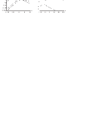
Fig. 1: (a) Energy spectra of a pure fractal line and (b), realistic vortex loop in superfluid turbulent HeII (see text).

In parallel to a ’counting of powers’ we performed a numerical calculation of the spectra with the help of Mathematica 3.0. In Fig.1a we depict (in logarithmic scale) three curves corresponding to the spectral density $E(k)$ for a pure fractal vortex filament of the length $L=100$ (all units are arbitrary). The upper curve (see the region of small $k$) corresponds to the case $\lambda=0$, i.e. to smooth lines. It can be seen how dependence $E(k)\propto k^{2}$ is changed to a dependence $E(k)\propto k^{-1}$ in the region of $k\sim 100^{-1}$. That is a general result, since $H_{D}=1$ and the $3D$ size of the curve is of order of $100$. The next (middle) curve corresponds to the case $\lambda=-4/5$, i.e. to the so called self-avoid line. It is seen again that a $k^{2}$-dependence is changed to a dependence $E(k)\propto k^{-1/3}$ in the region of $k\sim 100^{-3/5}$. Taking into account that $H_{D}=2/(\lambda+2)=5/3$, this behavior agrees with the general result. The lower curve corresponds to the pure random walk chain with $N(\xi_{1}-\xi_{2})=l_{0}\delta(\xi_{1}-\xi_{2}).$ Formally $\lambda=-1$, and $H_{D}=2.$ Therefore the $k^{2}$-dependance is changed to $k$-independent spectral density $E(k)\propto k^{0}$ in the region of $k\sim 100^{-1/2}$, as it should be.

Let us now consider a VT in HeII. As has been discussed earlier, the VT in HeII is a semi-fractal object, behaving as a smooth line for small separation $\Delta\xi\ll R$, and having a random walk structure for large $\Delta\xi$ with $H_{D}=2$ and with the effective step equal to $R$. Therefore the speculations based on ”counting of powers” are not applicable directly. However one can assert that the equipartition distribution of energy $E(k)\propto k^{2}$ in the region of $k<<1/\sqrt{LR}$ should take place for a vortex loop in turbulent HeII. The region of large wave numbers is divided with some additional value $k\sim 1/R$. One can suppose that at that point behavior of the spectrum changes, acquiring the properties of pure fractal with the corresponding HD in the according regions. Namely, $E(k)$ should scale as $k^{0}$ in region $1/R<<k$, and be approximately $k$-independent $1/\sqrt{LR}<<k<<1/R$ (provided the latter is broad enough). Numerical calculations confirm this conjecture. In Fig. 1b there is depicted (in logarithmic scale) the curves corresponding to the spectral density $E(k)$ for a vortex loop of length $L=100$ with $R=0.01$ and $R=1$. It is clearly seen that the upper curve ($R=0.01$ ) has three regions with bends at the points $k_{l}=1/\sqrt{LR}=1$, and $k_{r}=1/R=100.$ In three different parts we have $E(k)\propto k^{2}$, $E(k)\propto k^{0}$ and $E(k)\propto k^{-1}$, correspondingly. That is in excellent agreement with qualitative considerations. When the mean radius of curvature is equal $R=10,$ the correspondent $k_{l}=1/\sqrt{LR}\approx 0.03$, and $k_{r}=1/R=0.1$. This behavior agrees with recent numerical simulations$\sevenrm^{\hbox{\immediate{\bf?}}}$and our own.

4 Conclusion

Using the Gaussian approach for the chaotic vortex filament we calculate the energy spectrum $E(k)$ of the 3D random velocity field, induced by that VT. If the VT is assumed to be a purely fractal object, the $E(k)$ is a power-law function $E(k)\propto k^{-2+H_{D}}$. The spectrum of a more realistic VT also agrees with that formula, if one thinks of VT as a semi-fractal object with a varying (depending on scale) HD. Let us note that the HD of a simple noncorrelated vortex loops satisfies the condition $1<H_{D}<3$. That implies that Gaussian lines cannot create $3D$ flow, which has the Kolmogorov spectrum $E(k)\propto k^{-5/3}$. That implies that vortex loops should be strongly correlated (which, in turn, implies that the local approximation used in numerical calculations is invalid). Another variant is that the vortex filaments probably play no special role in turbulent flow.

References

- [1] U. Frisch, Turbulence (Cambridge University Press, Cambridge 1996)
- [2] K.W.Schwarz, Phys. Rev. B38, 2398 (1988)
- [3] S.K.Nemirovskii and W.Fiszdon, Rev. Mod. Phys., 67 , 37 (1995)
- [4] Makoto Tsubota, Tsunehiko Araki and Sergey K. Nemirovskii, Phys Rev. B62, 11751 (2000)
- [5] S.K. Nemirovskii, Phys. Rev B57, 5792 (1997)
- [6] M. Doi and S.F. Edwards, The theory of polymer dynamics (Clarendon Press, Oxford 1986)
- [7] D.Kivotides, J.Vassilicos, D.C. Samuels and C.F. Barenghi, Phys. Rev. Lett., 86, 3080 (2001)