Abstract

We compare two recently proposed methods for the characterization of phase transitions in small systems. The validity and usefulness of these approaches are studied for the case of the $q=4$ and $q=5$ Potts model, i.e. systems where a thermodynamic limit and exact results exist. Guided by this analysis we discuss then the helix-coil transition in polyalanine, an example of structural transitions in biological molecules.

Keywords: phase transitions, critical exponents, partition function zeros, Potts model, helix-coil transition.

PACS-No.: 05.70.Fh, 05.50.+q, 64.60.-i, 87.15.He

1 INTRODUCTION

The study of phase changes in macroscopic systems has a long tradition in statistical physics. Its basic assumption is that the dimensions of the macroscopic system are very large when compared with that of the constituting elements: phase transitions are well-defined only for infinite systems. However, there are many phenomena in finite systems which resemble phase transitions, see, for instance, Refs. [1, 2, 3, 4]. Because of their importance for the understanding of the physics of clusters of atoms [5] or the folding of proteins and other biological molecules [6], to name only a few examples, these “phase transitions” in small systems have recently attracted renewed interest. The main question is how the observed effects in small systems can be related to true phase transitions in macroscopic (or infinite) systems. A few attempts were recently made in this direction, either through studying for finite and small systems the topology of curvatures of the entropy-density surface $s(e,n)$ [7] in the microcanonical ensemble, or by exploring the density of complex zeros of their canonical partition function [4, 8].

The later approach is closer to the traditional view on phase transitions. For infinite systems the physical features of a phase transition can be obtained from the distribution of the complex zeros of partition functions of finite systems. As the number of complex zeros $\beta_{j}=\beta_{j}(L)$ grows with system size $L$ they will (for a system with no external field) pinch the positive real $\beta$-axis, and for large $L$ the corresponding value is the inverse of the physical critical temperature $T_{c}$. One example for the extension of these ideas to finite systems is the classification scheme by Borrmann et al. [4] which explores the linear behavior for the limiting density of zeros [9, 10]. Another description was suggested by Janke and Kenna (JK) who propose a new scaling relation to identify the order and strength of a transition from the behavior of small systems [8].

In this paper we try to evaluate the usefulness and validity of these two approaches. For this purpose we apply them to systems where a thermodynamic limit exists. In order to be useful the two approaches should be able to identify the macroscopic phase transition from investigations of small system sizes. Our test case is the 2D Potts model with $q=5$ states where the order of the phase transition is difficult to distinguish and which is therefore a challenging test for the new approaches. Simulations of the Potts model with $q=4$ states add data for the case of a second order phase transition. Our numerical investigations complement earlier work in Ref. [8] on the $q=10$ Potts model which has a pronounced first order phase transition.

Guided by our results for the Potts model we finally consider the helix-coil transition in polyalanine. The purpose of this investigation is to test whether the two approaches allow a characterization of structural transition in biological molecules.

2 PARTITION FUNCTION AND DENSITY OF COMPLEX ZEROS

In the canonical ensemble a system is completely described by its partition function

$$Z(\beta)=\sum_{E}n(E){\rm exp}(-\beta E)\,.$$ (1)

Introducing variables $u=\exp(-k\beta)$ with conveniently defined constant $k$ allows to write the partition function for discrete energy models as a polynominal:

$$Z(u)=\sum_{E}n(E)u^{E}~{}.$$ (2)

The number of complex zeros $u_{j}$, ($u_{j}={\rm exp}(-k\beta_{j}),j=1,2,...$) of this polynominal will grow with system size. In the case of a phase transition, we expect the zeros (or at least the ones close to the real axis) condense for large enough system size $L$ on a single line

$$u_{j}=u_{c}+r_{j}\,{\rm exp}(i\varphi)~{}.$$ (3)

As the system size $L$ increases, those zeros will move towards the positive real $u$-axis and the corresponding value is for large $L$ the inverse of the physical critical temperature $T_{c}$. Crucial information on phase transitions can be obtained from the way in which the first zero approaches the real $\beta$-axis. However, such an analysis depends on the extrapolation towards the infinite large system and does not allow characterization of the situation in small systems.

One possible extension of the above ideas to “phase transitions” in small systems is the classification scheme by Borrmann et al. [4]. The idea behind this scheme is to use not only the first complex zero $u_{1}$, but also higher zeros $u_{2},u_{3}$ and $u_{4}$. Writing the complex zeros as $u_{k}={\rm Re}(u_{k})+i\,\tau_{k}$, where $\tau_{k}$ stands for ${\rm Im}(u_{k})$, the assumed distribution of zeros on a straight line allows to define two parameters $\alpha_{u}$ and $\gamma_{u}$:

$$\alpha_{u}=\frac{{\rm ln}\,\phi(\tau_{3})-{\rm ln}\,\phi(\tau_{2})}{{\rm ln}\,\tau_{3}-{\rm ln}\,\tau_{2}}\,,\quad{\rm where}\quad\phi(\tau_{k})=\frac{1}{2}\left(\frac{1}{|{u}_{k}-{u}_{k-1}|}+\frac{1}{|{u}_{k+1}-{u}_{k}|}\right)\,,$$ (4)

with $k$ labelling the first zeros, and

$$\gamma_{u}=({\rm Re}(u_{2})-{\rm Re}(u_{1}))/(\tau_{2}-\tau_{1})\,.$$ (5)

Note, that our notation differs from that in Ref. [4] in that we define the discrete line density $\phi$ in function of the $u$-zeros instead of the temperature $\beta$. Following the classification scheme by Grossmann and Rosenhauer [9, 10], phase transitions can now be classified according to the values of these two parameters: for $\alpha_{u}\leq 0$ and $\gamma_{u}=0$ one has a phase transition of first order, it is of second order if $0<\alpha_{u}<1$ and arbitrary $\gamma_{u}$, and for $\alpha_{u}>1$ and arbitrary $\gamma_{u}$ one has a higher order transition. Besides the above parameters, $\tau_{1}$ plays also an important role: only for $\tau_{1}\rightarrow 0$ one obtains in the thermodynamic limit a real temperature for a phase transition.

Another extension of partition function zero analysis to small systems is the approach by Janke and Kenna (JK) [8] which uses that the average cumulative density of zeros [8]

$$G_{L}(r_{j})=\frac{2j-1}{2L^{d}}$$ (6)

can be written in the thermodynamic limit and for a first order transition as

$$G_{\infty}(r)=g_{\infty}(0)r+ar^{w+1}+\cdots\,.$$ (7)

Here, the slope at the origin is related to the latent heat, $\Delta e\propto g_{\infty}(0)$. Equations (3) and (7) imply that the distance $r_{j}$ of a zero from its critical point can be written for large enough lattice sizes as ${\rm Im}\,u_{j}(L)$ since ${\rm Re}\,u_{j}(L)\sim u_{c}$. Hence, in this limit Eq. (6) and (7) lead to the following scaling relation for the cumulative density of zeros as an equation in $j$ and $L$,

$$\frac{2j-1}{2L^{d}}=a_{1}({\rm Im}\,u_{j}(L))^{a_{2}}+a_{3}\,.$$ (8)

A necessary condition for the existence of a phase transition is that $a_{3}$ is compatible with zero, else it would indicate that the system is in a well-defined phase. The values of the constants $a_{1}$ and $a_{2}$ then characterize the phase transition. For instance, for first order transitions should the constant $a_{2}$ take values $a_{2}\sim 1$ for small $r$, and in this case the slope of this equation is related to the latent heat through the relation [8]

$$\Delta e=k\,u_{c}\,2\pi a_{1}\,,$$ (9)

with $u_{c}={\rm exp}(-k\beta_{c})$. On the other hand, a value of $a_{2}$ larger than $1$ indicates a second order transition whose specific heat exponent is given by $\alpha=2-a_{2}$.

The above approach was originally developed and tested for systems with well defined first order phase transitions such as the 2D 10-state Potts and 3D 3-state Potts model. The obtained results agree with previous work from numerical simulations and partition function zeros analysis of systems up to $L=64$ [11, 12] ($L=36$ for the 3D case [13]).

The classification of phase transitions by Borrmann et al. has been tested for the finite Bose-Einstein condensates in a harmonic trap and for small magnetic clusters and nuclear multifragmentation [4].

In the following we will show that despite these successful tests both approaches can lead to wrong conclusions if applied blindly. For this purpose we study systems where determination of the order of the phase transition is known to be computational difficult. We will concentrate on the 2D Potts model with $q=4$ (second order transition) and $q=5$ (weak first order transition) states since a series of exact results [14] exist for both models. For instance, the critical temperatures are known to be $\beta_{c}={\rm ln}(1+\sqrt{q})$ and the latent heat is given by $\Delta e(q=5)=0.0529187$. Finally, we research whether the two approaches can be used to characterize structural transitions in biological molecules.

3 RESULTS FROM POTTS MODEL SIMULATIONS

We start by presenting our results for the two Potts models with $q=4$ and $q=5$ on small lattices. Our study was performed on lattice sizes $L=16,32,64$ and $128$ for $q=4$ and $L=8,12,16,20,24,32,64,96\,$ and $128$ for $q=5$. For these models and system sizes we have evaluated the complex partition function zeros from heat-bath simulations with large statistics at temperatures $\beta_{0}$ listed in Table 1. For each lattice size, our results rely on 16 bins of 500000 measurements. For $L<96$ each measurement was separated by an additional Monte Carlo sweep which was discarded; for larger sizes measurements were only taken every 5th sweep.

For lattice sizes up to $L=20$, we could calculate all complex zeros from the polynominal form of the partition function using MATHEMATICA. For larger lattice sizes such a direct evaluation is no longer possible with standard numerical algorithms, even when double precision was used. Only by using the scan method (see [15] and references therein) we were able to obtain reliable estimates for the first $J$ complex zeros. Note, that $J$ is limited by the precision of our data: insufficient statistics of our simulation will lead to presence of so-called fake zeros [16]. For instance, for the $q=4$ Potts model we could only get reliable estimates for the first three zeros (Table 2) while for the $q=5$ Potts model we were able to obtain estimates for the first four partition function zeros (presented in Table 3). The error bars were calculated from the fluctuation of the averages taken over each of those 16 bins.

A The Borrmann Approach

From the listed zeros in Tables 2 and 3 we obtain our first result: even for our smallest lattice size ($L=16$ for $q=4$ and $L=8$ for $q=5$) the zeros stay on a straight line and the real parts are approximately constants. This is a necessary condition for both the Borrmann and the JK approach. We first calculate for both $q=4$ and $q=5$ Potts model the parameters $\alpha_{u}$ and $\gamma_{u}$ on which the Borrmann classification scheme relies. Their values are listed in Table 4 for all lattice sizes, and also plotted in Fig. 1a for the $q=4$ Potts model and in Fig. 1b for the case of $q=5$. For the $q=4$ Potts model we were only able to obtain reliable estimates for the first three zeros for each lattice size. However, in order to calculate the parameter $\alpha_{u}$ we need four zeros. For this reason, we have included here the less reliable fourth zero which is not listed in Table 2. As a consequence, our results for the $q=4$ Potts model are less reliable than these for the $q=5$ model where we have also acceptable estimates for the fourth zeros. Estimates and standard deviations presented in Table 4 were obtained by means of the bootstrap method [17] based on our statistics of 16 independent bins for each lattice size. Details on this method are presented in Appendix A.

For both models, the obtained values of Borrmann parameters $\alpha_{u}$ and $\gamma_{u}$ show no size dependence, but rather seems to fluctuate around some average value. For the case $q=4$, the values of $\alpha_{u}$ and $\gamma_{u}$ are compatible with the well-known fact that this model has a second order phase transition in the thermodynamic limit. However, our approach seems to fail for the case $q=5$ which has a weak first order phase transition and where we would expect $\alpha_{u}\leq 0$ and $\gamma_{u}=0$. Our results rather indicate a second order transition ($0<\alpha_{u}<1$ and $\gamma_{u}$ arbitrary). However, the $q=5$ Potts model is well-known to have a very large correlation length (of order 2000 lattice units [18]), and hence, its true behavior may only be caught for very large lattice sizes. Fig. 1b does not give any indications that we are even close to lattice sizes where the approach by Borrmann would lead to the correct result since the values for $\alpha_{u}$ and $\gamma_{u}$ show no systematic size dependence for the lattice sizes which we have studied ($L\leq 128$).

Our results indicate that an uncritical application of Borrmann approach may lead to wrong conclusions on the nature of phase transition in a system. In the case of the $q=5$ Potts model this approach fails to identify the nature of a phase transition from the distribution of zeros on small lattices. This seems to limit the usefulness of this method to systems where the order of the transition is clear.

B The JK Approach

A similar method to study phase transitions in small systems is the one proposed by Janke and Kenna [8]. In this approach one has to calculate the average cumulative density of zeros $G(r)$ from the zeros listed in Table 2 and 3. In order to investigate the phase transitions in our two systems one has to fit the cumulative density $G(r)$ to

$$G(r)=a_{1}r^{a_{2}}+a_{3}\,.$$ (10)

The aim of this fit is to obtain an estimate for $a_{3}$ since $a_{3}=0$ indicates the existence of a phase transition. However, a simple evaluation of this fit may be misleading if lattice sizes are too small. In this case it may be necessary to study the FSS dependence of these quantities, i.e. how their estimates are related to ones obtained for larger systems or even in the thermodynamic limit.

In the case of the $q=4$ Potts model we have to rely only on the first three zeros for each lattice size which is a too small number for a meaningful three-parameter fit. For this reason, we have combined the zeros of two neighboring lattice sizes and our fit therefore relies on six zeros for each pair. The so obtained estimates for $a_{3}(L)$ are listed in Table 5. For the case of the $q=5$ Potts model we have four zeros for each lattice size, but we have also calculated $a_{3}(L)$ from fits where the eight zeros of two neighboring lattice sizes were combined, which leads to a more robust estimate of this parameter. The so obtained sets of $a_{3}(L)$ are listed in Table 6. We note that for both models the values of $a_{3}(L)$ are for all lattice sizes compatible with zero, demonstrating that the two Potts models have indeed a phase transition.

The next question is whether and for what sizes the above approach is able to identify the order of the transition. This requires to calculate an accurate estimate for the quantity $a_{2}$ in Eq. (10). For this purpose, we set $a_{3}$ in Eq. (10) to zero and replace that equation by the simpler two-parameter fit

$$G(r)=a_{1}r^{a_{2}}~{}.$$ (11)

Extracting the parameters $a_{1}$ and $a_{2}$ from this fit requires an extremely careful data analysis and error estimation. For this reason we have again used the bootstrap method for estimating averages and standard errors. The obtained values of $a_{1}$ and $a_{2}$ are presented for all lattice sizes and both $q=4$ and $q=5$ in Tables 5 and 6. In Table 6 we list these parameters as a function of the first four complex zeros.

Let us first consider the case $q=4$. Fig. 2 displays the values for $a_{2}(L)$ as a function of lattice size. In this plot we do not observe any dependency of $a_{2}$ from the system size and the possibility of a first order transition ($a_{2}=1$) is clearly excluded. Hence, our analysis reproduces the well-known fact that the $q=4$ Potts model has a second order phase transition. However, with our estimate of $a_{2}$ from our largest lattice size, we find as critical exponent $\alpha=2-a_{2}=0.430(18)$. This value is far from the thermodynamic limit $2/3$ [19, 20, 21]. This discrepancy may be due to the dependence of $a_{2}(L)$ on the higher and less precise zeros in the fits. This dependence is less pronounced if we merge the zeros of all lattice sizes. Evaluating the resulting cumulative density leads to a value of $a_{2}=1.466(23)$ which corresponds to $\alpha=0.534(23)$. This value of the critical exponent $\alpha$ is closer to, but still far from the theoretical value. It follows that on the simulated lattice sizes the JK scaling relations do allow a qualitative characterization of the transition in the $q=4$ Potts model, but not to obtain quantitative results such as the numerical value of critical exponents. This limitation is a somehow surprising result since the density and the cumulative density of zeros seem to be free [8] from the multiplicative logarithmic corrections to the leading power-law finite-size behavior [21, 22] which hamper the determination of the critical exponents $\alpha$ and $\nu$ in other approaches.

At first sight, the situation seems to be worse for the $q=5$ Potts model. Even if we discard the fourth zero, which has larger fluctuations, and repeat our analysis only for the more reliable first three ones, our data do not lead to the expected result $a_{2}\sim 1$. This can also be seen from Fig. 2 where we plot also for this model the parameter $a_{2}(L)$ as a function of lattice size $L$. However, unlike in the Borrmann analysis of the $q=5$ Potts model, our data show a clear trend towards the expected value for a first order phase transition ($a_{2}\sim 1$). Our data suggest, that through by an extrapolation towards large (ideally infinite) lattices the true value of $a_{2}$ can be determined with the JK approach even for the $q=5$ Potts model. This is consistent with the fact that the $q=5$ Potts model has a very large correlation length (of order 2000 lattice units), and hence, its true behavior can only be caught for very large lattice sizes. The log-log plot of $a_{2}(L)$ in Fig. 3 indicates that one should use a polynominal fit for the extrapolation towards the thermodynamic limit:

$$a_{2}(L)=a_{2}(\infty)+bL^{-c}\,.$$ (12)

In order to see how acceptable the expected limit $a_{2}=1$ is, we replace the above equation by a two-parameter fit ${\rm ln}\,(a_{2}(L)-1)={\rm ln}\,b-c\,{\rm ln}L$ (i.e. we set $a_{2}=1$). In this way, we obtain $b=0.717(16)$ and $c=0.1765(69)$, with the goodness of fit [23] $Q=0.72$ for four zeros and $b=0.7910(88),\,c=0.2050(40)$, with a smaller $Q=0.09$ for three zeros. The corresponding fit for the case of four zeros is shown in Fig. 4 and demonstrates that our data are indeed compatible with the expected value $a_{2}\sim 1$ for a first order phase transition. However, we still can obtain acceptable fits ($Q>0.7$) for the whole range of $0\leq a_{2}\leq 1.013$ (but note that values of $a_{2}<1$ are difficult to interprete in the JK theory, and rather indicate numerical instabilities) which shows the difficulty in determining the order of the phase transition for the $q=5$ Potts model. Only if we restrict our analysis to the first three zeros the goodness of fit shows a maximum for $a_{2}\approx 1$.

The JK approach allows us also to calculate the latent heat for the case of a first order phase transition by means of Eq. (9). However, that equation is valid only when $a_{2}(L)=1$. In the case of the $q=5$ Potts model we have $a_{2}(L)>1$ for all lattice sizes. Hence, we can not use Eq. (9) to calculate the latent heat from our values of $a_{1}(L)$. Instead we have replaced Eq. (11) by

$$G_{L}(r)=A_{1}(L)r~{},$$ (13)

i.e. $a_{2}(L)$ is substituted in Eq. (11) by $a_{2}(\infty)$, and have studied the finite size scaling of the new quantity $A_{1}(L)$ which has the same limiting value than $a_{1}(L)$. Values for $A_{1}$ are listed in Table 6. In order to calculate the latent heat of the $q=5$ Potts-model we evaluate firstly $a_{1}=A_{1}(\infty)$ from the finite-size-scaling fit

$$A_{1}(L)=A_{1}(\infty)+BL^{-C}~{},$$ (14)

which leads with a goodness-of-fit $Q=0.68$ to the values $a_{1}=0.0284(18),B=1.381(21)$ and $C=0.6187(80)$ when the first four zeros are used for each lattice size. Restricting the analysis to $A_{1}(L)$ calculated only from the first three zeros at each lattice size leads to $a_{1}=0.03085(78)$ (with a goodness of fit $Q=0.75$). Applying Eq. (9) we therefore find as latent heat $\Delta e=0.0551(35)$ ($\Delta e=0.0599(15)$ in case of three zeros) which is very close to the theoretical value $\Delta e(q=5)=0.0529\cdots$. This result is surprisingly good when compared with other numerical estimates. For instance, a recent study using lattices of up to $L=4000$ led to a latent heat value of $\Delta e=0.054$ [24].

Note that Eq. (14) corresponds to the finite size scaling behavior of the specific heat if we identify $C=(1-\alpha)/\nu$ since the latent heat scales with $C_{v}\,\Delta T_{c}(L)$, and at the critical temperature we have $\Delta T_{c}(L)\sim L^{-1/\nu}$ and

$$C_{v}^{\rm max}(L)=c_{1}+c_{2}L^{\alpha/\nu}\,.$$ (15)

This allows us to identify theoretically a second correction term in Eq. (14):

$$A_{1}(L)=A_{1}(\infty)+B_{1}L^{-(1-\alpha)/\nu}+B_{2}L^{-1/\nu}~{}.$$ (16)

A check shows that our value of $C=0.6187(80)$ is indeed close to $(1-\alpha)/\nu=0.627$ where the values of the called pseudocritical exponents $\alpha=0.63(5)$ and $\nu=0.59(3)$ were taken from finite estimates in Ref. [18].

We also see from Eq. (16) that for a strong first order phase transition (as for instance in the earlier studied $q=10$ Potts model [8]) where we have $\nu=1/d$ and $\alpha=1$, we do not have the first correction term in Eq. (16). This explains why even from small lattice sizes very good estimates of the latent heat ($\Delta e=0.698(2)$ which one has to compare with the exact value for the $q=10$ Potts model: $\Delta e(q=10)=0.6960494$ [14]) could be obtained for the $q=10$ Potts model in Ref. [8]. In fact, these estimates can be easily improved by including a second correction term, which goes as $L^{-2}$ for this model towards the new value $\Delta e=0.696(92)$. The large error is due to the fact that only the largest sizes $L=32,38,48\,{\rm and}\,64$, for which the first correction term can be discarded, were considered in our calculation. Here, our data relies on the values quoted in Ref. [11].

Our results indicate the JK scaling relations are more suitable than the Borrmann approach for studying phase transitions from the behavior of small systems. Unlike the Borrmann approach the order of the phase transition could be determined for both the $q=4$ and the $q=5$ Potts model. In the latter case (and for the $q=10$ Potts model which has also a first order phase transition) it was possible to calculate the latent heat with good accuracy. However, the approach failed to give the correct value for the critical exponent $\alpha$ in the case of the $q=4$ Potts model which has a second order transition.

4 Helix-coil transition in polyalanine

A common, ordered structure in proteins is the $\alpha$-helix and it is conjectured that formation of $\alpha$-helices is a key factor in the early stages of protein-folding [25]. It is long known that $\alpha$-helices undergo a sharp transition towards a random coil state when the temperature is increased. The characteristics of this so-called helix-coil transition have been studied extensively [26]. In previous work [27, 28, 29] evidence was presented that polyalanine exhibits a phase transition between the ordered helical state and the disordered random-coil state when interactions between all atoms in the molecule are taken into account. Here, we revisit polyalanine and investigate the helix-coil transition by means of the partition function analysis with the classification scheme of Borrmann and Janke/Kenna.

Our investigation of the helix-coil transition for polyalanine is based on a detailed, all-atom representation of that homopolymer. Since one can avoid the complications of electrostatic and hydrogen-bond interactions of side chains with the solvent for alanine (a nonpolar amino acid), explicit solvent molecules were neglected. The interaction between the atoms was described by a standard force field, ECEPP/2,[30] (as implemented in the KONF90 program [31]). Chains of up to $N=30$ monomers were considered, and our results rely on multicanonical simulations [32] of $N_{sw}$ Monte Carlo sweeps starting from a random initial conformation, i.e. without introducing any bias. We chose $N_{sw}$=400,000, 500,000, 1,000,000, and 3,000,000 sweeps for $N=10$, 15, 20, and 30, respectively. Measurements were taken every fourth Monte Carlo sweep. Additional 40,000 sweeps ($N=10$) to 500,000 sweeps ($N=30$) were needed for the weight factor calculations by the iterative procedure described first in Refs. [32]. In contrast to our first calculation of complex zeros presented in Ref. [28], where we divided the energy range into intervals of lengths 0.5 kcal/mol in order to make Eq. (2) a polynomial in the variable $u=e^{-\beta/2}$, we avoided any approximation scheme in the present work. This because the above approximation works very well for the first zero, but not for the next ones. Since we need high precision estimates also for the next zeros we applied again the scan method.

In Table 7 we present our first four partition function zeros for 7 bins, although the fourth one is less reliable due to the presence of fake zeros. It is hardly possible to divide our production data in larger number of bins due to the limited statistics of our runs. Using again the bootstrap method we first calculated out of the zeros for each bin the parameters $\alpha_{u}$ and $\gamma_{u}$ which characterize in the Borrmann approach phase transitions in small systems. As one can see in Table 8 the so obtained values for polyalanine are characterized by large error bars and show no clear trend with chain length. It seems that the median of the $\alpha_{u}$ values is $\alpha_{u}=0$ which would indicate a first order transition. However, our data have too large errors to draw such a conclusion on the nature of the helix-coil transition.

For this reason, we tried instead the JK scaling relations. Table 9 lists the parameter $a_{3}(N)$ of Eq. (8). Here, the average cumulative density of zeros is replaced by

$$G_{N}(r_{j})=\frac{2j-1}{2N}\,,$$ (17)

where we have translated the linear length $L$ as $N^{1/d}$  [28]. Therefore all finite size scaling relations can be written is terms of the number of monomers $N$.

The values $a_{3}$ are compatible with zero for chains of all length indicating that we have indeed a phase transition. In order to evaluate the kind of transition we also calculate the parameters $a_{1}(N)$ and $a_{2}(N)$ which we also summarize in Table 9. Similar to the case of the $q=5$ Potts-model, the parameter $a_{2}(N)$ decreases with system size. The log-log plot of this quantity as a function of chain length in Fig. 5 suggests again a scaling relation

$$a_{2}(N)=a_{2}+bN^{-c}\,.$$ (18)

A numerical fit of our data to this function leads to a value of $a_{2}=1.31(4)$ with $Q=0.95$. Using $\alpha=2-a_{2}$ we find $\alpha=0.70(4)$ which is barely compatible with our previous value of $\alpha=0.86(10)$ in Ref. [28], obtained from the maximum of specific heat. A fit of all four chain lengths can also not exclude a value $a_{2}=1$ since we can find acceptable fits with $Q>0.55$ in the range $0.92<a_{2}<1.44$. However, a close examination of Fig. 5 shows that the $N=30$ data point shows a considerable deviation from the trend suggested by the smaller chain length. Since the $N=30$ data are the least reliable, we also evaluated Eq. (18) omitting the $N=30$ chain. This leads to a value of $a_{2}=1.16(1)$ and a critical exponent $\alpha=0.84(1)$ which is now compatible with our previous result $\alpha=0.86(10)$.

Let us summarize our results for the helix-coil transition studies of polyalanine. The JK approach is able to reproduce for polyalanine results obtained in previous work [28], but does not lead here to an improvement over other finite size scaling techniques. Especially, the JK approach does not allow to establish the order of the helix-coil transition from simulation of small chains. Our results for the parameter $a_{2}$ seem to favor a second order transition, but are due to large errors and disputed by Ref. [29] were indications for a finite latent heat were found. In the present study we considered only a special kind of biological molecules, homopolymers of amino acids, where in principle the thermodynamic limit can be considered. This allows finite size scaling which was an essential tool for obtaining the correct results with the JK approach. However, in general such finite size scaling is not possible for biomolecules that have a distinct size and composition. In these cases we have to rely on Borrmann’s approach. However, in our example of polyalanine, Borrmann’s approach led to even less conclusive results since the error bars were large. Hence, it seems that both approaches are limited in their usefulness for the study of phase-transitions in biomolecules.

5 Conclusion

We have evaluated two recently proposed schemes for characterizing phase transitions in small systems. Simulating the $q=4$ and $q=5$ Potts model, where for the thermodynamic limit we can compare our data with exact results, we found that both Borrmann and JK approach work well when the order of the phase transition is not in question (such as in the case of the $q=4$ Potts model (second order) or the earlier studied first order transition in the $q=10$ Potts model). The situation is different for cases such as the $q=5$ Potts model where it is difficult to distinguish between a weak first order or a strong second order transition. A careful application of the JK approach led to the correct result of a weak first order transition for the $q=5$ Potts model while the Borrmann approach did not allow a correct identification of this transition with the lattice sizes studied by us. Our results from Potts model simulations indicate that both approaches have to be applied with great care if one wants to avoid wrong conclusions on the nature of phase transition in a system. This may limit their usefulness to systems where the order of the transition is clear and to systems which are not too small. Especially, a first application of both approaches to helix-coil transitions in polyalanine demonstrates the difficulties appearing when they are applied to the study of phase transitions in biomolecules.

6 Appendix: Bootstrap method

Bootstrap is a simulation method based on a given data sample, to produce statistical inferences like standard error and bias-corrected estimator for the mean sample [17]. The bootstrap algorithm consider that our data can be obtained from an unknown probability distribution $F$ by random sampling

$$F\rightarrow{\rm\bf X}=(x_{1},x_{2},\cdots,x_{n})\,.$$ (19)

Here the points $x_{i}$ refer to our $n=16$ bins for each lattice size in the Potts model or to $n=6$ bins for polyalanine. For each bin, the points $x_{i}$ contain the first four complex zeros.

Our statistics of interest are estimates for mean values $\hat{\theta}=\theta({\rm\bf X})$ for the parameters $\alpha$ and $\gamma$ in the Borrmann approach

$$\hat{\alpha}={\cal F}(\rm\bf X)\,$$ (20)

$$\hat{\gamma}={\cal G}(\rm\bf X)$$ (21)

and their respectives standard errors ${\rm se}(\hat{\alpha})$ and ${\rm se}(\hat{\gamma})$. Here $\cal F$ and $\cal G$ stand for the application of functions in Eqs. (4) and (5).

The bootstrap algorithm follows by considering our sample as an empirical distribution $\hat{F}$, where each data has the probability $1/n$. The way bootstrap assigns an accuracy to our parameters does not depend on any theoretical calculation but random samples of size $n$ drawn with replacement from $\hat{F}$, called a bootstrap sample,

$$\hat{F}\rightarrow{\rm\bf X^{*}}=(x_{1}^{*},x_{2}^{*},\cdots,x_{n}^{*})\,,$$ (22)

where each value $x_{i}^{*}$ equals any one of the $n$ values $x_{i}$.

Therefore for each bootstrap sample ${\rm\bf X^{*}}$ there is a bootstrap replication of $\hat{\theta}$ which we denote as $\hat{\theta}^{*}$. If we repeat this process, the sample standard deviation can be obtained from $B$ replications

$$\hat{se}_{B}=\{\sum_{b=1}^{B}[\hat{\theta}^{*}(b)-\hat{\theta}^{*}(\cdot)]^{2}/(B-1)\}^{1/2}\,,$$ (23)

where the bootstrap mean $\hat{\theta}^{*}(\cdot)=\sum_{b=1}^{B}\hat{\theta}^{*}(b)/B$. The limit of $\hat{se}_{B}$ as $B$ goes to infinity gives the ideal bootstrap estimate of $se(\hat{\theta})$.

The histogram in Fig. 6 represents our $\hat{\theta}^{*}$ distribution for the parameter $\alpha$ in our simulation of the $q=4$ Potts model for $L=128$ with $B=400$ replications. We obtain the bootstrap mean $\hat{\alpha}^{*}=0.46(17)$. On the other hand, if calculating simple averages from our 16 measurements leads to $\hat{\alpha}=0.41(18)$.

The bootstrap estimate of bias based on $B$ replications is given by

$$\hat{bias}_{B}=\hat{\theta}^{*}(\cdot)-\hat{\theta}\,.$$ (24)

Therefore, the bias-corrected estimator is $\bar{\theta}=\hat{\theta}-\hat{bias}$. It is also convenient to evaluate the ratio of estimated bias to standard deviation $\hat{bias}_{400}/\hat{se}_{400}$. A small number indicates an unneeded bias correction in face of the standard error. The called root mean square error of estimator $\hat{\theta}$ for $\theta$ can be defined to take into account both bias and standard deviation [17],

$$\sqrt{E_{F}[(\hat{\theta}-\theta)^{2}]}=\sqrt{se_{F}(\hat{\theta})^{2}+bias_{F}(\hat{\theta},\theta)^{2}}\\ \simeq se_{F}(\hat{\theta})\,[1+\frac{1}{2}(\frac{bias_{F}}{se_{F}})]\,.$$ (25)

If we take $\hat{bias}=\hat{bias}_{400}$, our final result is $\bar{\alpha}=0.36(18)$ for $q=4$ and $L=128$. In the tables we quote our final estimates $\bar{\theta}=\hat{\theta}-\hat{bias}$ and the above bias-corrected standard errors.

Acknowledgements
U.H.E. Hansmann gratefully acknowledges support by research grant of the National Science Foundation (CHE-9981874), and N.A. Alves support by CNPq (Brazil). Part of this article was written when U.H. was visiting the University of Central Florida. He thanks Brian Tonner, Alfons Schulte and the other faculty at the Department of Physics for the kind hospitality extended to him.

Figure Captions:

  Figure 1.

$\alpha_{u}(L)$ and $\gamma_{u}(L)$ estimates for $q=4$ Potts model data (a) and for $q=5$ Potts model data (b).

  Figure 2.

The parameter $a_{2}(L)$ as function of system size $L$ for the $q=4$ Potts model and the $q=5$ Potts model.

  Figure 3.

The parameter $a_{2}(L)$ as a function of system size $L$ for the $q=5$ Potts model in a log-log plot.

  Figure 4.

$a_{2}(L)-1(=a_{2}(\infty))$ as a function of system size $L$ in a log-log plot. The straight line through the data points is from our fit.

  Figure 5.

The parameter $a_{2}(N)$ for polyalanine molecules of length $N$ in a log-log plot.

  Figure 6.

Histogram of 400 bootstrap replications for the parameter $\alpha_{u}$ from four-state Potts model data.

Table Captions:

  Table 1.

Heat-bath simulations at $\beta_{0}$ for four and five-state Potts model in two dimensions.

  Table 2.

Complex partition function zeros $u_{j},\,(j=1,2~{}{\rm and}~{}3)$ for four-state Potts model.

  Table 3.

Complex partition function zeros $u_{j},\,(j=1,2,3~{}{\rm and}~{}4)$ for five-state Potts model.

  Table 4.

Bootstrap bias-corrected estimates and bias-corrected standard error for the parameters $\alpha_{u}$ and $\gamma_{u}$ for $q=4$ and $q=5$.

  Table 5.

Bootstrap bias-corrected estimates and bias-corrected standard error for the JK parameters from first three zeros for $q=4$.

  Table 6.

Bootstrap bias-corrected estimates and bias-corrected standard error for the JK parameters from first four zeros for $q=5$.

  Table 7.

Partition function zeros for polyalanine.

  Table 8.

Bootstrap bias-corrected estimates and bias-corrected standard error for the parameters $\alpha_{u}$ and $\gamma_{u}$ for polyalanine model.

  Table 9.

Bootstrap bias-corrected estimates and bias-corrected standard error for the JK parameters for polyalanine.

Table 1.: Heat-bath simulations at $\beta_{0}$ for four and five-state Potts model in two dimensions.

$~{}L$	$\beta_{0}(q=4)$	$\beta_{0}(q=5)$
8		1.1283
12		1.1489
16	1.084	1.1580
20		1.1626
24		1.1655
32	1.090	1.16866
64	1.096	1.17240
96		1.17332
128	1.09755	1.17373

Table 2.: Complex partition function zeros $u_{j},\,(j=1,2~{}{\rm and}~{}3)$ for four-state Potts model.

$~{}L$	Re$(u_{1})$	Im$(u_{1})$	Re$(u_{2})$	Im$(u_{2})$	Re$(u_{3})$	Im$(u_{3})$
16	0.339010(28)	0.016483(33)	0.335906(66)	0.032757(84)	0.33423(40)	0.04589(23)
32	0.335633(37)	0.006419(20)	0.334563(48)	0.012875(52)	0.33430(18)	0.01787(22)
64	0.334196(10)	0.002482(19)	0.334034(47)	0.005050(31)	0.33359(17)	0.006824(77)
128	0.333674(10)	0.0009474(78)	0.333542(12)	0.001952(10)	0.33333(07)	0.002618(28)

Table 3.: Complex partition function zeros $u_{j},\,(j=1,2,3~{}{\rm and}~{}4)$ for five-state Potts model.

$~{}L$	Re$(u_{1})$	Im$(u_{1})$	Re$(u_{2})$	Im$(u_{2})$	Re$(u_{3})$	Im$(u_{3})$	Re$(u_{4})$	Im$(u_{4})$
8	0.321522(26)	0.033184(19)	0.313723(58)	0.067481(33)	0.30728(22)	0.09619(18)	0.3013(11)	0.1223(11)
12	0.316268(26)	0.018168(14)	0.312678(29)	0.037897(29)	0.31030(15)	0.05411(13)	0.30850(87)	0.06935(54)
16	0.313834(25)	0.011808(10)	0.311797(34)	0.024957(25)	0.31040(13)	0.03614(11)	0.30859(82)	0.04550(54)
20	0.312511(15)	0.008441(14)	0.311073(14)	0.018037(18)	0.310277(77)	0.026062(97)	0.30994(57)	0.03288(29)
24	0.311688(20)	0.006394(11)	0.310639(20)	0.013791(20)	0.310037(80)	0.020166(78)	0.31008(32)	0.02560(27)
32	0.310760(18)	0.0041194(87)	0.310158(13)	0.008993(17)	0.309810(42)	0.013193(55)	0.30957(18)	0.01651(15)
64	0.3096252(58)	0.0014120(24)	0.3094365(61)	0.0031623(42)	0.309353(14)	0.004685(17)	0.309370(58)	0.005988(64)
96	0.3093404(43)	0.0007373(31)	0.3092477(54)	0.0016948(52)	0.3092213(93)	0.0025327(81)	0.309199(33)	0.003198(25)
128	0.3092206(71)	0.0004654(28)	0.3091614(67)	0.0010790(32)	0.309135(11)	0.0016104(54)	0.309161(27)	0.002079(13)

Table 4.: Bootstrap bias-corrected estimates and bias-corrected standard error for the parameters $\alpha_{u}$ and $\gamma_{u}$ for $q=4$ and $q=5$.

	$q=4$			$q=5$
$~{}L$	$\alpha_{u}$	$\gamma_{u}$		$\alpha_{u}$	$\gamma_{u}$
8				0.402(55)	-0.2267(20)
12				0.322(51)	-0.1819(16)
16	0.65(12)	-0.1897(43)		0.42(11)	-0.1552(24)
20				0.479(84)	-0.1503(19)
24				0.510(74)	-0.1414(23)
32	0.38(13)	-0.1650(84)		0.541(93)	-0.1233(25)
64	0.44(16)	-0.058(18)		0.433(65)	-0.1074(15)
96				0.458(73)	-0.0970(46)
128	0.36(18)	-0.125(15)		0.329(40)	-0.0990(58)

Table 5.: Bootstrap bias-corrected estimates and bias-corrected standard error for the JK parameters from first three zeros for $q=4$.

$~{}L$	$a_{1}$	$a_{2}$	$(L,L^{\prime})$	$a_{3}$
16	1.26(03)	1.574(07)	(16, 32)	-0.00008(93)
32	1.48(10)	1.579(16)	(32, 64)	-0.00003(24)
64	1.83(19)	1.591(19)	(64, 128)	-0.000006(59)
128	1.86(22)	1.570(18)

Table 6.: Bootstrap bias-corrected estimates and bias-corrected standard error for the JK parameters from first four zeros for $q=5$.

$~{}L$	$a_{1}$	$a_{2}$	$A_{1}$	$a_{3}$	$(L,L^{\prime})$	$a_{3}$
8	1.305(28)	1.4981(78)	0.4119(18)	-0.002(25)	( 8, 12)	-0.0003(60)
12	1.200(27)	1.4546(63)	0.3236(12)	-0.001(11)	(12, 16)	-0.0003(37)
16	1.170(40)	1.4370(81)	0.2759(14)	-0.0001(55)	(16, 20)	-0.0001(24)
20	1.161(36)	1.4290(67)	0.2451(10)	-0.0001(35)	(20, 24)	-0.0001(16)
24	1.087(30)	1.4096(60)	0.22134(77)	0.0001(23)	(24, 32)	0.00006(91)
32	1.045(30)	1.3949(57)	0.19069(62)	0.0001(13)	(32, 64)	0.00001(17)
64	0.863(41)	1.3475(82)	0.13353(76)	0.00002(31)	(64, 96)	0.000009(85)
96	0.734(31)	1.3175(62)	0.11049(42)	0.00001(14)	(96, 128)	0.000007(50)
128	0.666(29)	1.3002(66)	0.09687(35)	0.000006(74)

Table 7.: Partition function zeros for polyalanine.

$~{}N$	Re$(u_{1})$	Im$(u_{1})$	Re$(u_{2})$	Im$(u_{2})$	Re$(u_{3})$	Im $(u_{3})$	Re$(u_{4})$	Im$(u_{4})$
10	0.30530(12)	0.07720(14)	0.2823(13)	0.13820(61)	0.2459(72)	0.1851(63)	0.172(11)	0.2200(71)
15	0.356863(61)	0.053346(39)	0.34167(60)	0.10440(59)	0.3331(48)	0.1454(28)	0.3067(81)	0.1689(32)
20	0.374016(41)	0.042331(45)	0.36161(27)	0.08109(24)	0.3569(27)	0.1154(13)	0.3336(56)	0.1470(27)
30	0.378189(19)	0.027167(32)	0.37399(14)	0.05420(27)	0.3693(11)	0.0804(13)	0.35854(63)	0.1022(43)

Table 8.: Bootstrap bias-corrected estimates and bias-corrected standard error for the parameters $\alpha_{u}$ and $\gamma_{u}$ for polyalanine model.

$~{}N$	$\alpha_{u}$	$\gamma_{u}$
10	-0.36(17)	-0.365(17)
15	0.41(19)	-0.291(11)
20	0.06(14)	-0.3229(78)
30	0.19(14)	-0.1568(58)

Table 9.: Bootstrap bias-corrected estimates and bias-corrected standard error for the JK parameters for polyalanine.

$~{}N$	$a_{1}$	$a_{2}$	$a_{3}$
10	6.17(60)	1.862(46)	0.01(14)
15	4.37(19)	1.664(16)	0.014(69)
20	3.62(26)	1.558(24)	-0.014(98)
30	3.54(31)	1.473(30)	-0.007(61)

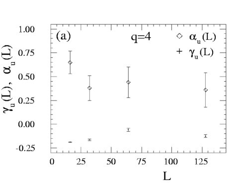
(Fig.1a) 1.: $\alpha_{u}(L)$ and $\gamma_{u}(L)$ estimates for $q=4$ Potts model data (a) and for $q=5$ Potts model data (b).

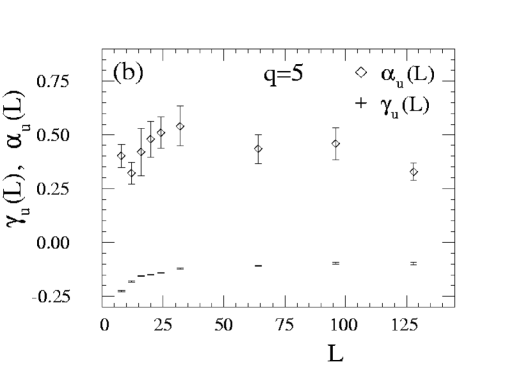
(Fig.1b) 2.:

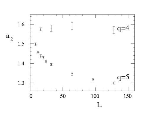
(Fig.2) 3.: The parameter $a_{2}(L)$ as function of system size $L$ for the $q=4$ Potts model and the $q=5$ Potts model.

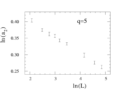
(Fig.3)  4.: The parameter $a_{2}(L)$ as a function of system size $L$ for the $q=5$ Potts model in a log-log plot.

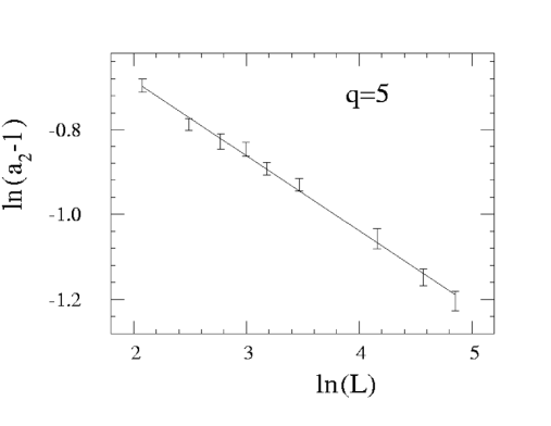
(Fig.4)  5.: $a_{2}(L)-1(=a_{2}(\infty))$ as a function of system size $L$ in a log-log plot. The straight line through the data points is from our fit.

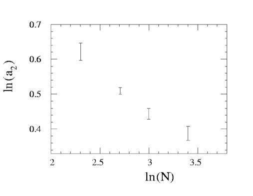
(Fig.5)  6.: The parameter $a_{2}(N)$ for polyalanine molecules of length $N$ in a log-log plot.

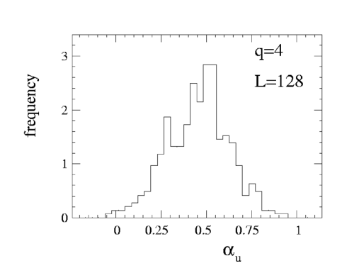
(Fig.6)  7.: Histogram of 400 bootstrap replications for the parameter $\alpha_{u}$ from four-state Potts model data.

REFERENCES

- [1] A. Chbihi, O. Schapiro, S. Salou and D.H.E. Gross, Eur. Phys. J. A5 (1999) 251
- [2] B. Borderie et al., Phys. Rev. Lett. 86 (2001)3252.
- [3] O. Lopez, Nucl. Phys. A685 (2001)246c.
- [4] P. Borrmann, O. Mülken and J. Harting, Phys. Rev. Lett. 84 (2000)3511; O. Mülken, P. Borrmann, J. Harting and H. Stamerjohanns, Phys. Rev. A64 (2001) 013611; O. Mülken and P. Borrmann, Phys. Rev. C63 (2001) 024306.
- [5] A. Proykova and R.S. Berry, Z. Phys. D. 40 (1997) 215.
- [6] C.B. Anfinsen, Science 181 (1973) 223.
- [7] D.H.E. Gross and E. Votyakov, Eur. Phys. J B15 (2000)115 ; D.H.E. Gross, Nucl. Phys. A681 (2001) 366c; D.H.E. Gross http://arXiv.org/abs/cond-mat/0006203; D.H.E. Gross http://arXiv.org/abs/cond-mat/0105313.
- [8] W. Janke and R. Kenna, J. Stat. Phys. 102 (2001) 1211; http://arXiv.org/abs/cond-mat/0103333.
- [9] S. Grossmann and W. Rosenhauer, Z. Physik 207 (1967)138.
- [10] S. Grossmann and W. Rosenhauer, Z. Physik 218 (1969)437; S. Grossmann and W. Rosenhauer, Z. Physik 218 (1969)449.
- [11] R. Villanova, Ph.D. Thesis (1991). Florida State University (unpublished).
- [12] R. Villanova, N.A. Alves and B.A. Berg, Nucl. Phys. B (Proc. Suppl.) 20 (1991) 665.
- [13] N.A. Alves, B.A. Berg and R. Villanova, Phys. Rev. B43 (1991) 5846.
- [14] F.Y. Wu, Rev. Mod. Phys. 54 (1982)235, erratum: Rev. Mod. Phys. 55 (1983)315.
- [15] N.A. Alves, J.R.D. de Felicio and U.H.E. Hansmann, Int. J. Mod. Phys. C8 (1997) 1063.
- [16] N.A. Alves, B.A. Berg and S. Sanielevici, Nucl. Phys. B376 (1992) 218.
- [17] B. Efron, SIAM Rev. 21 (1979) 460. B. Efron and R.J. Tibshirani,An introduction to the Bootstrap, Monographs on Statistics and Applied Probability 57 (Chapman & Hall, 1993).
- [18] P. Peczak and D.P. Landau, Phys. Rev. B39 (1989) 11932.
- [19] M. Nauenberg and D.J. Scalapino, Phys. Rev. Lett. 44 (1980) 837. J.L. Cardy, M. Nauenberg and D.J. Scalapino, Phys. Rev. B22 (1980) 2560.
- [20] R.J. Creswick and S-Y Kim, J. Phys.A: Math. Gen. 30 (1997) 8785.
- [21] J. Salas and A.D. Sokal, J. Stat. Phys. 88 (1997) 567.
- [22] M. Caselle, R. Tateo and S. Vinti, Nucl. Phys. B562 [FS] (1999) 549.
- [23] W. Press et al., Numerical Recipes (Cambridge University Press, London, 1986).
- [24] T. Nishino and K. Okunishi, J. Phys. Soc. Japan 67 (1998) 1492.
- [25] R.M. Ballew, J. Sabelko, and M. Gruebele, Proc. Nat. Acad. Sci. USA 93, 5759 (1996).
- [26] D. Poland and H.A. Scheraga, Theory of Helix-Coil Transitions in Biopolymers (Academic Press, New York, 1970).
- [27] U.H.E. Hansmann and Y. Okamoto, J. Chem. Phys. 110, 1267 (1999), 111 (1999) 1339(E).
- [28] N.A. Alves and U.H.E. Hansmann, Phys. Rev. Lett. 84 (2000) 1836.
- [29] J.P. Kemp, U.H.E. Hansmann and Zh.Y. Chen, Eur. Phy. J. B 15, 371 (2000).
- [30] M.J. Sippl, G. Némethy and H.A. Scheraga, J. Phys. Chem., 88, 6231 (1994); and references therein.
- [31] H. Kawai, Y. Okamoto, M. Fukugita, T. Nakazawa, and T. Kikuchi, Chem. Lett. 1991, 213 (1991); Y. Okamoto, M. Fukugita, T. Nakazawa, and H. Kawai, Protein Engineering 4, 639 (1991).
- [32] B.A. Berg and T. Neuhaus, Phys. Lett. 267, 249 (1991).